A Cool Load Balancer for Parallel Applications

(1)

A ‘Cool’ Load Balancer for Parallel Applications

Osman Sarood

Dept. of Computer Science University of Illinois at

Urbana-Champaign Urbana, IL 61801, USA

[email protected]

Laxmikant V. Kale

Dept. of Computer Science University of Illinois at

Urbana-Champaign Urbana, IL 61801, USA

[email protected]

ABSTRACT

Meeting power requirements of huge exascale machines of the future would be one major challenge. Our focus in this paper is to minimize cooling power and we propose a tech-nique, that uses a combination of DVFS and temperature aware load balancing to constrain core temperatures as well as save cooling energy. Our scheme is specifically designed to suit parallel applications which are typically tightly coupled. The temperature control comes at the cost of execution time and we try to minimize the timing penalty.

We experiment with three applications (with different power utilization profiles), run on a 128-core (32-node) cluster with a dedicated air conditioning unit. We calibrate the efficacy of our scheme based on three metrics: ability to control aver-age core temperatures thereby avoiding hot spot occurence, timing penalty minimization, and cooling energy savings. Our results show cooling energy savings of up to 57% with timing penalty mostly in the range of 2 to 20%.

1. INTRODUCTION

Cooling energy is a substantial part of the total energy spent by an High Performance Computing (HPC) computer room or a data center. According to some reports, this can be as high as 50% [19], [3], [17] of the total energy budget. It is deemed essential to keep the computer room adequately cold in order to prevent processor cores from overheating beyond their safe thresholds. For one thing, continuous operation at higher temperatures can permanently damage processor chips. Also, processor cores operating at higher temperatures consume more power while running identical computations at the same speeds due to the positive feed-back loop between temperature and power [8].

Cooling is therefore needed to dissipate the energy con-sumed by a processor chip, and thus to prevent overheating of the core. This consumed energy has a static and dynamic component. The dynamic component increases as the cube of the frequency at which the core is run. Therefore, an al-ternative way of preventing overheating is to reduce the

fre-Permission to make digital or hard copies of all or part of this work for personal or classroom use is granted without fee provided that copies are not made or distributed for profit or commercial advantage and that copies bear this notice and the full citation on the first page. To copy otherwise, to republish, to post on servers or to redistribute to lists, requires prior specific permission and/or a fee.

SC’11 Seattle, Washington USA

quency. Modern processors and operating systems support such frequency control (e.g. DVFS). With this, it becomes possible to run a computer in a room with high ambient temperature, by simply reducing frequencies whenever tem-perature goes above a threshold.

However, this method of temperature control is problem-atic for HPC applications, which tend to be tightly coupled. If only one of the cores is slowed down by 50%, the entire application will slow down by 50% due to dependencies be-tween computations on different processors. This is further exacerbated when the dependencies are global, such as when global reductions are used with a high-frequency. Since in-dividual processors may overheat at different rates, and at different points in time, and since physical aspects of the room and the air flow may create regions which tend to be hotter, the situation where only a small subset of processors are operating at a reduced frequency will be quite common. For HPC applications, this method therefore is not suitable as it is.

The question we address in this paper is whether we can substantially reduce cooling energy without a significant tim-ing penalty. Our approach involves a temperature-aware dynamic load balancing strategy. In some preliminary work presented at a workshop [16], we have shown the feasibility of the basic idea in the context of a single eight-core node. The contributions of this paper include development of a scalable load-balancing strategy demonstrated on 128 core machine, in a controlled machine room, and with explicit power measurements. Via experimental data, we show that cooling energy can be reduced to the extent of up to to 57%, with the timing penalty only in the range of 2 to 20% in most cases.

We begin in Section 2 by introducing the frequency con-trol method, and documenting the timing penalty it im-poses on HPC applications. In Section 3 we describe our temperature-aware load balancer. It leverages object-based overdecomposition and the load-balancing framework in the Charm++ runtime system. Section 4 outlines the experi-mental setup for our work. We then describe (Section 5) performance data to show that, with our strategy, the tem-peratures are retained within the requisite limits, while the timing penalties are small. Some interesting issues that arise in understanding how different applications react to temper-ature control are analyzed in Section 6. Section 7 undertakes a detailed analysis of the impact of our strategies on machine energy and cooling energy. Section 8 summarizes related work and sets our work in its context, which is followed by a summary in Section 9.

(2)

2. CONSTRAINING CORE TEMPERATURES

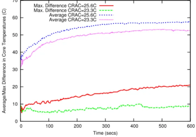
Unrestrained, core temperatures can soar very high. The most common way to deal with this in today’s HPC cen-ters is through the use of additional cooling arrangements. But as we have already mentioned, cooling itself accounts for around 50% [19, 3, 17] of the total energy consump-tion of a data center and this can rise even higher with the formation of hot spots. To motivate the technique of this paper, we start with a study of the interactions of core tem-peratures in parallel applications with the cooling settings of their surroundings. We runWave2D, a finite differenc-ing application, for ten minutes on 128 cores in our testbed. We provide more details of the testbed in Section 4. The cooling knob in this experiment was controlled by setting the cooling room air conditioning (CRAC) to different tem-perature settings. Figure 1 shows the average core temper-atures and the maximum difference of any core from the average temperature corresponding to two different CRAC set points. As expected, cooling settings have a pronounced effect on the core temperatures. For example, the average core temperatures corresponding to CRAC set point 23.3◦C are almost 6◦C less than those for CRAC set point 25.6◦C. Figure 1 also shows the maximum difference between the av-erage temperature and any core’s temperature and as can be seen, the difference worsens as we decrease external cooling (an increase of 11◦C). The result: Hotspots!

0 10 20 30 40 50 60 70 0 100 200 300 400 500 600

Average/Max Difference in Core Temperatures (C)

Time (secs) Max. Difference CRAC=25.6C Max. Difference CRAC=23.3C Average CRAC=25.6C Average CRAC=23.3C

Figure 1: Average core temperatures along with max. difference of any core from the average for Wave2D

The issue of core overheating is not new. DVFS is a widely accepted solution to cope with it. DVFS is a technique which is used to adjust the frequency and input voltage of a micro-processor. It is mainly used to conserve the dynamic power consumed by a processor. A shortcoming of DVFS, is that it comes with an execution time and machine energy penalty. To establish the severity of these penalties, we performed an experiment with 128 cores, runningWave2D for a fixed number of iterations. We used DVFS to keep core temper-atures under 44◦C by periodically checking core tempera-tures and reducing the frequency by one level whenever a core got hot. The experiment was repeated for five different CRAC set points. The results, in Figure 2 show the normal-ized execution time and machine energy. Normalization is done with respect to the run where all cores run at full fre-quency without DVFS. The high timing penalty (seen from Figure 2) coupled with an increase in machine energy makes

0 0.5 1 1.5 2 14.4 16.7 18.9 21.1 23.3 25.6

Normalized Execution Time/Energy

CRAC Set Point (C) Time Energy

Figure 2: Normalized time and machine energy us-ing DVFS forWave2D

it infeasible for HPC community to use such a technique. Now that we have established that DVFS on its own can not efficiently control core temperatures without incurring unacceptably high timing penalties, we now propose our ap-proach to ameliorate the deficiencies in using DVFS without load balancing.

3. TEMPERATURE AWARE LOAD

BALANC-ING

In this section, we propose a novel technique based on task migration that can efficiently control core temperatures and simultaneously minimizes the timing penalty. In addi-tion, it also ends up saving total energy. Although our tech-nique should work well with any parallel programming lan-guage which allows object migration, we chose Charm++ for our tests and implementation because it allows simple and straightforward task migration. We introduce Charm++ followed by a description of our temperature aware load bal-ancing technique.

3.1 Charm++

Charm++ is a parallel programming runtime system that works on the principle of processor virtualization. It vides a methodology where the programmer divides the pro-gram into small computations (objects or tasks) which are distributed amongst theP available processors by the run-time system [5]. Each of these small problems is a migrat-able C++ object that can reside on any processor. The runtime keeps track of the execution time for all these tasks and logs them in a database which is used by a load bal-ancer. The aim of load balancing is to ensure equal dis-tribution of computation and communication load amongst the processors. Charm++ uses the load balancing database to keep track of how much work each task is doing. Based on this information, the load balancer in the runtime sys-tem, determines if there is a load imbalance and if so, it migrates object from an overloaded processor to an under-loaded one [24]. The load balancing decision is based on the heuristic ofprinciple of persistance, according to which com-putation and communication loads tend to persist with time for a certain class of iterative applications. Charm++ load balancers have proved to be very successful with iterative applications such as NAMD [13].

(3)

3.2 Refinement based temperature aware load

balancing

We now describe our refinement based temperature aware load balancing scheme which does a combination of DVFS and intelligent load balancing of tasks according to frequen-cies in order to minimize execution time penalty. The gen-eral idea is to let each core work at the maximum possible frequency as long as it is within the maximum temperature threshold. Currently, we do DVFS on a per-chip instead of a per-core basis as the hardware did not allow us to do oth-erwise. When we change the frequency of all the cores on the chip, the core input voltage also drops resulting in power savings. This raises a question: What condition should trig-ger a change in frequency? In our earlier work [16], we did DVFS when any core on a chip crossed the temperature threshold. But our recent results show that basing DVFS decision on average temperature of the chip provides better temperature control. Another important decision is to de-termine how much should the frequency be lowered in case a chip exceeds the maximum threshold. Modern day pro-cessors come with a set of frequencies (frequency levels) at which they can operate. Our testbed had 10 different fre-quency levels from 1.2GHz to 2.4GHz (each step differs by 0.13GHz). In our scheme, we change the frequency by only one level at each decision time.

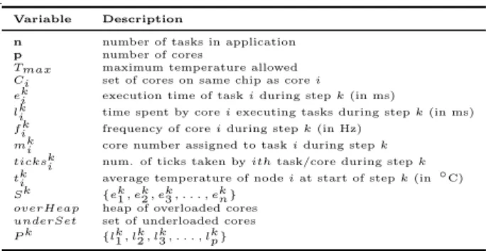
The pseudocode for our scheme is given in Algorithm 1 with the descriptions of variables and functions given in Ta-ble 1. The application specifies a maximum temperature threshold and a time interval at which the runtime periodi-cally checks the temperature and determines whether any node has crossed that threshold. The variable k in Al-gorithm 1 refers to the interval number the application is currently in. Our algorithm starts with each node comput-ing the average temperature for all cores present on it i.e. tk

i. Once the average temperature has been computed, each node matches it against the maximum temperature thresh-old (Tmax). If the average temperature is greater thanTmax, all cores on that chip shift one frequency level down. How-ever, if the average temperature is less than Tmax, we in-crease the frequency level of all the cores on that chip (lines 2-6). Once the frequencies have been changed, we need to take into account the speed differential with which each core can execute instructions. We start by gathering the load in-formation from the load balancing database for each core and task. In Charm++, this load information is maintained in milliseconds. Hence, in order to neutralize the frequency difference amongst the loads of each task and core, we con-vert the load times into clock ticks by multiplying load for each task and core with the frequency at which it was run-ning (lines 8-15). It is important to note that without doing this conversion, it would be incorrect to compare the loads and hence load balancing would result in inefficient sched-ules. Even with this conversion, the calculations would not be completely accurate, but will give much better estimates. We also compute the total number of ticks required for all the tasks (line 10) for calculating the weighted averages ac-cording to new core frequencies. Once the ticks are calcu-lated, we create amax heap i.e. overHeap, for overloaded and a set for underloaded cores i.e. underSet (line 16). The categorization of over and underloaded cores is done by theisHeavy and isLight procedures on lines (25-28). A coreiis overloaded if its currently assigned ticks are greater than what it should be assigned i.e. a weighted average of

Table 1: Description for variables used in Algorithm 1

Variable Description

n number of tasks in application

p number of cores

Tmax maximum temperature allowed

Ci set of cores on same chip as corei

ek_i execution time of taskiduring stepk(in ms)

lk_i time spent by coreiexecuting tasks during stepk(in ms)

f k_i frequency of coreiduring stepk(in Hz)

mk_i core number assigned to taskiduring stepk

ticksk_i num. of ticks taken byithtask/core during stepk

tk_i average temperature of nodeiat start of stepk(in◦C)

Sk {ek₁, ek₂, ek₃, . . . , ek_n}

overHeap heap of overloaded cores

underSet set of underloaded cores

P k {lk₁, lk₂, lk₃, . . . , lk_p}

totalT icks according to the cores new frequency (line 26). Notice the 1+tolerance factor in the expression at line 26. We have to use this in order to do refinement only for cores that are overloaded by some considerable margin. We set it to 0.03 for all our experiments. This means that a core is considered to be overloaded if its currently assigned ticks are greater than its average weighted ticks by a factor of 1.03. Similar check is in place forisLightprocedure (lines 27) but we do not include tolerance as it does not matter.

Once the max heap for the overloaded cores and a set for underloaded cores are ready, we start with the load balanc-ing. We pop the max element (tasks with maximum number of ticks) out ofoverHeap(referred asdonor). Next, we call the procedure getBestCoreAndTask which selects the best task to donate to the best underloaded core. The bestTask

is the largest task currently assigned todonor such that it does not overload a core from theunderSet. And the best-Core is the one which will remain underloaded after being assigned the bestTask. After determining thebestTask and

bestCore, we do the migration by recording the task mapping and (line 20) updating the donor andbestCore with num-ber of ticks in bestTask. We then callupdateHeapAndSet (line 23) which rechecks the donor for being overloaded. If it is, we reenter it tooverHeap. It also checks donor for be-ing underloaded so that it is added to theunderSet in case it has ended up with too little load. This ends the job of migrating one task from overloaded core to an underloaded core. We repeat this procedure untiloverHeapis empty. It is important to notice that the value of tolerance can affect the overhead of our load balancing. If that value is too large, it might ignore load imbalance whereas if it is too small, it can result in a lot of overhead for object migration. We have noticed that any value from 0.05 to 0.01 performs equally good.

4. EXPERIMENTAL SETUP

The primary objective of this work is to constrain core temperature and save energy spent on cooling. Our scheme ensures that all the cores fall below a user-defined maximum threshold. We want to emphasize that all results reported in this work are actual measurements and not simulations. We have used a 160 core (40 node, single socket) testbed equipped with a dedicated CRAC. Each node is a single socket machine with Intel Xeon X3430 chip. It is a quad core chip supporting 10 different frequency levels ranging from 1.2GHz to 2.4GHz. We use 128 cores out of the 160 cores available for all the runs that we report. All the nodes

(4)

Algorithm 1 Temperature Aware Refinement Load Bal-ancing

1: At nodeiat start of stepk 2: if tki > Tmaxthen 3: decreaseOneLevel(Ci) //reduce by 0.13GHz 4: else 5: increaseOneLevel(Ci) //increase by 0.13GHz 6: end if 7: At Master core 8: fori∈Sk−1do 9: tickski−1 =e k−1 i ×f k−1 mk_i−1

10: totalT icks=totalT icks+ticksk_i−1 11: end for 12: fori∈Pk−1 _do 13: ticksk_i−1=l_ik−1×f_ik−1 14: f reqSum=f reqSum+fik 15: end for 16: createOverHeapAndUnderSet() 17: whileoverHeapNOT NULLdo 18: donor =overHeap->deleteMaxHeap 19: (bestTask,bestCore) =

getbestCoreAndTask(donor,underSet) 20: mkbestT ask=bestCore

21: ticksk−1

donor=ticks k−1

donor−bestSize 22: ticksk_bestCore−1 =ticksk_bestCore−1 +bestSize

23: undateHeapAndSet()

24: end while

25: procedure isHeavy(i)

26: return (tickski−1 >(1 +tolerance) * (totalT icks*f k i) /f reqSum)

27: procedure isLight(i)

28: return (tickski−1 < totalT icks*f k

i/f reqSum)

run ubuntu 10.4 and we usecpufreqmodule in order to do DVFS. The nodes are interconnected using a 48-port gigabit ethernet switch. We use the Liebert Power unit installed with the rack to get power readings for the machines.

The CRAC in our testbed is an air cooler that uses cen-trally chilled water for cooling the air. It manipulates the flow of chilled water to achieve the temperature set point prescribed by the operator. The exhaust air (Thot) i.e. the hot air coming in from the machine room, is compared against the set point and the flow of the chilled water is adjusted ac-cordingly to cover the difference in the temperatures. This model of cooling is favorable considering that the tempera-ture control is responsive to the thermal load (as it tries to bring the exhaust air to temperature set point) instead of room inlet temperature [9]. The machines and the CRAC are located in the Computer Science department of Uni-versity of Illinois Urbana Champaign. We were fortunate enough to not only be able to use DVFS on all the available cores but to also change the CRAC set points.

There isn’t a straightforward way of measuring the exact power draw of the CRAC as it uses the chilled water to cool the air which in turn is cooled centrally for the whole build-ing. This made it impossible for us to use a power meter. But that isn’t unusual as most data centers use similar cool-ing designs. Instead of uscool-ing a power meter, we installed temperature sensors at the outlet and inlet of the CRAC. These sensors measure the air temperature coming from and going out to the machine room.

The heat dissipated into the air is affected by core temper-atures and the CRAC has to cool this air for maintaining a constant room temperature. The power consumed by CRAC (Pac) to bring the temperature of exhaust air (Thot) down to the cool inlet air (Tac) is [9]:

Pac=cair∗fac∗(Thot−Tac) (1) wherecair is the hear capacity constant,fac is the constant flow rate of the cooling system. Although we are not using a power meter, our results are very accurate because there is no interference from other heat sources as is the case with larger data centers where jobs from other users running on nearby nodes might dissipate a lot of heat which would dis-tort cooling energy estimation for your experiments.

To the best of our knowledge, this is the largest testbed on which any HPC researcher has reported results with DVFS. Also, we are not aware of any other work on constraining core temperatures and showing its benefit in cooling energy savings. In contrast to most of the earlier work that em-phasized on savings from machine power consumption using DVFS. Most importantly, our work is unique in using load balancing to mitigate effects of transient speed variations in HPC world.

We demonstrate the effectiveness of our scheme by us-ing three applications havus-ing different utilization and power profiles. The first is a canonical benchmark,Jacobi2D, that uses 5 point stencil to average values in a 2D grid using 2D decomposition. The second application,Wave2D, uses a finite differencing scheme to calculate pressure information over a discretized 2D grid. The third application, Mol3D, is from molecular dynamics and is a real world application to simulate large biomolecular systems. For Jacobi2D and

Wave2D, we choose a problem size of 22,000x22,000 and 30,000x30,000 grids respectively. For Mol3D however, we ran a system containing 92,224 atoms. We did an initial run of these applications without DVFS with CRAC working at 13.9◦C and noted the maximum average core ture reached for all 128 cores. We then used our tempera-ture aware load balancer to keep the core temperatempera-tures at 44◦C which was the maximum average temperature reached in the case ofJacobi2D (this was the lowest peak average temperature amongst all three applications). While keeping the threshold fixed at 44◦C, we decreased the cooling by increasing the CRAC set point. In order to gauge the effec-tiveness of our scheme, we compared it with the scheme in which DVFS is used to constrain core temperatures, without using any load balancing (we refer to it as w/o TempLDB

throughout the paper).

5. TEMPERATURE CONTOL AND TIMING

PENALTY

Temperature control is important for cooling energy con-siderations since it determines the heat dissipated into the air which the CRAC is responsible for removing. In addition to that, core temperatures and power consumption of a ma-chine are related with a positive feedback loop, so that an increase in any of them causes an increase in the other [8]. Our earlier work [16] shows evidence of this where we ran

Jacobi2D on a single node with 8 cores and measured the machine power consumption along with core temperatures. The results showed that increase in core temperature can cause an increase of up to 9% in machine power

(5)

consump-tion and this figure can be huge for large data centers. For our testbed in this work, Figure 3 shows the average temper-ature for all 128 cores over a period of 10 minutes using our temperature aware load balancing. The CRAC was set to 21.1◦C for these experiments. The horizontal line is drawn as a reference to show the maximum temperature threshold (44◦C) used by our load balancer. As we can see, irrespec-tive of how large the temperature gradient is, our scheme is able to restrain core temperature to within 1◦C. For ex-ample, core temperatures forMol3DandWave2Dreach the threshold i.e. 44◦C much sooner than Jacobi2D. But all three applications stay very close to 44◦C after reaching the threshold. 15 20 25 30 35 40 45 50 55 0 100 200 300 400 500 600 Average Temperature (C) Time (secs) Wave Jacobi Mol3D

Figure 3: Average core temperature with CRAC set point at21.1◦C 0 5 10 15 20 25 30 0 100 200 300 400 500 600

Max Difference in Core Temperature (C)

Time (secs) Without DVFS CRAC=25.6C Without DVFS CRAC=23.3C TempLDB Set Point=25.6C TempLDB Set Point=23.3C

Figure 4: Max difference in core temperatures for Wave2D

Temperature variation across nodes is another very im-portant factor. Spatial temperature variation is known to cause hot spots which can drastically increase the cooling costs of a data center. To get some insight into hot spot for-mation, we performed some experiments on our testbed with different CRAC set points. Each experiment was run for 10 minutes. Figure 4 shows the maximum difference any core has from the average core temperature for Wave2D when run with different CRAC set points. The Without DVFS

run refers to all cores working at full frequency and no tem-perature control at core-level. It was observed that for the

case ofWithout DVFS run, the maximum difference is due to one specific node getting hot and continuing to be so throughout the execution i.e. a hot spot. On the other hand, with our scheme, no single core is allowed to get a lot hotter than the maximum threshold. Currently, for all our experiments, we do temperature measurement and DVFS after every 6-8 seconds. More frequent DVFS would result in more execution time penalty since there is some overhead of doing task migration to balance the loads. We will return to these overheads later in this section.

The above experimental results showed the efficacy of our scheme in terms of limiting core temperatures. However, as shown in Section 2, this comes at the cost of execution time. We now use savings in execution time penalty as a metric to establish the superiority of our temperature aware load balancer in comparison to using DVFS without any load balancing. For this, we study the normalized execution times,tnorm, with and without our temperature aware load balancer, for all three applications under consideration. We definetnormas follows:

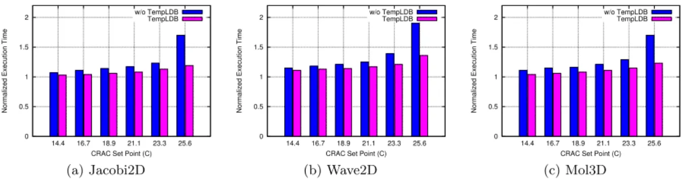
tnorm=tLB/tbase (2) where tLB represents the execution time for temperature aware load balanced run andtbaseis execution time without DVFS so that all cores work at maximum frequency. The value fortnormin case ofw/o TempLDBrun is calculated in a similar manner except that we usetN oLB instead oftLB. We experiment with different CRAC set points. All the ex-periments were performed by actually changing the CRAC set point and allowing the room temperature to stabilize be-fore any experimentation and measurements were done. To minimize errors, we averaged the execution times over three similar runs. Each run takes longer than 10 minutes to allow fair comparison between applications. The results of this ex-periment are summarized in Figure 5. The results show that our scheme consistently performs better thanw/o TempLDB

scheme as manifested by the smaller timing penalties for all CRAC set points. As we go on reducing the cooling (i.e. in-creasing the CRAC set point), we can see degradation in the execution times i.e. an increase in timing penalty. This is not unexpected and is a direct consequence of the fact that the cores heat up in lesser time and scale down to lower frequency thus taking longer to complete the same run.

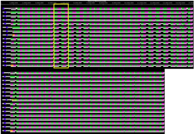
Figure 6: Projections timeline with and without Temperature Aware Load Balancing forWave2D

(6)

0 0.5 1 1.5 2 14.4 16.7 18.9 21.1 23.3 25.6

Normalized Execution Time

CRAC Set Point (C) w/o TempLDB TempLDB (a) Jacobi2D 0 0.5 1 1.5 2 14.4 16.7 18.9 21.1 23.3 25.6

CRAC Set Point (C) w/o TempLDB TempLDB (b) Wave2D 0 0.5 1 1.5 2 14.4 16.7 18.9 21.1 23.3 25.6

CRAC Set Point (C) w/o TempLDB

TempLDB

(c) Mol3D

Figure 5: Normalized execution time with and without Temperature Aware Load Balancing

Figure 7: Zoomed Projections for 2 iterations

It is interesting to observe from Figure 5 that the differ-ence in our scheme and thew/o TempLDB scheme is small to start with but grows as we increase the CRAC set point. This is because when the machine room is cooler, the cores take longer to heat up in the first place. As a result, even the cores falling in the hot spot area do not become so hot that they go to a very small frequency (we decrease fre-quency in steps of 0.13GHz). But as we keep on decreasing the cooling, the hot spots become more and more visible, so much so that when the CRAC set point is 25.6◦C, Node 10 (hot spot in our testbed) runs at the minimum possible frequency almost throughout the experiment. Our scheme does not suffer from this problem since it intelligently assigns loads by taking core frequencies into account. But without our load balancer, the execution time increases greatly (re-fer to Figure 5 for CRAC set point 25.6◦C). This happens because in the absence of load balancing, execution time is determined by the slowest core i.e. core with the minimum frequency. 1.4 1.6 1.8 2 2.2 2.4 2.6 0 100 200 300 400 500 600 Minimum Frequency (GHz) Time (secs) Wave2D Jacobi2D Mol3D

Figure 8: Minimum frequency for all three applica-tions

For a more detailed look at our scheme’s sequence of ac-tions, we use Projections [6], a performance analysis tool from the Charm++ infrastructure. Projections provides a visual demonstration of multiple performance data including processor timelines showing their utilization. We carried out an experiment on 16-cores instead of 128 and use projections to highlight the salient features of our scheme. We worked with a smaller number of cores since it would have been dif-ficult to visually understand a 128-core timeline. Figure 6 shows the timelines and corresponding utilization for all 16 cores throughout the execution of Wave2D. Both runs in the figure had DVFS enabled. The upper run i.e. the top 16 lines, is the one whereWave2Dis executed without temper-ature aware load balancing whereas the lower part i.e. the bottom 16 lines, repeated the same execution with our tem-perature aware load balancing. The length of the timeline indicates the total time taken by an experiment. The green and pink colors show the computations, whereas the white lines represents idle time. Notice that the execution time with temperature aware load balancing is much less than that without it. To see how processors spend their time, we zoomed into the boxed part of Figure 6 and reproduced it in Figure 7. It represents 2 iterations of Wave2D. This zoomed part belongs to the run without temperature aware load balancing. We can see that because of DVFS, the first four cores work at a lower frequency than the remaining 12 cores. They, therefore, take longer to complete their tasks as compared to the remaining 12 cores (longer pink and green portions on the first 4 cores). The remaining 12 cores finish their work quickly and then keep on waiting for the first 4 cores to complete their tasks (depicted by white spaces to-wards the end of each iteration). These results clearly sug-gest that the timing penalty is dictated by the slowest cores. We also substantiate this by providing Figure 8 which shows the minimum frequency of any core during aw/o TempLDB

run (CRAC set point at 23.3◦C). We can see from Figure 5 thatWave2D andMol3dhave higher penalties as compared toJacobi2D. This is because the minimum frequency reached in these applications is lower than that reached inJacobi2D. We now discuss the overhead associated with our temper-ature aware load balancing. As outlined in Algorithm 1, our scheme has to measure core temperatures, do DVFS, decide new assignments and then exchange tasks according to the new schedule. The major overhead in our scheme comes from the last item i.e. exchange of tasks. In compari-son, temperature measurements, DVFS, and load balancing decisions take negligible time. To calibrate the

(7)

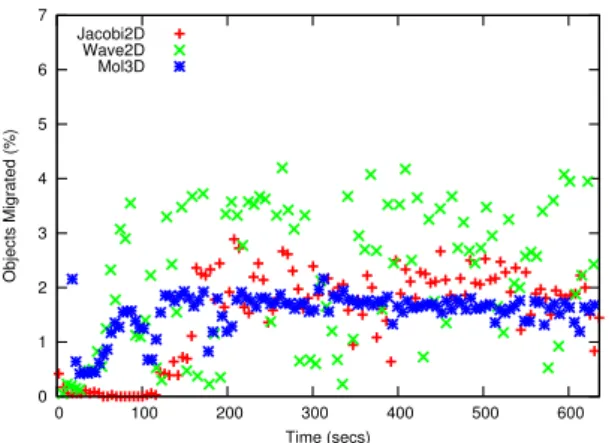
0 1 2 3 4 5 6 7 0 100 200 300 400 500 600 Objects Migrated (%) Time (secs) Jacobi2D Wave2D Mol3D

Figure 9: Percent objects migrated during temper-ature aware load balancer run

tion load we incur on the system, we run an experiment with each of the three applications for ten minutes and count the number of tasks migrated at each step when we check core temperatures. Figure 9 shows these percentages for all three applications. As we can see, the numbers are very small to make any significant difference. The small overhead of our scheme is also highlighted by its superiority over the w/o TempLDB scheme which does temperature control through DVFS but no load balancing (and so, no object migration). One important observation to be made from this figure is the larger number of migrations inWave2Das compared to the other two applications. This is because it has a higher CPU utilization. Wave2D also consumes/dissipates more power than the other two applications and hence has more transitions in its frequency. We explain and verify these application-specific differences in power consumption in the next Section.

6. UNDERSTANDING APPLICATION

REAC-TION TO TEMPERATURE CONTROL

One of the reasons we chose to work with three different applications was to be able to understand how application-specific characteristics react to temperature control. In this section, we highlight some of our findings and try to provide a comprehensive and logical explanation for them.

1.6 1.8 2 2.2 2.4 2.6 0 100 200 300 400 500 600 Average Frequency (GHz) Time (secs) Wave2D Jacobi2D Mol3D

Figure 10: Average frequency for all three applica-tions with CRAC at23.3◦C

We start by referring back to Figure 5 which shows that

Wave2Dsuffers the highest timing penalty followed byMol3D

and Jacobi2D. Our intuition was that this difference could be explained by the frequencies at which each application is running along with their CPU utilizations (see Table 2). Figure 10 shows the average frequency across all 128 cores during the execution time for each application. We were sur-prised with Figure 10 because it showed that bothWave2D

andMol3Drun at almost the same average frequency through-out the execution time and yet Wave2D ends up having a much higher penalty than Mol3D. Upon investigation, we found that Mol3D is less sensitive to frequency than

Wave2D. To further gauge the sensitivity of our applications to frequency, we ran a set of experiments in which each ap-plication was run at all available frequency levels. Figure 11 shows the results where execution times are normalized with respect to a base run where all 128 cores run at maximum frequency i.e. 2.4GHz. We can see from Figure 11 that

Wave2D has the steepest curve indicating its sensitivity to frequency. On the other hand, Mol3D is the least sensitive to frequency as shown by its small slope. This gave us one explanation for the higher timing penalties forWave2D as compared to the other two. However, if we use this line of reasoning only, then Jacobi2D is more sensitive to fre-quency (as shown by Figure 11) and has a higher utilization (Table 2) and should therefore have a higher timing penalty thanMol3D. But Figure 5 suggests otherwise. Moreover, the average power consumption ofJacobi2D is also higher than

Mol3D(see Table 2) which should imply cores getting hotter sooner while runningJacobi than withMol3d and shifting to lower frequency level. On the contrary, Figure 10 shows

Jacobi running with a much higher frequency thanMol3D. These counter intuitive results could only be explained in terms of CPU power consumption which is higher in case of

Mol3D than forJacobi2D. To summarize, these results sug-gest that although the total power consumption of the entire machine is smaller forMol3D, the proportion consumed by CPU is higher as compared to the same forJacobi2D.

For some mathematical backing to our claims, we look at the following expression for core temperatures [9]:

Tcpu=αTac+βPi+γ (3) HereTcpuis the core temperature,Tacis temperature of the air coming from the cooling unit,Piis power consumed by the chip, α, β and γ are constants which depend on heat capacity and air flow since our CRAC maintains a constant airflow. This expression shows that core temperatures are dependent on power consumption of the chip rather than the whole machine, and therefore it is possible that the cores get hotter forMol3D earlier than withJacobi2D due to higher CPU power consumption.

So far, we have provided some logical and mathemati-cal explanations for our counter-intuitive results. But we wanted to explore them thoroughly and find more cogent evidence to our claims. As a final step towards this ver-ification, we ran all three applications on 128 cores using the performance capabilities of Perfsuite [7] and collected information about different performance counters summa-rized in Table 2. We can see thatMol3D faces fewer cache misses and has 10 times more traffic between L1 and L2 cache (counter type ’Data Traffic L1-L2’) resulting in higher MFLOP/s thanJacobi2D. The difference between the total power consumption ofJacobi2D andMol3D can now be

(8)

ex-Table 2: Performance counters for one core

Counter Type Jacobi2D Mol3D Wave2D

Execution Time (secs) 474 473 469

MFLOP/s 240 252 292

Traffic L1-L2 (MB/s) 995 10,500 3,044

Traffic L2-DRAM (MB/s) 539 97 577

Cache misses to DRAM (billions) 4 0.72 4.22

CPU Utilization (%) 87 83 93

Power (W) 2472 2353 2558

Memory Footprint(% of memory) 8.1 2.4 8.0

plained in terms of more DRAM access forJacobi2D. We sum our analysis up by remarking that MFLOP/s seems to be the most viable deciding factor in determining the timing penalty that an application would have to bear when cool-ing in the machine room is lowered. Figure 12 substantiates our claim. It shows that Wave2D, which has the highest MFLOP/s (Table 2) suffers the most penalty followed by

Mol3D andJacobi2D.

1 1.2 1.4 1.6 1.8 2 2.2 1.4 1.6 1.8 2 2.2 2.4

Normalized Execution Time (C)

Frequency (GHz) Wave2D

Jacobi2D Mol3D

Figure 11: Normalized execution time for different frequency levels 0 5 10 15 20 25 30 35 40 14 16 18 20 22 24 26 Timing Penalty (%)

CRAC Set Point (C) Wave2D

Jacobi2D Mol2D

Figure 12: Timing penalty for different CRAC set points

7. ENERGY SAVINGS

This section is dedicated to a performance analysis for our temperature aware load balancing in terms of energy consumption. We first look at machine energy and cooling energy separately and then combine them to look at the total energy.

7.1 Machine Energy Consumption

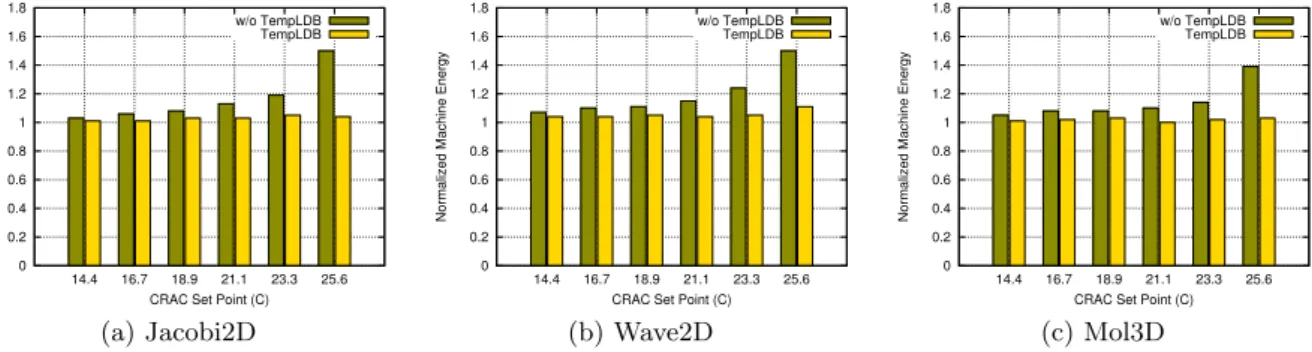
Figure 13 shows the normalized machine energy consump-tion (enorm), calculated as:

enorm=eLB/ebase (4)

whereeLB represents the energy consumed for temperature aware load balanced run andebase is execution time with-out DVFS with all cores working at maximum frequency. enorm, forw/o TempLDB run is calculated in a similar way with eLB replaced byeN oLB. Static power of CPU, along with the power consumed by power supply, memory, hard disk and the motherboard mainly form the idle power of a machine. A node of our testbed has an idle power of 40W which represents 40% of the total power when the machine is working at full frequency assuming 100% CPU utiliza-tion. It is this high idle/base power which inflates the total machine consumption in case of ‘w/o TempLDB’ runs as shown in Figure 13. This is because for every extra sec-ond of penalty in execution time, we will pay an extra 40J per node in addition to the dynamic energy consumed by the CPU. Considering this, our scheme does well to keep the normalized machine energy consumption close to 1 as shown in Figure 13.

We can better understand the reason why thew/o Tem-pLDB run is consuming much more power than our scheme if we refer back to Figure 7. We can see that although the lower 12 cores are idle after they are done with their tasks (white portion enclosed in the rectangle), they still consume idle power thereby increasing the total energy consumed.

7.2 Cooling Energy Consumption

While there exists some literature discussing techniques for saving cooling energy, those solutions are not applicable to HPC where applications are tightly coupled. Our aim in this work, is to come up with a framework for analyzing cooling energy consumption specifically from the perspective of HPC systems. Based on such a framework, we can de-sign mechanisms to save cooling energy that are particularly suited to HPC applications. We now refer to Equation 1 to infer thatThot andTac, are enough to compare energy con-sumption for CRAC as the rest are constants.

So we come up with the following expression for normal-ized cooling energy (cnorm):

cnorm= ThotLB−T LB ac Tbase hot −Tacbase ∗tLBnorm (5)

whereThotLBrepresents temperature of hot air leaving the ma-chine room (entering the CRAC) and TacLB represents tem-perature of the cold air entering the machine room respec-tively when using temperature aware load balancer. Sim-ilarly, when running all the cores at maximum frequency without any DVFS,Thotbaseis the temperature of hot air leav-ing the machine room andTbase

ac is the temperature of the cold air entering the machine room. tnormis the normalized time for the temperature aware load balanced run. Notice

(9)

0 0.2 0.4 0.6 0.8 1 1.2 1.4 1.6 1.8 14.4 16.7 18.9 21.1 23.3 25.6

Normalized Machine Energy

CRAC Set Point (C) w/o TempLDB TempLDB (a) Jacobi2D 0 0.2 0.4 0.6 0.8 1 1.2 1.4 1.6 1.8 14.4 16.7 18.9 21.1 23.3 25.6

CRAC Set Point (C) w/o TempLDB TempLDB (b) Wave2D 0 0.2 0.4 0.6 0.8 1 1.2 1.4 1.6 1.8 14.4 16.7 18.9 21.1 23.3 25.6

TempLDB

(c) Mol3D

Figure 13: Normalized machine energy consumption with and without Temperature Aware Load Balancing

that we include the timing penalty in our cooling energy model so that we incorporate the additional time for which cooling must be done.

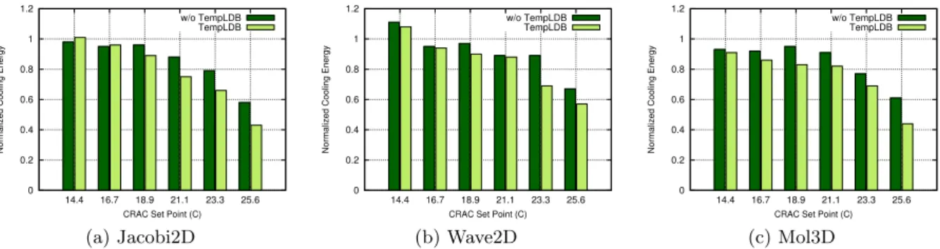
Figure 14 shows the normalized cooling energy for both with and without temperature aware load balancer. We can see from the figure that both schemes end up saving some cooling energy but temperature aware load balancing out-performs w/o TempLDB scheme by a significant margin. Our temperature readings showed that the difference be-tweenThot and Tac was very close in both cases i.e. our scheme and thew/o TempLDB scheme, and the savings in our scheme was a result of savings fromtnorm.

7.3 Total Energy Consumption

Although most data centers report cooling to account for 50% [19, 3, 17] of total energy, we decided to take a con-servative figure of 40% [11] for it in our calculations of total energy. Figure 15 shows the percentage of total energy we save and the corresponding timing penalty we end up pay-ing for it. Although it seems thatWave2D does not give us much room to decrease its timing penalty and energy, we would like to mention that our maximum threshold of 44◦C was very conservative for it. On the other hand, results from

Mol3DandJacobi2D are very encouraging in the sense that if a user is willing to sacrifice some execution time, he can save a considerable amount of energy keeping core temper-atures in check. It should also be noticed that our current constraints are very strict considering that we do not allow any core to go above the threshold. If we were to allow for a range of temperatures instead of one strict threshold, we can improve the timing penalty even more. For example, we did an experiment withMol3D, where the allowed core tem-perature range was set to 44◦C−49◦C and CRAC set point was 23.3◦C. With these settings, we saved 18% energy after paying only 4% timing penalty.

To quantify energy savings achievable with our technique, we plot normalized time against normalized energy (Fig-ure 16). The fig(Fig-ure shows data points for both our scheme andw/o TempLDB scheme. We can see that for each CRAC set point, our scheme moves the correspondingw/o Tem-pLDB point towards the left (reducing energy) and down (reducing timing penalty). The slope of these curves would give us the number of seconds the execution time increases for each joule saved in energy. As we see Jacobi2D has a higher potential for energy saving as compared to Mol3D

because of the lower MFLOP/s.

8. RELATED WORK

Most researchers from HPC have focused on minimiz-ing machine energy consumption as opposed to coolminimiz-ing en-ergy [15, 1, 21]. Given a target program, a DVFS enabled cluster, and constraints on power consumption, they [18] come up with a frequency schedule that minimizes execu-tion time while staying within the power constraints. Our work differs in that we base our DVFS decisions on core tem-peratures for saving cooling energy whereas they devise fre-quency schedules according to task schedule irrespective of core temperatures. Their scheme works with load balanced applications only whereas ours has no such constraints. In fact one of the major features of our scheme is that it strives to achieve a good load balance. A runtime system named, PET (Performance, power, energy and temperature manage-ment), by Hanson et al [4], tries to maximize performance while respecting power, energy and temperature constraints. Our goal is similar to them but we achieve it in a multicore environment which adds an additional dimension of load bal-ancing.

The work of Banarjee et al [1] comes closest to ours in the sense that they also try to minimize cooling costs in an HPC data center. But their focus is on controlling the CRAC set points rather than the core temperatures. In addition, they need to know the job start and end times beforehand to come up with the correct schedule whereas our technique does not rely on any pre-runs. Merkel et al [10] also explore the idea of task migration from hot to cold cores. However, they do not do it for parallel applications and therefore do not have to deal with complications in task migration decisions be-cause of synchronization primitives. In another work, Tang et al.[21] have proposed a way to decrease cooling and avoid hot spots by minimizing the peak inlet temperature from the machine room through intelligent task assignment. But their work is based on a small-scale data center simulation while ours is comprised of experimental results on a reason-ably large testbed.

Work related to cooling energy optimization and hot-spot avoidance has been done extensively in non HPC data cen-ters [2, 12, 22, 23, 20]. But most of this work relies on plac-ing jobs such that jobs expected to generate more heat are placed on nodes located at relatively cooler areas in the ma-chine room and vice versa. Rajan et al [14] discuss the effec-tiveness of system throttling for temperature aware schedul-ing. They claim system throttling rules to be the best one can achieve under certain assumptions. But one of their as-sumptions, non-migrateability of tasks, is clearly not true

(10)

0 0.2 0.4 0.6 0.8 1 1.2 14.4 16.7 18.9 21.1 23.3 25.6

Normalized Cooling Energy

CRAC Set Point (C) w/o TempLDB TempLDB (a) Jacobi2D 0 0.2 0.4 0.6 0.8 1 1.2 14.4 16.7 18.9 21.1 23.3 25.6

CRAC Set Point (C) w/o TempLDB TempLDB (b) Wave2D 0 0.2 0.4 0.6 0.8 1 1.2 14.4 16.7 18.9 21.1 23.3 25.6

TempLDB

(c) Mol3D

Figure 14: Normalized cooling energy consumption with and without Temperature Aware Load Balancing

0 5 10 15 20 25 30 35 40 45 14.4 16.7 18.9 21.1 23.3 25.6

Timing Penalty/ Power Saving (%)

CRAC Set Point (C) Time Penalty Total Energy Saving

(a) Jacobi2D 0 5 10 15 20 25 30 35 40 45 14.4 16.7 18.9 21.1 23.3 25.6

(b) Wave2D 0 5 10 15 20 25 30 35 40 45 14.4 16.7 18.9 21.1 23.3 25.6

(c) Mol3D

Figure 15: Timing penalty and power savings in percentage for temperature aware load balancing

1 1.05 1.1 1.15 1.2 1.25 1.3 1.35 1.4 0.75 0.8 0.85 0.9 0.95 1 1.05 1.1 1.15 Normalized Time Normalized Energy 14.4C 16.6C 18.9C 21.1C 23.3C 25.6C 14.4C 16.6C 18.9C 21.1C 23.3C TempLDB w/o TempLDB (a) Jacobi2D 1 1.05 1.1 1.15 1.2 1.25 1.3 1.35 1.4 0.75 0.8 0.85 0.9 0.95 1 1.05 1.1 1.15 Normalized Time Normalized Energy 14.4C 16.6C 18.9C 21.1C 23.3C 25.6C 14.4C 16.6C 18.9C 21.1C 23.3C TempLDB w/o TempLDB (b) Wave2D 1 1.05 1.1 1.15 1.2 1.25 1.3 1.35 1.4 0.75 0.8 0.85 0.9 0.95 1 1.05 1.1 1.15 Normalized Time Normalized Energy 14.4C 16.6C 18.9C 21.2C 23.3C 25.6C 14.4C 16.6C 18.9C 21.1C 23.3C TempLDB w/o TempLDB (c) Mol3D Figure 16: Normalized time as a function of normalized energy

for HPC applications we target. Another recent approach is used by Le at al [9] where they switch machines on and off in order to minimize total energy to meet the core tem-perature constraints. However, they do not consider parallel applications.

9. CONCLUSION

We experimentally showed the possibility of saving cool-ing and total energy consumed by our small data center for tightly coupled parallel applications. Our technique not only saved cooling energy but also minimized the timing penalty associated with it. Our approach was conservative in a man-ner that we set hard limits on absolute values of core tem-perature. However, our technique can readily be applied to constrain core temperatures within a specified temper-ature range which can result in much less timing penalty. We carried out a detailed analysis to reveal the relationship between application characteristics and the timing penalty

that can be expected if it were to constrain core tempera-tures. Our technique was successfully able to identify and neutralize a hot spot from our testbed.

We plan to extend our work by incorporating critical path analysis of parallel applications in order to make sure that we always try to keep all tasks on critical path on the fastest cores. This would further reduce our timing penalty and possibly reduce machine energy consumption. We also plan to extend our work in such a way that instead of using DVFS to constrain core temperatures, we apply it to meet a certain maximum power threshold that a data center wishes not to exceed.

Acknowledgments

We are thankful to Prof. Tarek Abdelzaher for letting us use the testbed for experimentation.

(11)

10. REFERENCES

[1] A. Banerjee, T. Mukherjee, G. Varsamopoulos, and S. Gupta. Cooling-aware and thermal-aware workload placement for green hpc data centers. InGreen Computing Conference, 2010 International, pages 245 –256, 2010.

[2] C. Bash and G. Forman. Cool job allocation: measuring the power savings of placing jobs at cooling-efficient locations in the data center. In2007 USENIX Annual Technical Conference on Proceedings of the USENIX Annual Technical Conference, pages 29:1–29:6, Berkeley, CA, USA, 2007. USENIX Association.

[3] R. S. C. D. Patel, C. E. Bash. Smart cooling of datacenters. InIPACK’03: The PacificRim/ASME International Electronics Packaging Technical Conference and Exhibition.

[4] H. Hanson, S. Keckler, R. K, S. Ghiasi, F. Rawson, and J. Rubio. Power, performance, and thermal management for high-performance systems. InIEEE International Parallel and Distributed Processing Symposium (IPDPS), pages 1 –8, march 2007. [5] L. Kal´e. The Chare Kernel parallel programming

language and system. InProceedings of the International Conference on Parallel Processing, volume II, pages 17–25, Aug. 1990.

[6] L. V. Kal´e and A. Sinha. Projections: A preliminary performance tool for charm. InParallel Systems Fair, International Parallel Processing Symposium, pages 108–114, Newport Beach, CA, April 1993.

[7] R. Kufrin. Perfsuite: An accessible, open source performance analysis environment for linux. InIn Proc. of the Linux Cluster Conference, Chapel, 2005. [8] E. Kursun, C. yong Cher, A. Buyuktosunoglu, and

P. Bose. Investigating the effects of task scheduling on thermal behavior. InIn Third Workshop on

Temperature-Aware Computer Systems (TAC’S 06, 2006.

[9] H. Le, S. Li, N. Pham, J. Heo, and T. Abdelzaher. Joint optimization of computing and cooling energy: Analytic model and a machine room case study. In

The Second International Green Computing Conference (in submission), 2011.

[10] A. Merkel and F. Bellosa. Balancing power

consumption in multiprocessor systems. InProceedings of the 1st ACM SIGOPS/EuroSys European

Conference on Computer Systems 2006, EuroSys ’06. ACM.

[11] L. Minas and B. Ellison.Energy Efficiency For Information Technolog: How to Reduce Power Consumption in Servers and Data Centers. Intel Press, 2009.

[12] L. Parolini, B. Sinopoli, and B. H. Krogh. Reducing data center energy consumption via coordinated cooling and load management. InProceedings of the 2008 conference on Power aware computing and systems, HotPower’08, pages 14–14, Berkeley, CA, USA, 2008. USENIX Association.

[13] J. C. Phillips, G. Zheng, S. Kumar, and L. V. Kal´e. NAMD: Biomolecular simulation on thousands of processors. InProceedings of the 2002 ACM/IEEE conference on Supercomputing, pages 1–18, Baltimore,

MD, September 2002.

[14] D. Rajan and P. Yu. Temperature-aware scheduling: When is system-throttling good enough? InWeb-Age Information Management, 2008. WAIM ’08. The Ninth International Conference on, pages 397 –404, july 2008.

[15] B. Rountree, D. K. Lowenthal, S. Funk, V. W. Freeh, B. R. de Supinski, and M. Schulz. Bounding energy consumption in large-scale mpi programs. In

Proceedings of the ACM/IEEE conference on Supercomputing, pages 49:1–49:9, 2007.

[16] O. Sarood, A. Gupta, and L. V. Kale. Temperature aware load balancing for parallel applications: Preliminary work. InThe Seventh Workshop on High-Performance, Power-Aware Computing (HPPAC’11), Anchorage, Alaska, USA, 5 2011. [17] R. Sawyer. Calculating total power requirments for

data centers. American Power Conversion, 2004. [18] R. Springer, D. K. Lowenthal, B. Rountree, and V. W.

Freeh. Minimizing execution time in mpi programs on an energy-constrained, power-scalable cluster. In

Proceedings of the eleventh ACM SIGPLAN symposium on Principles and practice of parallel programming, PPoPP ’06, pages 230–238, New York, NY, USA, 2006. ACM.

[19] R. F. Sullivan. Alternating cold and hot aisles provides more reliable cooling for server farms. White Paper, Uptime Institute, 2000.

[20] Q. Tang, S. Gupta, D. Stanzione, and P. Cayton. Thermal-aware task scheduling to minimize energy usage of blade server based datacenters. In

Dependable, Autonomic and Secure Computing, 2nd IEEE International Symposium on, pages 195 –202, 2006.

[21] Q. Tang, S. Gupta, and G. Varsamopoulos. Energy-efficient thermal-aware task scheduling for homogeneous high-performance computing data centers: A cyber-physical approach.Parallel and Distributed Systems, IEEE Transactions on, 19(11):1458 –1472, 2008.

[22] L. Wang, G. von Laszewski, J. Dayal, and T. Furlani. Thermal aware workload scheduling with backfilling for green data centers. InPerformance Computing and Communications Conference (IPCCC), 2009 IEEE 28th International, pages 289 –296, 2009.

[23] L. Wang, G. von Laszewski, J. Dayal, X. He, A. Younge, and T. Furlani. Towards thermal aware workload scheduling in a data center. InPervasive Systems, Algorithms, and Networks (ISPAN), 2009 10th International Symposium on, pages 116 –122, 2009.

[24] G. Zheng.Achieving high performance on extremely large parallel machines: performance prediction and load balancing. PhD thesis, Department of Computer Science, University of Illinois at Urbana-Champaign, 2005.