A Method Using Focal Plane Analysis to Determine the Performance of Reflector Antennas

/

N95- 21538

TDA Progress Report 42-120 February 15, 1995

A Method Using Focal Plane Analysis to Determine

the Performance of Reflector Antennas

P. W. Cramer and W. A. Imbriale Ground Antennas and Facilities Engineering Section

S. R. Rengarajan

California State University, Northridge

Reflector antenna optimization schemes using array feeds have been used to re-cover antenna losses resulting from antenna distortions and aberrations and to gen-erate contour coverage patterns. Historically, these optimizations have been carried out using the antenna far-field scattered patterns. The far-field patterns must be calculated separately for each of the array feed elements. For large or complex antennas (which include beam-waveguide antennas), the far-field calculation times can be prohibitive. This article presents a method with which the optimization can be carried out in the antenna focal region, where the scattering calculation needs only to be done once independently of the number of the elements in the array. This article also includes the results of a study, utilizing this unique technique, to determine the capabilities and limitations of using array feeds to compensate for gravitational induced losses in large reflector antennas.

I. Introduction

Array feeds for reflectors have a number of important uses, which include (1) generating contour coverage patterns, (2) correcting for reflector distortions, and (3) improving wide-angle scan. Typical methods for optimizing the array feed, for each of these applications, are very efficient when a fixed-array geometry is utilized and only the feed excitation coefficients are optimized. For this case, only one calculation of the radiating fields for each array element is required. For example, to maximize gain in a given direction, the optimization can be as simple as taking the complex conjugate of the secondary fields resulting from the illumination of the reflector in the given direction by each of the array feed elements. For most existing methods, an optimization that allowed the element spacing and size to vary would be extremely time consuming since a radiation integral evaluation would be required for each feed element at each step of the optimization process.

A new method of computifig the performance of reflector antennas with array feeds is presented that obviates the need to recompute the reflector radiation fields when the feed element size or spacing is varied. This allows the optimization technique to efficiently include size and spacing as parameters.

The mathematical formulation is based upon the use of the Lorentz reciprocity theorem, which con-volves the focal-plane field distribution of the reflector system with the feed-element aperture field dis-tribution to obtain the element response. Thus, the time-consuming reflector-system radiation integral

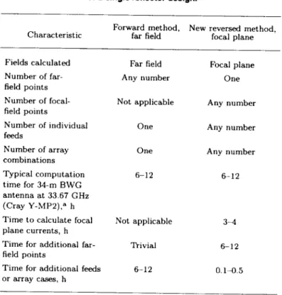
evaluation is only done once for a given scan direction or reflector surface distortion for all array feed geometries and types considered. Table 1 tabulates the relative merits of focal region analysis (sometimes referred to as reverse or receive scattering) and far-field analysis (sometimes referred to as forward or transmit scattering). A rough rule of thumb is that any analysis that requires evaluating the radiated fields at a number of far-field observation points is best done with conventional far-field analysis. How-ever, analysis that requires investigating many different feed or array feed designs is accomplished faster and more easily by using focal plane analysis.

Examples are given using the technique to design an array feed for the correction of gravity-induced distortions of a large dual-shaped ground antenna, both conventional and beam waveguide (BWG), and to design an array feed for improved wide-angle scan. The main emphasis of the examples, however, is on beam-waveguide designs as exemplified by the Deep Space Network (DSN) Deep Space Station (DSS)-13 34-m antenna at Ka-band (33.67 GHz).

Table 1. Comparison of antenna computational techniques for a single reflector design.

Forward method, New reversed method,

Characteristic far field focal plane

Fields calculated Far field Focal plane

Number of far- Any number One

field points

Number of focal- Not applicable Any number

field points

Number of individual One Any number

feeds

Number of array One Any number

combinations

Typical computation 6-12 6-12

time for 34-m BWG antenna at 33.67 GHz (Cray Y-MP2), a h

Time to calculate focal Not applicable 3-4

plane currents, h

Time for additional far- Trivial 6-12

field points

Time for additional feeds 6-12 0.1-0.5

or array cases, h

a Due to priority restrictions for large jobs, turnaround times can be more significant than actual computational times.

II. Focal Plane Analysis

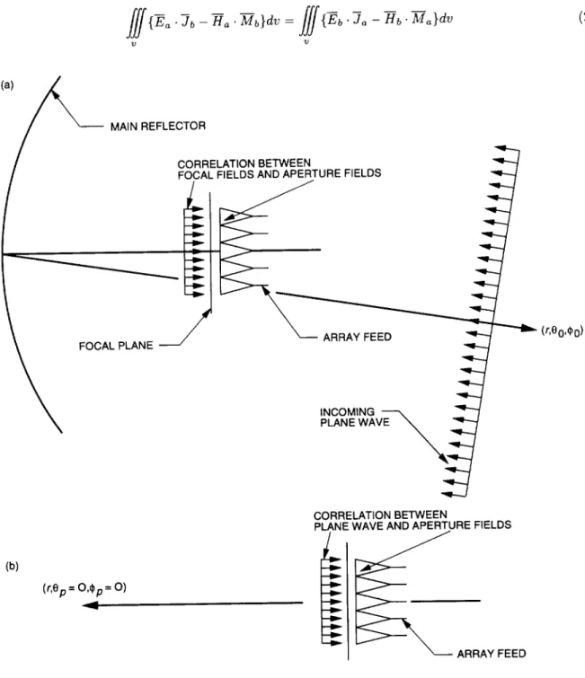
The calculation of the gain of an antenna system, using the antenna focal plane analysis technique, can be illustrated by a simple single-reflector antenna, as shown in Fig. 1. Referring to Fig. l(a), the first phase of the analysis consists of several steps. First, the focal-plane fields produced by a plane wave impinging upon the reflector antenna aperture are computed. Second, the aperture fields of the feed horns located at the focal plane are determined, and these fields are then convolved with the focal plane fields to provide a set of complex feed weights. The process can be explained as follows: Consider a reflector antenna fed by a horn. We wish to determine the gain of this system in a given direction, (00, ¢0), in the receive mode. First, consider the Lorentz reciprocity theorem:

--//{'-Za x "-Hb--'-Eb X -'Ha}.d--s -._ f// {F-'a " gb-- Ha" Mb - Eb" Ja J- gb" Ma} dU

8 v

(I)

In this expression, Ea and Ha are fields radiated by a set of sources Ja and Ma, and also Eb and Hb are fields radiated by sources 75 and Mb. The left integral is over a closed surface that encloses the volume defined by the integral on the right side. Over an infinite region, the surface integral becomes zero. The Lorentz reciprocity theorem can, therefore, be rewritten as

/f {Ea. Jb-- Ha • Mb}dV = /f/{Eb" Ja - Hb. Ma}dv

1} v

(2)

MAIN REFLECTOR

CORRELATION BETWEEN

FOCAL FIELDS AND APERTURE FIELDS

FOCAL PLANE J ARRAY FEED

INCOMING PLANE WAVE (r, e0,¢0) (b) (r,ep: O,¢p = O) CORRELATION BETWEEN

PLANE WAVE AND APERTURE FIELDS

i l ARRAY FEED

Fig. 1. Focal plane analysis geometry: correlation between (a) focal fields and aperture fields and (b) plane wave and aperture fields.

which says that, as long as the relationship between the fields and their source currents holds true, the results will be the same wherever the integrals are evaluated in the region. Let us redefine the a sources

as sources Jha and Mha, to be associated with the feed horn apertures and generating the fields -Eha and

Hha in the aperture plane of the feed. In turn, let us redefine the b sources as sources PIp and Mfp, to be associated with the antenna reflector system when illuminated by an incident plane wave source from a direction (00, ¢0) and evaluated in the reflector system focal plane. The feed horn apertures are defined to be coplanar with the antenna focal plane.

Since the integration is limited to the aperture plane/focal plane, the integrals reduce to surface integrals. Each integral is proportional to the feed-horn output voltage [1]. The left-hand equation is used in this work since the program that generates the focal-plane equivalent currents outputs currents and the program that computes the feed-horn aperture distributions outputs fields. The expression relating the feed-horn outputs, v_, to the currents from the antenna reflector system and the feed-horn aperture fields is then

-- i

The Eha and Hha should be determined in the presence of the antenna reflector system, and the focal plane currents -Jfp and M/p should be obtained when the feed horn is present. Such computations

would require that the interactions between the feed horns and the reflectors be taken into consideration. Taking into account_ these__interactions seriously complicates the analysis and increases the computational time. Often Eha and Hha are approximated to the aperture fields of a horn radiating into an infinite

homogeneous free space (no reflector), and the focal-plane currents J:p and M/p of the antenna reflector system are also obtained in the absence of a feed. This is a reasonable assumption when the feed and antenna reflector system are widely separated in terms of wavelengths.

As will be seen later, there is also a need to obtain the performance of a feed horn in the presence of a plane-wave incident field arriving from a direction (Op, Cp) and in the absence of the antenna reflector system, Fig. l(b). In the same manner as presented above, it can be shown that the output voltage for such a feed horn is

v_,. o¢ j/ {-Eh_ " -Jp,_ - -Hh,_ " -Mp_, }ds (4)

8

where gpw and Mpw are the currents in the feed aperture plane due to the incident plane wave field. In Eqs. (3) and (4), the proportionality constants should be the same, being a function of the horn aperture characteristics. The proportionality constants can be eliminated by performing the ratio of Eqs. (3) and (4) as follows:

ff {-Eh_"--J:p - -Hh_' M :p }ds

"UrA s

v,,---_,

= ff {-Eha"-J,,w - -Hh_ "Mpw }ds

(5)

Let us now consider two transmit situations. First, let the feed horn radiate in the absence of the antenna reflectors and let the radiated field at (r, 0p, Cp) be Eh and the power be Po. Then the gain of the feed horn in the direction (Op, Cp) is

Gh = --_-IEhl 2

(_)

t'o_?

Next, let the horn illuminate the reflector system. The scattered field at (r, 0o, ¢o) is Ea. Assume that the power that is radiated by the feed horn is still Po. Then the gain of the complete antenna system in the direction (00, ¢0) is Ga -- 4_r2 lea[ 2 (7)

vPo

Go = Gh IE°[_

(S)

[Eh[2

From reciprocity, we know that the radiated fields and horn output voltages are related by

IE_l2

Iv_l 2

IEhl_ -I_.1

_

(9)

Therefore, by combining Eqs. (5) and (9), the overall gain of the reflector antenna system can be found in the receive mode from

Ga = Gh "

Iff{-Eho. Tip - -gho" _p}dsl

8

(10)

It should be noted that (0o, ¢0) and (0p, Cp) need not be the same. Therefore, (0p, Cp) has been set to (0.0, 0.0) for simplicity of analysis when evaluating the interactions of the array feed with an incident plane wave and computing the feed horn far-field gain, Gh.

III. Optimization Technique

The optimization technique used in obtaining the maximum gain for an antenna reflector system illuminated by a group or an array of feed elements is referred to as the conjugate weight or match method [2]. Consider a reflector antenna with an array feed operating in the transmit mode and with each feed element excited with equal signal levels. In some direction (00, _b0), in which the maximum output fields are desired, the output field for each feed element is determined. Let fi represent the complex output field voltage of the antenna for feed element i in the direction (0o, ¢0). Then the maximum or optimum output field in that direction would be

N

_=I

If in the receive mode, ci is the output voltage from the ith feed element of the reflector antenna system, when illuminated with a plane wave arriving from the direction (00, ¢0); then the total received signal

N

E"

v_ = cic _ (12)

i=l

From reciprocity, ci/fi = const for all i. Therefore, except for a constant, the expressions that are based on the complex weighting in the receive mode are identical to those in the transmit mode. Thus, vr

also represents an optimum gain solution. In this analysis, the effects of mutual coupling between array elements have been ignored. For the size and type of feed elements considered in this study, this is not a limitation.

If the integral portion of Eqs. (3) and (4) are rewritten as follows,

Ci : //{Ehai "-Jfp - -'Hhal " J_--Tfp}ds (13)

di = //{-Eha, •-Jp,_, - -Hha, •-Mpw}ds (14)

$

by the use of Eq. (12), Eq. (10) can be rewritten as

N 2

1

Ga = Gh " 5=1N (15)

i=1

This expression is used to determine the optimum antenna gain simply by knowing the focal plane currents of the antenna, the array feed geometry, and the feed element aperture fields. The gain of the array feed in the absence of the antenna reflectors, Gh, is obtained by first performing a physical optics integration over the Eha fields in each feed element aperture to obtain the far-field pattern for each element. Then the power and peak fields are computed from the total fields from all elements in the conventional manner and used to compute Gh.

The analysis method consisted of computing the focal plane currents of a reflector system using reverse (receive-mode) scattering programs. Physical optics is used for a single-reflector antenna design and a combination of geometrical optics off of the main reflector and physical optics off of a subreflector is used in a dual-reflector antenna system. Both electric and magnetic focal plane currents are computed on a fixed grid over which the array-feed element aperture distributions are superimposed. This grid becomes the integration grid over which the convolution of the focal plane currents and feed aperture field distributions are integrated. The feed aperture fields are in effect interpolated to fall on the points established by the reverse scattering program's focal plane grid. To generate the feed element aperture fields at the required grid locations, the far field element patterns are expanded into a set of circular waveguide modes. These modes can then be evaluated at the required grid locations to obtain the feed aperture fields.

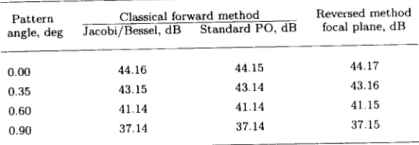
IV. Accuracy

Considerations

To determine the accuracy of the focal plane technique, the gain of a single reflector antenna was calculated using three different approaches: (1) the focal plane technique combined with a physical optics program that took a plane wave impinging on the reflector and computed the required focal plane currents,

(2) a forward scattering program, using a physical optics technique that made use of the Jacobi/Bessel series to describe the output fields [3], and (3) a forward scattering program, using a physical optics method that used a triangular integration grid [4]. The gain pattern was calculated for a number of far-field observation points. Obviously, for the forward approach, this simply meant specifying the locations of the observation points. For the focal plane approach, however, calculating the gain pattern required the incoming plane wave direction to be adjusted such that the direction of propagation was from the observation point. Table 2 summarizes the results. As can be seen, all three techniques agreed within

a few hundredths of a dB for pattern gain variations of 7 dB. The only precautions needed to get this accuracy were to make sure sufficient integration points were used and that all series representations of fields had converged.

Table 2. Accuracy of the focal plane method, antenna gain.

Pattern Classical forward method Reversed method

angle, deg Jacobi/Bessel, dB Standard PO, dB focal plane, dB

0.00 44.16 44.15 44.17

0.35 43.15 43.14 43.16

0.60 41.14 41.14 41.15

0.90 37.14 37.14 37.15

V. Use of Optimization

to Minimize

Beam Scan Loss

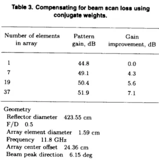
One application of the optimization approach described in this article is to minimize the scan losses of an antenna where the antenna beam has been scanned off the axis of symmetry by a laterM displacement of the feed system. Depending on the size of the displacement, the losses can be quite large, due to the optical aberrations produced. The test case used consisted of a 423.55 cm-diameter parabolic reflector with a focal length-to-diameter ratio (F/D) of 0.5. The compensating array feed consisted of up to

37 elements. The main beam was scanned 6.15 deg off the axis of symmetry to produce a scan loss on the order of 8 dB. The primary array element that produces the specified beam scan was located 24.36 cm off the antenna axis. The antenna parameters and the improvement in performance due to array feed optimization is shown in Table 3. The gain for several numbers of array elements is shown. The gain for an antenna with the single-feed element is 44.8 dB. With complex conjugated weights applied to 37 elements, the gain is increased to 51.9 dB for a net improvement of 7.1 dB.

VI. Compensating

Reflector

Distortions

by Optimization

As was mentioned in the introduction, the main purpose of the focal plane optimization technique was to reduce the amount of computer time required to optimize the design of an antenna system to

maximize the gain. This is particularly true for studying large, complex antennas such as the 34-m beam-waveguide dual-shaped reflector antennas, operating at 33.67 GHz, that are used at the Jet Propulsion Laboratory/NASA deep space tracking network. However, a second advantage of the focal analysis is that it allows the actual focal field distributions to be displayed. This can many times give some insight into why the antenna behaves the way it does. In the conventionM far-field optimization approach [5], a full scattering calculation is required for each array feed element, for each antenna configuration, and for each array geometry. In the focal plane analysis, a scattering calculation is required only for each antenna configuration. Any number of array geometries and any number of feed elements can be studied without any further scattering calculations.

Although considerable effort was expended to develop the focal plane analysis technique, the main purpose of the study was to determine the properties of a shaped antenna illuminated by an array feed

Table 3. Compensating for beam scan loss using conjugate weights.

Number of elements Pattern Gain in array gain, dB improvement, dB

1 44.8 0.0 7 49.1 4.3 19 50.4 5.6 37 51.9 7.1 Geometry Reflector diameter 423.55 cm F/D 0.5

Array element diameter 1.59 cm Frequency 11.8 GHz

Array center offset 24.36 cm Beam peak direction 6.15 deg

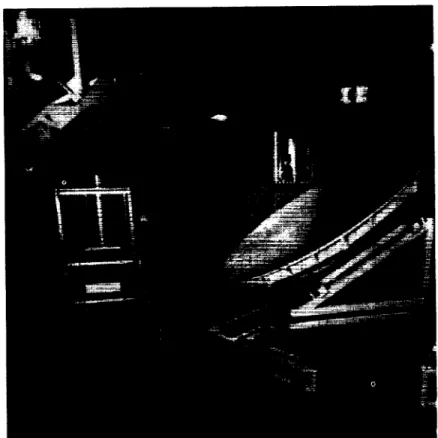
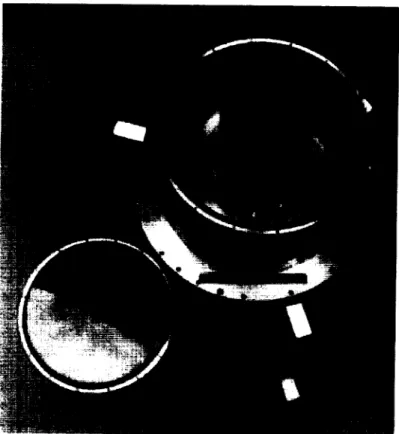
where the array feed's purpose is to compensate for various antenna aberrations or distortions. The focal plane technique is simply the enabling technology. A conjugate weighting technique is used to determine the excitation weights for each array feed element so that the antenna losses might be recovered. The goal was to compensate the antenna for gain losses that resulted from gravity-induced distortions as a function of the antenna's elevation angle, where the surface is adjusted for minimum distortion at a 45-deg elevation angle. The main application is for a beam-waveguide (BWG) antenna where the array feed system is mounted in a room below the antenna. However, to expedite the validation of the focal plane analysis technique, the initial calculations were limited to the main focal plane of the antenna, i.e., no BWG. Figure 2 illustrates the geometry of the DSS-13 34-m BWG antenna, the properties of which were made the basis of this study. The frequency used was 33.67 GHz. Of particular interest is the focal region at F1, where the initial calculations were made. A second set of calculations was made at F3, the focal region created by the beam-waveguide system in the basement or pedestal room of the antenna. Although the beam-waveguide system consists of two parabolic mirrors, one elliptical mirror, and three plane mirrors, only the three curved mirrors are included in the analysis. The three plane mirrors, if properly sized, should not affect the performance of the antenna system. Figure 3 shows an array feed with the RF front-end setup at F3 that was used in another study for an experimental evaluation of using array feeds to compensate for antenna distortion losses. Figure 4 shows a seven-element array, with 4.45-cm diameter dual-mode horns, used in the experimental system. This illustrates a typical application for the results of the trade-off study discussed later in this article.

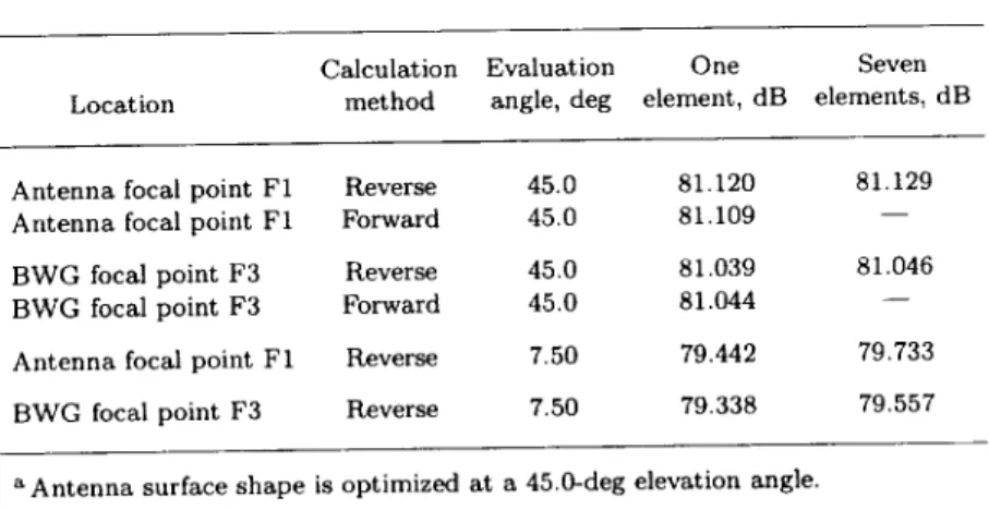
A summary of results at F1 and F3 for 7.5- and 45-deg elevation angles is shown in Table 4. The results are based on the use of optimum feed horn sizes and focus. Both the focal plane or reversed scattering method and the forward or conventional scattering method were used. The results for the forward method are from an optimization study done at the time DSS 13 was completed. As can be seen, the results for the forward and reversed approaches are very close.

A. Optimization at F1

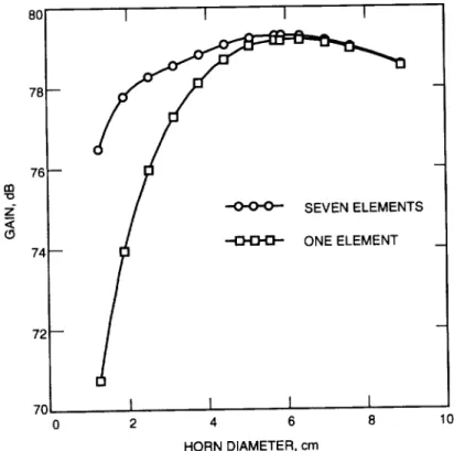
The case used for the evaluation consisted of an array feed of seven equally sized elements in a circular cluster on a triangular grid. The first step was to select an element size that minimized the antenna loss at one of the distortion extremes, such as at an elevation angle of 7.5 deg. A set of 13 element diameters was selected, ranging from 2 to 13 cm. For each element diameter, the focal plane optimization technique was used to determine the feed element weights that gave the best performance improvement. Figure 5 contains two curves. The first curve shows the performance of the antenna that results from a single

TRIPOD 34-m SHAPED-SURFACE REFLECTOR SHAPED-SURFACE SUBREFLECTOR I I F1 F2 F3 BEAM WAVEGUIDE TRACK MICROWAVE TEST PACKAGE ;UBTERRANEAN PEDESTAL ROOM

Fig. 2. DSS-13 34-m beam-waveguide antenna.

Fig.4. A

.-o--o-o- SEVEN ELEMENTS

_// _ ONE ELEMENT

[] I I I ] I

2 4 6 8 10 12 14

HORN DIAMETER, cm

Fig. 5. Optimum antenna gain versus feed element diameter (7.5-deg elevation angle).

Table

4.Gaincomparisons

forashaped

antenna

between

BWG

and

non-BWG

designs

using

focalplane

orfar-field

analysis,

Location

Calculation Evaluation One Seven

method angle, deg element, dB elements, dB

Antenna focal point F1 Reverse 45.0 81.120 81.129

Antenna focal point F1 Forward 45.0 81.109

--BWG focal point F3 Reverse 45.0 81.039 81.046

BWG focal point F3 Forward 45.0 81.044

--Antenna focal point F1 Reverse 7.50 79.442 79.733

BWG focal point F3 Reverse 7.50 79.338 79.557

a Antenna surface shape is optimized at a 45.0-deg elevation angle.

on-axis element as a function of element size. The second curve shows the best performance for an array of equally sized elements. From the curve, it was found that an array of elements with diameters of 9.26 em gave the best performance at an elevation angle of 7.5 deg. Calculations using the optimization technique were repeated for a series of antenna elevation angles, using the 9.26 cm-diameter elements, to determine the best performance that can be obtained with the optimum element size determined at 7.5 deg. Figure 6 summarizes the result. The first curve illustrates the performance that would be expected due to reflector distortions as a function of elevation angles if a single feed horn were used. The second curve shows the improvement in performance that can be obtained with the seven-element array

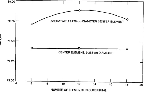
using the optimum element weights computed by the optimization technique. The maximum improvement at an elevation angle of 7.5 deg is 0.29 dB out of a distortion loss of 1.68 dB. It was found that if the number of elements in the ring around the center element was increased from 6 to about 12 elements, an additional improvement of 0.18 dB could be obtained for an overall improvement of 0.47 dB (Fig. 7).

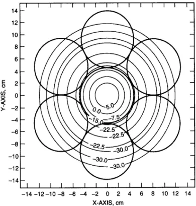
As indicated earlier, the availability of the focal plane fields from the focal plane analysis program can give an insight into why the antenna performs the way it does. Figure 8 shows the focal plane field distribution at F1 for an elevation angle of 45 deg. Overlaying the field distribution are the outlines of the optimum-size feed horns. As can be seen, the center horn covers the field distribution from in excess of 5.0 dB down to almost -15.0 dB. The outer ring of feed horns covers a region of ripples indicated by the multiple contour rings at -22.5 and -30.0 dB. These multiple rings also indicate that phase reversals are present in the region of the outer horns. Thus, the center horn captures the majority of the focal plane fields, whereas the outer horns couple very little of the fields because of the low field strengths and the fact that the phase reversals will cancel out a large part of what field levels are available. Hence, the outer elements will not improve the antenna performance, as can be seen in Fig. 6. Figure 9 is a similar plot for an elevation angle of 7.5 deg. In this case, the center horn captures less energy since the peak level has dropped and the contour associated with the edge of the horn aperture is now only -5.0 dB. Although the outer ring of horns covers a region of levels primarily between -5.0 and -25.0 dB, which appears to represent the majority of the energy missed by the center horn, as is seen in Fig. 6, only a small part of the lost energy was recovered at 7.5 deg. This is due to the fact that the typical feed-horn

aperture distribution is Gaussian and couples the most energy when associated with a Gaussian focal plane distribution, such as is seen in Fig. 8 for the center horn for the 45-deg elevation case. In the case of the outer horns at 7.5 deg, the focal plane distribution they see is essentially wedge shaped in a radial direction and, therefore, these horns are very inefficient in coupling the energy within their apertures.

A question raised during the study was whether the array feed could recover losses due to diffraction from the subreflector support tripod. Calculations were made to address this question at an eleva-tion angle of 45 deg. To simplify the calculation and to avoid developing a special program to compute

m .lo < L9 80.! 80.(

I

I

I

I

I

I

I

I

'--O.--O--O--- SEVEN ELEMENTS

'_E)'-O--O-- ONE ELEMENT

I

I

I

I

I

I

I

10 20 30 40 50 60 70 80 9O

ELEVATION ANGLE, deg

Fig. 6. Optimum antenna gain versus antenna elevation angle (9.26-cm horn diameter).

rn 10 z ,< 80.00 79.75 79.50 79.25 --79.00 4

I

I

I

I

I

I

I

CENTER ELEMENT, 9.258-cm DIAMETER

[]

I

I

I

I

I

I

I

6 8 10 12 14 16 18

NUMBER OF ELEMENTS IN OUTER RING

Fig. 7. Antenna gain versus number of elements In outer rlng (7.5-deg elevation angle).

20

I I I I I I I I I I I I I I I 14- 12- 10-8 6 4 E 2 tO

-_

0

Fig. 8, Focal plane field distribution overlaid with the

outline of the 9.258-cm diameter horns at F1 for a 45-deg

elevation angle, 14 12 10 8 6 4 E 2 tO u_ - 0 _- -2 --4 --6 -8 -1( -1: -14 -14-12-10-8 -6 -4 -2 0 2 4 6 8 10 12 14 X-AXIS, cm

Fig. 9. Focal plane field distribution overlaid with the

outline of the 9.258-cm diameter horns at F1 for a 7.5-deg

the diffraction from the support tripod, the decision was made to project the tripod blockage onto the main reflector similarly to that done with holography. In the area of the projected blockage, the main-reflector surface currents were set to zero. Using the physical optics scattering program, the fields on the subreflector were then computed. Using the reverse scattering program, the focal plane currents in turn were computed from the subreflector currents. Using the focal plane analysis, the gain of the antenna with support tripod blockage was determined. As a reference, the gain for no blockage was calculated using the same technique. For one horn, the loss (or difference in gain) due to blockage was 0.44 dB. For an array of seven horns, again the loss due to blockage was 0.44 dB. The array provided an improvement on the order of 0.01 dB for both with and without blockage. Therefore, the array was incapable of recovering blockage losses, and the calculated losses were due to the support tripod scattering fields outside of the region occupied by the array.

B. Optimization at F3

The major part of the study was done with the array feed located at F3 since this location would be used for a practical implementation. The design approach used followed that used at F1, where first the gain as a function of horn diameter was calculated. This was done at one extreme elevation angle, such as 7.5 deg, rather than at 45 deg, so as to optimize the array design at the point where the losses would be the greatest. This calculation was done at two axial focal positions of 0.0 and -8.89 cm from F3 so as to bracket the optimum focal position. Figures 10 and 11 illustrate the results for an array of seven horns, where the best horn diameter for a focal position of 0.0 cm was 5.88 cm, and, for a focal position of -8.89 cm, the best diameter was 5.08 cm. Next, the calculations were repeated as a function of the axial focal position, where the horn diameters were linearly interpolated at each focal position using the two best horn diameters previously calculated at the bracketing focal positions. The calculations were done at elevation angles of 7.5 and 45 deg. In Figs. 12 and 13, it is seen that the performance for an array of seven horns peaks at focal positions of -6.67 cm for an elevation angle of 7.5 deg and -6.1 cm for an elevation angle of 45 deg. Since the gain is quite flat in the vicinity of the best focus, a focal position between the best focal position for the two elevation angles was selected as the focal position for the remainder of the calculations. The selected axial focal position is -6.35 cm for a horn aperture diameter of 5.31 cm.

Having selected the nominal location for a seven-horn array and the best central horn diameter, the rest of the study consisted of varying the various parameters of the array design. Figure 14 shows the antenna performance as a function of elevation angle for the center horn only and for an array of seven horns. At an elevation angle of 45 deg, the center horn and the array have the same performance, as expected, since the antenna surface was adjusted at this angle. At an elevation angle of 7.5 deg, the single-horn performance shows a loss of 1.70 dB relative to the performance at the 45-deg elevation angle. Using the array to recover this loss of performance, only a 0.22-dB improvement was obtained. Earlier calculations using the forward or transmit mode to compute the possible performance improvement showed improvements of about 0.4 dB. The earlier calculations used the array geometry that was used in an experimental program, where the array horn diameters were not optimized and the horns were operated 1.67 GHz away from their design frequency, allowing more room for improvement. In this study, the horn size was optimized, as discussed in the previous paragraph.

The calculation in the first paragraph of this section was for a seven-horn array, where the center horn and the six horns in a ring around the center horn had the same diameters. The next calcula-tion investigated the effect of using different numbers of horns in the ring around the center horn and adjusting the diameter of these horns to completely fill the ring. The larger the number of horns in the rings, the smaller the horn diameters. Figure 15 illustrates the performance for this case. In the figure, the performance of the center horn is included as a baseline and is a straight line since it is not affected by the number of outer-ring horns. Also, the figure shows calculations for one outer ring and two outer rings. Where two rings are used, both rings have the same number of horns," the second ring nest-ing in the first ring. This necessitates the horns in the second ring being larger than those in the first ring.

nn "ID < rn m ,< 8O 78 7_ 74 72 7C 8O 78 76 74 72 7O I I I I TS m

I

I

I

I

Fig. 10. Antenna gain versus horn diameter, z (focus) = 0.0 cm

(7.5-deg elevation angle).

I I I I

l -O-O-O--O.--O-O- SEVENONE ELEMENTELEMENTS

I

I

I

I

2 4 6 8

HORN DIAMETER, cm

10

Fig. 11. Antenna gain versus horn diameter, z (focus) = -8.89 cm

81

•-o-o-o-- SEVEN ELEMENTS

-.O.-,13.-O- ONE ELEMENT

I I I I

-8 -6 -4 -2

Z-FOCUS, cm

Fig. 12. Optimum antenna gain versus z (focus) at F3,

7.5-deg elevation angle (optimum horn diameter).

rn z ,< (_ 81.5 81.0 --80.! --80.( --79.5 n 79.0 78.5 -10

I

I

I

I

-O-O-O- SEVEN ELEMENTS

•-D.,O-O- ONE ELEMENT

I

I

t

I

-8 --.6 -4 -2 0

Z-FOCUS, cm

Fig. 13. Optimum antenna gain versus z (focus) at F3,

45-deg elevation angle (optimum horn diameter).

81.5 I I t I I I m (.9

_z

ELEVATION ANGLE, deg

80.25 80.00 79.75 79.50 79.25 79.00

Fig. 14. Optimum antenna galn versus elevation angle (z (focus) =

-6.35 cm, horn diameter = 5.309 cm). I I I I I O SECOND RING A FIRST RING [] CENTER ELEMENT I I I I I 4 8 12 16 20

NUMBER OF ELEMENTS PER RING

Fig. 15. Antenna gain versus number of array elements per rlng (z (focus) = -6.35 cm, horn dlameter = 5.309 cm, elevatlon angle = 7.5 deg).

For one ring of six horns, the improvement was 0.22 dB, as shown before. However, if the number is increased to eight horns, the improvement jumps to 0.63 dB and then drops off for a larger number of horns. Using 2 rings, an improvement of 0.72 dB can be gained for 12 horns in each ring. However, using the second ring, which implies a 25-horn array, only gives an improvement of 0.09 dB over the single-ring case, which is a 9-horn array. Therefore, the use of a second ring is not practical considering the increased complexity. The reason that increasing the number of horns makes an improvement can be seen by reviewing the focal plane distribution. Figure 16 shows the focal distribution overlaid with the outline of the 5.31-cm diameter horns in the seven-horn case. It can be seen that the center horn encompasses the region where the fields are best behaved. The horns in the outer ring, however, are so large that they cover an area where the fields slope across the aperture from -5 to -35 dB and, therefore, do a poor job of coupling the fields. The horns like to see a Gaussian distribution for best performance. Figure 17 shows the focal distribution overlaid with the outline of the horns for the eight horns-per-row case, where the center horn is 5.31 cm in diameter. Here the smaller horns in the first row do a better job of sampling the fields since the fields do not vary more than 10 to 15 dB across their apertures. The horns in the second row, however, cover regions where the fields are not well behaved and recover very little of the field energy. This case shows that increasing the number of horns by two can cause a significant improvement. However, it should be noted that the array geometry is driven by the focal distribution, which is unique for a given antenna system design and associated aberrations and, therefore, the results could be significantly different for other antenna designs. This case is interesting because it is an example of the type of cases that are amenable to the focal plane analysis technique.

In an earlier study, ray tracing techniques were applied to a seven-horn array, using the same geometry used in this article. It was found that with all the array horn axes parallel to each other at F3, at their image point at F1, the beams associated with the horns in the ring around the center horn pointed away from the antenna axis. This could be likened to an array located at F1 having all but its center horn rotated outward from the antenna axis. The effect is to improperly illuminate the antenna subreflector. At F3, it was found that by rotating all but the center horn inward by 2.62 deg in an aberration-free environment, all the beams at F1 could be made to be parallel. Another way of viewing this situation is that the phase patterns of the focal field distribution at F3 for a BWG antenna are not uniform, but tapered. The horns need to be rotated to better match the focal plane phase distribution. Since with optimum horn diameters the outer horns are only useful in the presence of antenna aberrations, it was of interest to see if rotating the horns could help in recovering more of the losses due to aberrations. At an elevation angle of 7.5 deg, a series of calculations was made, rotating all but the center horn inward. In Figure 18, it is shown that, for a seven-horn case, rotating the horns 5.2 deg inward improved the performance by 0.46 dB. A similar calculation was made for the case that had the optimum eight horns in the ring (nine-horn array). In this case, rotating the horns about 4.0 deg had little effect. Evidently, significant phase variations in the focal region were beyond the area covered by the smaller outer horns for the nine-horn array, but were within the region covered by the larger outer horns of the seven-horn array. Figure 19 shows the performance as a function of elevation angle for the seven-horn case, with the horn rotation angle set at 5.2 deg.

There are some asymmetries in the BWG geometry that are not significant to horns mounted on the antenna optical axis, but could be of concern for off-axis horns such as are used in an array feed system. Of concern was what effect these aberrations might have on the array performance as a result of a rotation of the antenna in azimuth. Azimuthal rotations cause a change in the relative rotational position of one

section of BWG mirrors to another. Figure 20 shows the antenna performance at an elevation angle of 7.5 deg as the antenna rotates in azimuth. For the center horn only, the variation is only 0.04 dB, which is negligible. For the array, the variation is 0.13 dB, still not significant. The other issue is what happens when the array is rotated about its axis at F3. Does this affect the way the outer horns sample the focal fields? For example, is there an optimum angle? Calculations made on the 10-horn array showed variations on the order of 0.1 dB.

7 6 5 4 3 2 E 1

0--" 0

._2

Fig. 16. The focal distribution overlaid with the outline of the horns for the seven-horn case (z (focus) = -6.35 cm, elevation angle = 7.5 deg, horn diameter = 5.309 cm).

-7 -6 -5 -4 -3 -2 -1 1 2 3 4 5 6 7

X-AXIS, cm

Fig. 17. The focal distribution overlaid with the outline of the horns for the eight horns-per-row case (z (focus) = -6.35 cm, elevation angle = 7.5 deg, horn diameter = 5.309 cm).

80.00 79.80 79.60 z" 79.40 79.20 79.00 81.5 81.0 80.5 z" 80.0 (.9 79.5 79.0 78.! 0 I I I I I I D [] ONE ELEMENT I I I I I I -2 0 2 4 6 8 10 12

HORN POINTING ANGLE, deg

Fig. 18. Antenna gain versus horn pointin_i angle (z (focus) = -6.35 cm, elevation angle = 7.5 deg, horn diameter = 5.309 cm).

I I I I I I

O SEVEN ELEMENTS O ONE ELEMENT

I I I I I I

10 20 30 40 50 60

ELEVATION ANGLE, cleg

Fig. 19. Antenna gain versus elevation angle (horns pointed) (horn angle = 5.2 deg, z (focus) = -6.35 cm, horn diameter = 5.309 cm).

70

a] z < 79.7 79.6 79.5 I I t O SEVEN ELEMENTS [] ONE ELEMENT 79.4_,_ 79.31 0 I I I 90 180 270 360

ANTENNA AZIMUTHAL ANGLE, deg

Fig. 20. Antenna gain versus antenna azimuthal angle (z (focus) : -6.35 cm, elevation angle = 7.5 deg, horn diameter = 5.309 cm).

Figures 21 and 22 display the focal plane fields for the antenna and are provided for general interest. Figure 21 shows the focal fields for antenna elevation angles of 7.5, 22.5, and 45 deg at the optimum axial focal position of -6.35 cm. The primary effect of elevation angle-induced distortions on the focal plane distribution is a lowering and spreading of the fields. At 45 deg, the field distribution is approximately rotationally symmetric. At F1, the distribution is perfectly circular, as is seen in Fig. 8. The lack of perfect circular symmetry shown in Fig. 21(c) is due to the effects of the BWG. Figure 22 shows the effect of axial focus changes on the focal fields at an elevation angle of 7.5 deg. There appears to be a rotation in the structure of the focal fields in the vicinity of the distribution main lobe as the focus is changed. Figure 22(b) shows the best focal position, where the array position is -6.35 cm.

VII. Analysis of Experimental Configuration

An experimental program, supported by another task, was performed at DSS 13 using a seven-horn array located at F3 that had the same geometry as used in this study, with one exception: The array

horns were restricted to a nonoptimum diameter of 4.45 cm. Another difference is the dual-mode horns used in the experiment were designed for 32.0 GHz but operated at 33.67 GHz. This change in frequency degraded the pattern properties of the horns. Because of the degraded horn performance, the results presented in the previous section are not typical of what would be expected from the experimental program. To provide better predictions, different horn-mode models were developed to account for the change in performance. While the ratio of the TMm mode to the TErn mode was 0.405 for the dual-mode horns used in this study, to model the horns in the experimental program, a mode ratio of 0.206 with a phase of -71.73 deg was required.

Calculations were made to determine the best axial focal position for the array. Figure 23 shows the results for an elevation angle of 7.5 deg. For a single horn, the best position was -7.62 cm, and for

7L _ _ I1j._+ i _L_l _ , J _/ -7 -6 -5 -4 -3 -2 -1 0 1 2 3 4 5 6 7 X-AXIS, cm E t_ ¢fi >-7 6 5 4 3 2 1 0 -1 -2 --3 -4 -5 -6 -7 I I I I I I I I I I I -7 -6 -5 -4 -3-2 -1 0 1 2 3 X-AXIS, cm I I I (b) I/I I-4 5 6 7 III IIIII111111 -' _-5 _ _-2 -1 0 1 2 3 4 5 6 7 X-_lS, cm

Fig. 21. The focal fields for antenna elevation angles of (a) 7.5, (b) 22.5, and (c) 45 deg (z (focus) = -6.35 cm).

a seven-horn array, the best position was -8.89 cm. Figure 24 shows results for an elevation angle of 45 deg, and, for both the single horn and for the array, the best focal position is -7.62 cm. Since the focus curve is essentially flat in the region of -8.0 cm and the experimental measurements were made at -8.89 cm, the predictions were calculated at -8.89 cm. Figure 25 shows the antenna gain as a function of elevation angle. At an elevation angle of 45 deg, the gain is 80.66 dB for a single horn and 80.70 dB for the array, for an improvement of 0.04 dB. At an elevation angle of 7.5 deg, the gain is 78.89 dB for a single horn and 79.39 dB for the array, for an improvement of 0.50 dB as compared with a loss due to surface distortions of 1.77 dB.

To determine if rotations of the antenna in azimuth would affect the performance of the array at F3, a series of calculations was made, where the azimuthal position of the antenna was changed in increments

7 6 5 4 3 2 _. -1 -2 -3 -4 -5 -6 -7 E o cB 7 6 5 4 3 2

1

Fig. 22. The effects of axial focus changes on the focal fields at an elevation angle of 7.5 deg: (a) z = 0.0 cm, (b) z = -6.35 cm, and (c) z = -8.89 cm.

of 45 deg. For an elevation angle of 45 deg, the variation is 0.02 dB for both the center horn and the array. The performances for both the center horn and the array are the same since, at an elevation angle of 45 deg, the outer horns have very little effect. The variation in performance at an elevation angle of 7.5 deg is 0.03 dB for the center element and, for the array, 0.13 dB. To determine the best rotational alignment of the array at F3, the array was rotated about the optical axis at F3 in fractions of the angle subtended by the width of a horn aperture in the ring surrounding the center horn. A series of calculations

in effect would rotate one horn into the position previously occupied by the next horn in the ring before the calculations began. For an elevation angle of 7.5 deg, the gain of the array varied by 0.16 dB. For optimal results, the array should be rotationally adjusted.

nn < L9 03 '10 .< L9 81.0 80.5 --80.0 --79.5 --79.0 --78.5 --78.0 --10 81 .I 80.! -80. --79.5 --79.0 --78.5 --78.0 -10 I I I I O SEVEN ELEMENTS [] ONE ELEMENT O

I

I

I

I

Fig. 23. DSS-13 antenna gain versus z-focus at F3, 7.5-deg elevation angle.

I I I I O SEVEN ELEMENTS [] ONE ELEMENT

I

I

I

I

Fig. 24. DSS-13 antenna gain versus z-focus at F3, 45-deg elevation angle.

81.0 I I I I I I rn -o z ,< (.9 80.5 80.0 79.5 79.0 78.5 13 ONE ELEMENT _

I

I

I

I

I

I

ELEVATION ANGLE, deg

Fig. 25. DSS-13 antenna gain versus elevation angle: focus position, z = -8.890 cm.

7O

VIII. Conclusions

The focal plane optimization technique was shown to provide a method of recovering performance losses for two antenna problems: (1) the aberration losses due to scanning the beam of an antenna and (2) the losses associated with antenna reflector distortions that result from changes in the antenna elevation position. The second case really demonstrates the power of the focal plane analysis technique. For the antenna configuration associated with the second case, it takes 5.6 h on a Cray Y-MP2 computer to perform one forward scattering calculation to determine the far-field pattern for a single-feed horn. The scattering calculation must be repeated seven times to include the effect of each array feed horn for a seven-horn array, requiring 39.2 h per antenna configuration. The time to compute the optimum gain from the far-field patterns for each feed horn is small compared to the scattering calculation time and will be neglected. If the process is repeated for 13 feed sizes, as was done in the example in Section VI.A of this article, a total time of 509.6 h is needed! The computation time required for the focal plane optimization technique can be determined as follows: Assume the time to do the reverse scattering calculation through the antenna and beam-waveguide optical system is the same as for the forward scattering case, or 5.6 h. The time required to calculate the currents in the focal plane to the required resolution is 3.3 h. This gives a one-time total time of 8.9 h, which does not have to be repeated unless the antenna geometry

changes. The time required to perform the focal plane optimization that must be repeated for each feed size or array geometry ranged from 2 min for the smallest feed size to 33 min for the largest feed size and 22.5 min for the optimum feed size. The total time to perform the optimization calculation for all 13 feed element sizes studied was 2.7 h. The grand total time, including the scattering calculations, comes to 11.6 h. Reducing the computation time from 509.6 h to 11.6 h illustrates the usefulness of this technique. The objection can be raised that you do not need to consider so many element sizes to determine the optimum element size. But that is not the issue. There might also be a need to trade off the array geometry and/or the horn type, such as single mode, dual mode, hybrid mode, or any other type. This could result in the need to analyze more cases than the 13 element sizes considered in the example. The

point is that significant time savings can be obtained by doing the optimization in the focal plane for situations where the scattering calculation times are significant, such as is the case for beam-waveguide antennas where five or more scattering surfaces must be considered and where their sizes in terms of wavelengths are very large.

The focal plane approach is very accurate. Agreement between the focal plane or reverse scattering technique and the classical transmit approach was on the order of 0.02 dB.

Acknowledgment

The Cray supercomputer used in this study was provided by funding from the NASA Offices of Mission to Planet Earth, Aeronautics, and Space Science.

References

[1] R. F. Harrington, Time Harmonic Electromagnetic Fields, New York: McGraw Hill, pp. 116-120, 1961.

[2] P. J. Wood, Reflector Antenna Analysis and Design, London, England: Peter Peregrinus Limited, Institution of Electrical Engineers, p. 190, 1980.

[3] Y. Rahmat-Samii, R. Mittra, and V. Galindo-Israel, "Computation of Fresnel and Fraunhofer Fields of Planar Apertures and Reflector Antennas by Jacobi-Bessel Series--A Review," Journal of Electromagnetics, vol. 1, pp. 155-185, April-June

1981.

[4] W. A. Imbriale and R. Hodges, "Linear Phase Approximation in the Triangular Facet Near-Field Physical Optics Computer Program," Applied Computational Electromagnetics Society Journal, vol. 6, no. 2, pp. 74-85, Winter 1991.

[5] P. W. Cramer, "Initial Studies of Array Feeds for the 70-Meter Antenna at 32 GHz," The Telecommunications and Data Acquisition Progress Report 42-104, October-December 1990, Jet Propulsion Laboratory, Pasadena, California, pp. 50-67, February 15, 1991.