Security Issue Timing: What Do Managers Know, and When Do They Know It?

Security Issue Timing:

What Do Managers Know, and When Do They Know It?

Dirk Jenter, Katharina Lewellen, and Jerold B. Warner*

ABSTRACT

We study put option sales on company stock by large firms. An often cited motivation for these transactions is market timing, and managers’ decision to issue puts should be sensitive to whether the stock is undervalued. We provide new evidence that large firms successfully time security sales. In the 100 days following put option issues, there is roughly a 5% abnormal stock price return, with much of the abnormal return following the first earnings release date after the sale. Direct evidence on put option exercises reinforces these findings: exercise frequencies and payoffs to put holders are abnormally low.

*Stanford University and NBER, Tuck School at Dartmouth, and Simon School, University of Rochester, respectively. We are grateful to Nittai Bergman, Kenneth French, Christopher Hennessy, Robert McDonald, Jeremy Stein, Ryan Taliaferro (AFA discussant), Ivo Welch (NBER discussant), Campbell Harvey (the editor), an anonymous referee, and workshop participants at the 2008 AFA Meetings, BYU, Chicago, Columbia, Georgia, LBS, MIT, the 2007 NBER Universities Research Conference, NYU, Rochester, Stanford, UCLA, and USC for helpful comments and suggestions. We would also like to thank David Hadley (Hadley Partners, Inc., formerly of BT Alex Brown), Ajay Khorana (Citigroup), Anil Shivdasani (Citigroup), and David Strasburg (formerly of Goldman Sachs) for valuable industry perspectives.

During the 1991 to 2004 period, many large U.S. firms, including Bank of America, Boeing, IBM, McDonald’s, and Microsoft, sold puts on their own stock. Our study is the first large-scale empirical analysis of these corporate transactions. A put sale can be viewed as a levered bet that the stock price will not drop. Thought of this way, put options offer a unique setting to study market timing by corporations. Our main contribution is to provide strong evidence that large firms successfully time the market with security sales.

Managers can alter investment, financing, and other corporate decisions if and when they believe their firms’ securities are mispriced. While market timing is the subject of an extensive literature (see Eckbo, Masulis, and Norli (2007) and Baker, Ruback, and Wurgler (2007) for surveys), its importance for corporate behavior is hotly debated and still unresolved. Most of the evidence in support of market timing comes from long-horizon event studies that document abnormal returns following equity issues and repurchases. This evidence is difficult to interpret, however. First, there are many motives for these transactions other than market timing, and it is often difficult to distinguish among alternative explanations. Second, measuring abnormal returns over long horizons is problematic, especially given that equity risk may change around stock issues and repurchases because of contemporaneous changes in asset and/or financing structures.

The put option sale setting helps address the issues of both motivation and measurement, and thus provides a cleaner test. Management’s desire to exploit perceived mispricing represents a highly plausible motive for put sales, whereas other motives seem suspect. For example, put sellers tend to be highly profitable and appear to have few needs to raise outside funds. Firms do not announce their put sales and hence do not seem to use them to signal information to the

market. Selling put options increases rather than reduces firm risk, and hence cannot serve as a hedge. Though market timing motives seem highly plausible, we cannot rule out the existence of other reasons to sell puts. Our empirical tests examine whether managers use private information to time put sales, and the tests do not require that market timing be the only motivation.

The put option setting also allows for more precise measurement of abnormal security behavior following the sales. A typical put in our sample has a maturity of only 6 months. The short maturity allows us to focus on short-term stock price effects, reducing the difficulties associated with long-horizon event studies (see Fama (1998) and Kothari and Warner (2007) for overviews). In addition, since put sale programs typically extend over multiple fiscal quarters, we can examine stock returns subsequent to quarters in which firms skip put sales. Finding no abnormal returns after such quarters is further evidence on timing and alleviates the concern that return benchmarks are misspecified. Further, because put sale proceeds are usually small relative to typical debt or equity issues, it is unlikely that apparent abnormal stock returns after put sales reflect changes in asset risk.

A unique feature of our setting is the ability to investigate option exercises and expirations directly. Successful timing implies that fewer puts are exercised and payoffs are smaller than would be expected in the absence of private information. To estimate abnormal exercises and payoffs, we compare the actual puts to similar hypothetical securities that could have been issued by comparable firms. This pseudo-issuance approach provides a comprehensive measure of the overall timing ability.

Our tests show that managers are able to identify undervalued equity and successfully time the market with their put option sales. In the 100 trading days following put option issues, there

is roughly a 5% abnormal stock return; the results are robust to variations in benchmarks and test methods. Much of the abnormal return follows the first earnings release date after the put sale. This suggests that managers’ private information includes – but is not limited to – information about one-quarter ahead earnings. No abnormal returns are observed subsequent to quarters in which a firm skips put sales, consistent with timing. Examining put option exercises reinforces our conclusions. Both exercise frequencies and payoffs to option holders are substantially lower than in a matched control sample. For example, payoffs to option holders are approximately thirty percent below the payoffs in the control group.

The timing of the put issuance with respect to volatility is also interesting. For example, stock return volatility declines after firms’ initial put sales. One interpretation is that there is volatility timing by put issuers. Little managerial sophistication is required for such timing to be feasible, and it is not even necessary that managers consciously focus on volatility. It is sufficient, for example, that managers are more likely to sell puts when they perceive the likelihood of extreme news to be lower than outsiders do. Finally, we find no evidence that firms manipulate share prices before put expirations. We do not observe stock price reversals after put options mature and we detect no increase in (potentially manipulative) share repurchases in quarters when puts expire or are exercised.

The majority of the put sellers in our sample (75 out of 137) are in the S&P 500. Issuers are, on average, unusually profitable, and have high market-to-book ratios compared to the overall market. Documenting successful bets on stock prices by a group of large growth firms is new to the market timing literature. In marked contrast, the literature on market timing with share

repurchases finds positive excess returns predominantly for small, neglected firms with low valuations (Ikenberry, Lakonishok, and Vermaelen (1995), Peyer and Vermaelen (2009)).

The result that put option sales reflect timing ability shifts our priors and increases our confidence in the potential relevance of timing considerations for a broader cross-section of firms and a wider range of transactions. Survey evidence shows that CFOs feel that they can time the market (Graham and Harvey (2001)), but this may simply reflect manager overconfidence. Recent studies of insider trading raise doubt about whether managers of large firms have significant timing ability (see Lakonishok and Lee (2001), Jenter (2005)). Many papers examine the implications of managerial overconfidence, and recent empirical work suggests that there is an association between managerial overconfidence and aggressive corporate policies (Ben-David, Graham, and Harvey (2007)). Put sales do represent an aggressive bet, but our results suggest that managers use valid inside information when issuing puts. This finding does not negate the existence of managerial overconfidence, but shows that overconfidence is not the only driver behind attempts to time security sales.

Put option sales are private transactions with major investment banks or brokerages as counterparties. The data do not allow us to explore investment banks’ motives to engage in these transactions, or to determine how the trading profits were split and whether issuers profited. Our discussions with market participants indicate that put sales were usually initiated by investment banks contacting potential issuers (see also Investment Dealers’ Digest, March 1991). Given the sophistication of the put buyers and the non-anonymous setting, we do not expect that investment banks lost money trading against better informed issuers. Instead, it appears that

banks hedged their put positions by buying shares or exchange-traded options (McDonald (2004)).

Section I gives background and discusses institutional features of put option issues. Section II describes the data. Section III discusses the stock return performance, operating performance, and volatility patterns around put option issues and examines put option outcomes. Section IV concludes.

I.Background A. Institutional Features

Corporate put option programs are a financial innovation characterized by a dramatic rise, and an equally dramatic fall. A 1991 SEC ruling allowed firms to issue puts on their own stock as long as they also had an authorized share repurchase program. The ruling, in the form of a “no action” letter, states that the SEC will take no enforcement action against put issuers for manipulation of stock prices under the Securities Exchange Acts of 1933 and 1934. Few specific restrictions apply to the put issues, but they must be out of the money at issue and must adhere to the trading-volume limits under Rule 10b-18 of the 1934 Securities Exchange Act.1 Further, put option sales must be reported in the subsequent quarterly and/or annual report.

The use of put options in conjunction with share repurchase programs surged in the 1990s. Although the impetus for the 1991 ruling came from the CBOE, the put sales were generally structured as privately negotiated transactions. Announced by neither the issuers nor the counterparties, the concept of corporate put sales was nevertheless highly touted in the financial press.2 Advantages cited include the general profitability, the tax-free proceeds3, and the minimal disclosure requirements. The counterparty was typically an investment bank. Players in

this market included Citibank, Goldman Sachs, Merrill Lynch, Morgan Stanley, Salomon Brothers, and UBS. We do not know how many firms were approached by banks with offers to purchase puts. Discussions with market participants suggest that such offers were extended to all large firms with share repurchase programs and high stock market liquidity.

Since 2002 put sale transactions have largely ceased. A complete analysis of the reasons for this is beyond the scope of this paper, but two factors seem to be important. First, many issuers lost money in the bursting of the internet bubble, with Microsoft taking a reported loss of $1.3 billion (McDonald, 2004). Second, discussions with market participants and the practitioner literature suggest that a change in accounting rules in 2003 that required puts to be marked to market (thus increasing earnings volatility) had a highly damaging effect. We examine both developments in Section III.F. In response to the new accounting regime, investment banks have developed more refined option strategies that avoid mark-to-market accounting while effectively allowing firms to continue selling puts on their own stock.4 Reporting still remains vague today. The new transactions are listed as part of the broad category “structured repurchase transactions” in firms’ financial statements, making it difficult to ascertain how popular they are.

B. Firms’ motives for selling puts

The practitioner and academic literature on put option sales is a mix of description, theory, and small sample or case analyses.5 The literature offers many possible explanations for firms’ put sales. As discussed below, explanations based on signaling, raising capital, or hedging are problematic. Market timing appears more plausible, and our research design provides evidence on its relevance.

Gibson, Povel, and Singh (2006) propose that firms issue puts to signal positive information to the market (see also Gyoshev (2001) for a similar argument). Yet McDonald (2004) and Atanasov et al. (2007) dismiss the signaling explanation because firms neither pre-announce their put sales nor subsequently publicize the use of such contracts. Put options are also an unlikely means of raising capital. Most firms that issue puts are highly profitable, and all of them are actively repurchasing shares at the same time as they sell puts, suggesting that they are not trying to raise capital. Moreover, McDonald (2004) shows that selling a put contract is tax disadvantaged compared to raising the same funds through the equivalent synthetic put position.

Practitioners sometimes refer to put option sales as a “hedge” for an ongoing share repurchase program.6 This characterization seems incorrect. Since the return to the put selling firm is positively correlated with the return on the firm’s shares, firm risk is increased, not reduced, by a put option sale. However, the fact that practitioners are framing put sales as a hedge is consistent with the recent literature on corporate hedging, which suggests that some activities labeled as hedging may instead be attempts to exploit information and make directional bets (see Baker, Ruback, Wurgler (2007)).7

Market participants have told us in numerous conversations that put option sales were considered profitable by both investment banks and put issuers. In particular, investment banks purchased the puts, hedged their exposure, and claim to have made a net profit. At the same time, the firms issuing the puts viewed the transactions as a means to lower the cost of their share repurchase programs.8 Taken at face value, these statements raise the question of where the value creation originates. A put sale is a purely financial transaction and should, in the absence of market frictions or private information, have zero net present value.

The perceived profitability of put sales is consistent with market timing, and some of the prior literature proposes timing as a mechanism through which put sales can create value. For example, Angel, Gastineau, and Weber (1997, p. 111) argue that the main rationale for using puts “is surprisingly simple…the underlying common stock is cheap” (see also Grullon and Ikenberry (2000)). Angel et al. further propose that put sales are profitable if management has private information that future volatility will be lower than put buyers expect. McDonald (2004) points out that while put sales are inferior to stock repurchases as a timing device, puts may seem attractive to issuers because they generate explicit gains and involve off-balance sheet borrowing. Consistent with market timing, Gyoshev (2001) and Atanasov et al. (2007) find evidence of abnormal positive stock price performance following put sales in small sample studies.

Practitioners offer two additional explanations that point toward market timing. The first is that firms earn money by selling volatility (Salomon Brothers (1994), Teach (1999)), and the second is that firms are paid for their willingness to repurchase shares at prices below the current stock price (Salomon Brothers (1994), Laderman (1998)). Without private information, neither transaction should have positive net present value. If issuers use private information, the explanations amount to volatility timing and stock price timing, respectively.

In sum, prior analysis and evidence suggests that market timing is relevant for put sale decisions, and the literature offers little insight into reasons for why the transactions would otherwise occur. An interesting alternative hypothesis is that put sales are simply mistakes made by overconfident or ignorant managers, or that the put programs resulted from agency conflicts between corporate treasuries and their firms. For example, it is possible that the proceeds from

selling puts led to increased bonuses for treasury employees, even though the sales were not always in the best interest of shareholders. We cannot rule out the existence of this and other reasons for selling puts. Fortunately, our empirical strategy does not require market timing to be the only (or even the main) motivation. Instead, our goal is to test whether, even in the presence of other factors, managers successfully use private information to time put option sales.

II.Data collection and descriptive statistics

We identify firms that sold put options on their own stock by searching annual and quarterly reports available on the Lexis-Nexis, Factiva, and Edgar databases. We eliminate put issues which were sold in conjunction with other equity or debt securities by the same firm, and retain only stand-alone put sales. We match put sellers with data on firm characteristics from

Compustat and data on stock returns from CRSP. The final sample contains 137 firms and 802 distinct put issues. Figure 1 shows that the put sales start in 1991 (with two issues by Intel) and increase in number throughout the 1990s. Put issues peak at 122 sales by 52 firms in 2000 before declining to 48 issues in 2002 and finally dropping to just two issues in 2004. [INSERT FIGURE 1]

A. Firm characteristics

Table I reports characteristics of (i) put selling firms, (ii) all Compustat firms, and (iii) firms with ongoing share repurchase programs. Put sale programs are framed as part of share repurchase programs, and it is interesting to see whether put sellers differ from other repurchasing firms. We define a share repurchase program as ongoing in a fiscal quarter when a firm repurchases shares worth at least 0.5% of its prior-quarter book assets.

Table I shows that, on average, put issuers are larger than Compustat firms or firms with standard share repurchase programs. For example, the average book value of assets is $10.0 billion for put issuers, compared to $2.3 billion for both Compustat firms and repurchasing firms. Put issuers are more profitable than other Compustat firms and than repurchasers, with median ROA of 12%, compared to 5% and 10%, respectively. Put sellers also have substantially higher market valuations relative to book values than other firms. [INSERT TABLE I]

Sample firms are scattered across 33 two-digit SIC industry groups, with no industry dominating the sample (untabulated). The three most common industries are “Chemicals and allied products”, “Industrial and commercial machinery and computer equipment”, and “Electronic and other electrical equipment and components, except computer”. These sectors are also some of the largest industry groups on Compustat during the sample period.

B. Put characteristics

Table II presents descriptive statistics on the put options. Typically, put sellers make no pre- or post-sale announcements of specific put sale transactions, and all our data are collected from subsequent financial statements. The quality of the reported information varies greatly across firms and is often not highly detailed. For this reason summary statistics are based on fewer observations than the full sample of 802 put sales. The purchaser of the options is typically described as a financial investor or an investment bank, but the identity is rarely disclosed. None of the puts appear to have been issued on a public exchange. The options are described as European whenever that information is provided, which is the case for only a minority of the sales. Some of the puts have non-standard features, such as allowing the issuer to settle the options before expiration, but the information on these features is again incomplete.

Panel A of Table II reports statistics on individual put sale transactions. The exact date at which the put sale occurs is usually not reported; we generally know only the month or quarter (or occasionally an even longer time period) during which the sale takes place, with most sales reported as quarterly aggregates. This implies that a sale may reflect a single put issue if there was only one issue during the quarter, or the sale may be the aggregate of multiple issues all reported together.

The average sale transaction creates put options on 4.9 million shares, corresponding to 0.88% of shares outstanding. The puts have an average face value, defined as the number of puts times the average strike price, of $67.0 million, and the issuing firm collects an average premium of $10.5 million per sale. The size distribution of the put sales is right-skewed, with the largest face value of a single sale equal to $2.6 billion and the largest premium collected equal to $402 million. The median put sale has a maturity of six months, with a mean maturity of 212 calendar days. Information on final put outcomes is provided for only 448 of the 802 put sales. For this sub-sample, 36% of the put issues are exercised and 64% expire out of the money. (Section III.E discusses the expected frequency of exercise for these puts, and shows that the actual frequency is abnormally low.)

The 1991 SEC “no action” letter permits only the sale of out-of-the-money puts. Consistent with this requirement, the estimated strike-to-price ratio is less than one for a large majority of the sample. From Panel A, the average strike-to-price ratio is 0.95 (the median is 0.96) and hence close to the money. Because we do not know the precise transaction date for most puts, each put’s strike-to-price ratio is estimated by averaging across all days on which the transaction could have taken place (usually a quarter). This procedure inevitably introduces positive

measurement error for a subset of puts, which causes some puts to appear in the money at issue.9 [INSERT TABLE II]

Panel B of Table II reports summary information on the overall put sale programs. The average program consists of 5.9 put sales that occur over a period of 2.1 years. If we restrict the sample to the 103 firms that allow us to pinpoint each sale to (at most) a quarter, we find that the majority of programs are concentrated in only a few quarters: 29 firms issue puts in a single quarter, 21 in two quarters, 11 firms in three quarters, and 5 firms in four quarters. Only 12 firms issue puts in ten or more quarters. The average put issuer in the full sample sells options on 21.1 million shares or 4.2% of shares outstanding in total, and receives proceeds of $53.4 million. (By comparison, put sellers’ share repurchases average net 2% of total equity per year in fiscal years with put sales.) The total face value, which is the total dollar amount put at risk through put sales, has a mean of $223 million. The highest proceeds collected by a single firm are $2.1 billion by Microsoft, and the highest face value is $7.7 billion by Intel.

III.Can managers time the market with put option sales? A. Stock price performance after put option sales

Our first tests focus on detecting abnormal stock returns after put option sales. For most put issues, we only know a time interval during which the sale occurred. We call this time interval the “sale period” and define an “event” as occurring on the last day of this period. If more than one put transaction occurs within the same sale period, we treat these transactions as one event in the subsequent analysis. Below, we use the terms event and put sale interchangeably.

A.1.Basic findings

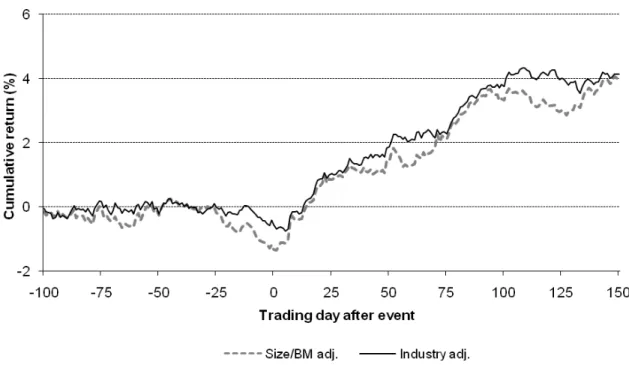
Figure 2 shows average cumulative abnormal returns for 651 events with available data starting from trading day –100 to day 150 after the put sale. To compute daily abnormal returns for each stock, we subtract the daily return on a benchmark portfolio from the corresponding stock return. We use as benchmarks the 49 industry portfolios and 100 size and book-to-market portfolios from Ken French’s website.10 The cumulative return from day –100 to t is then the sum of the daily abnormal returns during that period.

Figure 2 is striking. The average cumulative abnormal return is close to zero during the 100 trading days leading up to the put sale, but increases immediately thereafter. For example, the mean industry-adjusted return is –0.55% on day 0, increases to 1.87% during the first 50 trading days after the sale, and reaches 3.75% by day 100. The cumulative return appears flat during the following 50 days. [INSERT FIGURE 2]

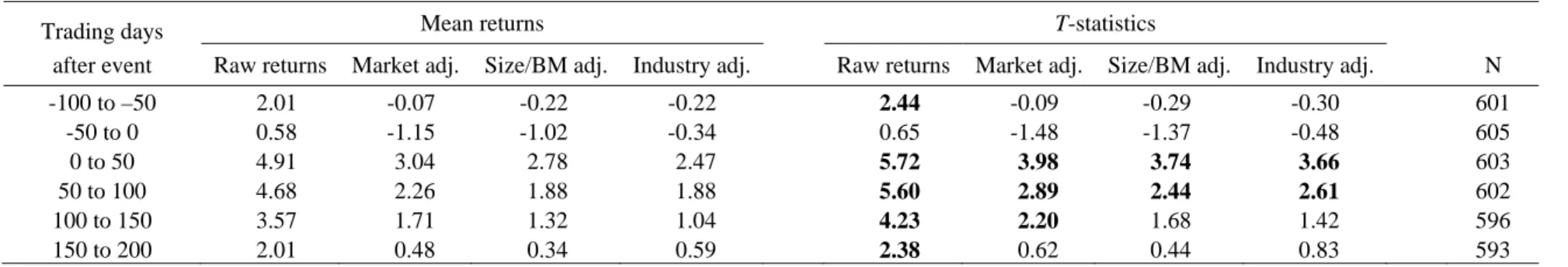
Table III shows that the abnormal post-sale returns are statistically significant. We divide the event horizon into six 50-day intervals: from trading day -100 to -50, from trading day -50 to 0, etc., and report average cumulative returns and t-statistics for each of the 50-day intervals. If a given interval (e.g. -50 to 0) overlaps for different events of the same firm, we keep only the earlier event. Benchmark adjusted returns are positive and statistically significant for the first two intervals following the put sale. The size and book-to-market adjusted return is 2.78% for the first 50 days after the put sale (t-statistic, 3.74), and it is 1.88% for the subsequent 50 days (t -statistic, 2.44). Benchmark adjusted returns are not significant for the two time intervals before the put sale.11 [INSERT TABLE III]

These findings are consistent with the hypothesis that managers use private information to time put option sales. Moreover, managers’ private information is relatively short lived: it affects returns shortly after the event but seems to be fully incorporated into prices within 100 trading days. This is much shorter than the long-run under- or overperformance associated with other corporate events, such as stock issues or open-market share repurchases.12 As we show in Section III.B, most of the post-sale abnormal returns are realized within a short window around the first post-sale earnings announcement, which is consistent with the return pattern in Figure 2.

One concern is that the positive abnormal returns after put option sales might be caused by price manipulation. Market participants suggested to us that issuers might increase open market share repurchases when puts approach maturity in order to inflate stock prices and prevent put option exercises. However, we find no evidence of price support or price manipulation. First, there is no price reversal on average following the post-sale price run-up. The cumulative abnormal returns in Table III are consistently positive for days 150 to 200 after put sales, and we find no negative abnormal returns for subsequent time periods. Second, share repurchases do not increase in quarters in which put options mature, suggesting no attempt to inflate stock prices before expiration dates.

A.2.Robustness tests

The t-statistics in Table III could be overstated because event horizons overlap in time across firms. To address this issue, we use the rolling portfolio approach suggested by Fama (1998). Specifically, for each day in the sample period, we construct a backward-looking portfolio consisting of firms that have an event during the past 70 calendar days (we also look at the 140-day horizon; we choose the calendar-time horizons to match the horizons in Table III). We then

regress the portfolio excess returns on the excess returns on the market portfolio and the Fama and French (1993) size and book-to-market factors, and test whether the regression intercepts (alphas) are different from zero. The tests confirm the results in Table III. The daily alpha obtained using the 70-day equal weighted portfolio is 0.07% (t-statistic, 3.32), and it is 0.05% (t -statistic, 2.93) for the 140-day portfolio. The results for the value weighted portfolios are somewhat stronger with an alpha of 0.09% (t-statistic, 3.33) for the 70-day portfolio, and an alpha of 0.08% (t-statistic, 3.57) for the 140-day portfolio.

Put issuers are required to have a share repurchase program, and several studies document positive abnormal returns following the announcements of repurchase programs (e.g., Ikenberry, Lakonishok, and Vermaelen (1995), Peyer and Vermaelen (2009)). We find that the put sale effect is distinct from the repurchase announcement effect. Specifically, we re-run the tests in Table III using size and book-to-market portfolio benchmarks formed only from firms with share repurchase programs.13 We find that abnormal returns obtained using these modified benchmarks are similar to those reported in Table III. This is consistent with a casual comparison of the results in Table III with those in Payer and Vermaelen. For example, Peyer and Vermaelen find no abnormal returns at the five months horizon for either the largest size quintile or the lowest book-to-market quintile of all Compustat firms, which are the quintiles of most put sellers.

B. Stock price reaction to earnings announcements after put option sales

The positive excess returns after put sales raise the question of what kind of inside information managers have. The literature on share repurchases examines whether managers have information about future changes in profitability at the announcement of a share repurchase

program and finds mixed results. Grullon and Michaely (2004) find no evidence that operating performance improves after repurchase announcements, while Lie (2005) reports some improvement. Both Chan, Ikenberry, and Lee (2004) and Lie (2005) find positive abnormal returns around earnings releases following repurchase announcements.14 If managers use private information about future cash flows when they sell put options, then investors should be positively surprised by earnings announcements following put sales. To test this hypothesis, we examine abnormal stock price reactions around the first, second, and third quarterly earnings ann

0-day window around the first earnings announcement after a put sale

rise. It is unlikely that the post-announcement return merely reflects slow market reaction to ouncement after a sale.

Figure 3 shows the average benchmark adjusted cumulative returns for trading days -40 to 40 around the first earnings announcement after a put sale. Similar to Figure 2, we use 49 industry portfolios and 100 size and book-to-market portfolios as benchmarks. Interestingly, the cumulative returns are almost zero up to 5 days before the announcement and increase sharply during the subsequent 35 trading days. For example, the industry-adjusted return is 0.1% on day -6 and reaches 2.75% on day 30. More than 30% of the abnormal 100-day return documented in Table III occurs during the 1

.15 [INSERT FIGURE 3]

Notably, we do not observe a jump in stock prices on the earnings announcement date. Instead, prices on average increase steadily for several weeks following the announcement. This suggests that managers’ private information is not limited to only quarterly earnings. In fact, the disclosure of put option sales in the quarterly or annual filing following an earnings announcement could itself signal insiders’ optimism to the market, causing the stock price to

earnings news. In the accounting literature, any such post-announcement drift is less likely for large-cap firms; from Table IV, we also find no such effect for quarters 2 and 3.16

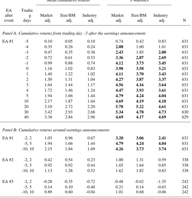
Table IV shows the average cumulative returns and t-statistics for various windows around the first, second, and third earnings announcement after the sale. The bottom panel focuses on 5-day, 11-5-day, and 21-day windows centered at the announcement. Consistent with Figure 3, the cumulative abnormal returns are positive and statistically significant for all three windows around the first announcement. For the second announcement, the returns are still positive but generally not statistically significant. There is no evidence of abnormal returns around the third announcement. [INSERT TABLE IV]

Finally, we examine operating profits before and after put option sales. In particular, we test whether the issuers’ operating performance – measured as return on assets – increased after put sales relative to a sample of control firms with similar pre-sale performance (the details of this analysis are in an online appendix17). We find that this is the case: the issuing firms outperform their benchmarks in the eight quarters following put sales. This evidence is consistent with the positive earnings announcement returns documented above, and it supports the hypothesis that investors were positively surprised by issuers’ operating performance. Overall, the results of this section suggest that managers use both information about future profitability and other inside information to time put sales, and that they do so successfully.

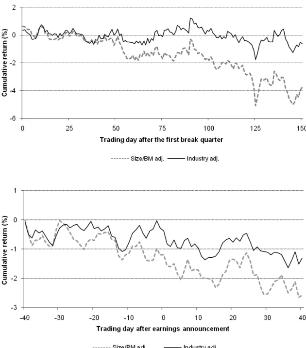
C. Stock price performance during breaks in the put sale programs

If managers use inside information to time put sales, then positive excess returns are more likely to occur subsequent to put issues, and less likely during quarters in which no puts are outstanding. Such a comparison exploits time-series variation in a firm’s put sale intensity, and

also provides a good specification check against the possibility that our models for benchmark returns systematically misprice put issuers throughout the sample period. Put selling firms tend to be large and profitable growth firms, and it is conceivable that this fairly homogeneous group of firms outperformed standard characteristics-based benchmarks during the relevant time period.

Figure 4 shows benchmark adjusted cumulative returns for quarters in which an ongoing put option program is interrupted. We define these “break” quarters as periods in which no options are issued or outstanding, but which are preceded and followed by put option sales. In Figure 4.A, returns are cumulated starting from the end of the first break quarter until the next put sale or until trading day 150. In contrast to the previous findings, there is no evidence of positive excess returns for either industry- or size- and book-to-market adjusted returns. Figure 4.B shows benchmark adjusted cumulative returns around the break quarters’ earnings announcements, and similarly shows no evidence of positive abnormal performance.18 The finding of positive excess returns subsequent to put sales in Figures 2 and 3 and the absence of positive excess returns during break quarters in Figure 4 reinforce the conclusion that managers use inside information to time their put sales. [INSERT FIGURE 4]

D. Do managers time volatility?

The value of a put option increases with the volatility of the underlying stock, so it is possible that managers sell put options when they expect future volatility to be lower than predicted by the market. In this section, we examine volatility changes around put option sales. Finding that volatility declines after puts have been issued would be consistent with volatility timing.

We do not know investors’ actual volatility forecasts. As a proxy, we use realized volatility, and we benchmark volatility and volatility changes against a set of control firms (matched on industry, size, and prior stock return volatility). The comparison to control firms helps reduce noise and control for systematic volatility shifts unrelated to managers’ private information.

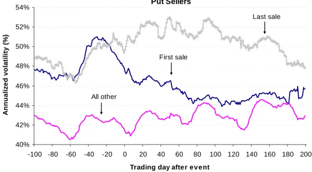
Figure 5 shows volatility levels before and after put issues, and Table V provides formal tests for volatility shifts. We examine separately the first, the last and all other (“intermediate”) issues of a put sale program. We expect that volatility declines are largest when put programs are initiated and smallest, or even reversed, when they are terminated. In Figure 5, volatility is estimated as the annualized standard deviation of daily stock returns over the prior 50 trading days. The top panel shows volatility estimates for put issuers, the bottom panel shows the corresponding estimates for the control firms. To select control firms, we start with all firms from the same Fama-French industry (48 industries) as the put seller and sort them into market capitalization quintiles. We then select the five firms that are closest to the put seller in stock return volatility from the same capitalization quintile. The matching is done at the end of the calendar quarter preceding the put sale. Volatility is measured over the previous six months.

From Figure 5, put issuers’ stock becomes less volatile around the initiation of put sale programs. The issuers’ annualized volatility drops from 50% twenty days prior to the first put sale (day –20) to 46% on day 20, and stays close to this level for the subsequent 180 trading days. In contrast, the control firms’ volatility actually increases slightly, from 50% to 52%, during the same 40-day period.19 This is consistent with volatility timing. There is a slight increase in the issuers’ volatility after intermediate sales, but an even larger increase occurs for the control firms, consistent with some volatility timing also for intermediate sales. Finally, the

sample and control firms show similar volatility changes around final sales, which suggests that managers stop issuing puts when they have no more private information about future volatility. [INSERT FIGURE 5]

Table V presents formal tests of whether the volatility changes around put sales differ between put sellers and control firms. Volatility is estimated as the annualized standard deviation of daily stock returns over 50, 100, and 200 trading days before and after each sale.Panel A shows that, for first sales, the differences between the put sellers’ and the control firms’ volatility changes are highly significant. At the 100-day horizon, average put seller volatility declines by 3.0%, control firm volatility increases by 2.7%, and the 5.7% difference has a t-statistic of 4.8. Similar results obtain for medians. For intermediate sales, it is only at 100-day and 200-day horizons that there is evidence of volatility timing. For these horizons, put issuers’ volatility declines relative to control firms’, and the differences are significant. Finally, there are no significant differences between issuers’ and control firms’ volatility changes around last sales. [INSERT TABLE V]

As a robustness check, Panel B of Table V presents variance ratios, defined as the variance of daily stock returns over 50, 100, and 200 trading days after a put sale divided by the same variance prior to the sale. The message is unchanged: compared to the control firms’, put sellers’ volatilities are unusually low after first and to some extent after intermediate sales (with the latter difference only significant at the 200-day horizon). For first sales, the median 50-day variance ratio is only 0.83 for put sellers compared to 1.09 for control firms. The difference is statistically highly significant.20 Also consistent with Panel A, there are no significant differences between put sellers and controls around final sales. The results of both panels are robust to whether we

examine differences in means, medians, or entire distributions (using a Kolmogorov-Smirnov test), and to whether we aggregate the control firms into a single observation for each put sale.

We conclude that the volatility patterns are consistent with the use of private information about volatility in the timing of put sales. It is important to note, however, that finding a volatility decline after put issues does not necessarily imply that managers consciously monitor and time volatility. Instead, they may simply prefer to issue puts when they perceive the likelihood of major value-relevant news as low, or to sell puts when they believe that put prices are too high, without fully understanding the reason for the overvaluation.

E. Direct evidence on put option outcomes

This section examines the put option outcomes directly. If management has timing ability and can predict either returns or the volatility of returns, then puts issued should have fewer exercises and receive smaller payoffs than would be expected in the absence of private information. Examining put outcomes provides an additional perspective that captures the combined effect of both the high returns and lower volatility after put sales found in Sections III.A and III.D. The option outcome tests are thus potentially better able to detect and illustrate any timing that exists. The results reinforce the paper’s conclusions.

E.1. Measuring abnormal outcomes

To study abnormal put option outcomes, we compare put exercises and payoffs to a benchmark that reflects the outcomes we would expect if management had no private information. We benchmark by matching each put sale with a hypothetical put sale by a control firm selling an equivalent option (e.g., same issue date, maturity, and ratio of stock price to strike

price). Using this pseudo-issuance approach, we then track both the actual and the hypothetical put sale to maturity, and compare the put outcomes. We infer the final outcome for each put by comparing the seller’s stock price at maturity to the strike price. This allows us to include put sales for which the actual outcomes are not reported (349 out of the 802 put sales) and thus avoid concerns about reporting bias. Excluding put sales with unreported outcomes yields qualitatively similar results.

We use two sets of control firms. The first set is the one used in the previous section to test for volatility timing. For each put sale, five control firms are selected based on industry, size, and stock return volatility. Matching on volatility helps assure that the benchmark firms’ shares have similar underlying risk as the sample firms’.21 Controlling for industry and firm characteristics is important because unusual ex-post exercise frequencies and payoffs can be driven by unusual market, industry, or style returns during the sample period, rather than private information. The realized returns of the control firms incorporate this information and permit more precise identification of abnormal exercises and payoffs.

The second set of control firms is chosen based on industry, market-to-book, and firm size. The matching procedure starts with all firms from the same Fama-French industry as the put seller and sorts them into market-to-book quintiles. It then selects the five firms that are closest to the put seller in market capitalization from the same market-to-book quintile. For both sets of control firms, the matching is done at the end of the calendar quarter preceding the put sale date.

E.2.Results

The put outcomes for the sample and the control firms are presented in Table VI. For a substantial number of put sales, the issue dates, strike prices, and maturity dates are not reported

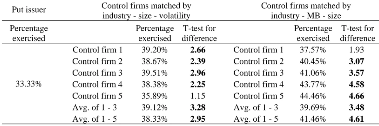
or reported imprecisely. Table VI includes all such cases. We replace the missing data by estimates that correspond to the sample averages reported in Table II. In particular, if a strike price is not reported (n=230 out of 802), we use a strike price that is 5% below the stock price on the put sale date for both the put seller and the control firm. If the maturity date is not reported (n=219 out of 802), we use a time to maturity of 6 months for both firms.22 The results are not sensitive to how we estimate these parameters or whether we exclude cases with missing data. From Table VI, the put sellers have both a significantly lower frequency of put exercises and significantly smaller put payoffs than the control firms. Panel A compares the exercise frequencies. Put sellers experience exercises on 33.3% of the puts they have written. Control firms experience exercises on 38.3% and 41.5% of their puts, depending on the set of control firms chosen. The differences between the groups are highly statistically significant. [INSERT TABLE VI]

Panel B compares the payoffs to put holders. All cases where puts expire out of the money are included, and the dollar payoff at maturity is scaled by the put’s strike price.23 Payouts on puts issued by control firms are fifty percent higher than for actual put sellers: the scaled payoffs on puts written by put sellers average 6.3%, compared to 9.0% and 10.1% for the two sets of control firms. The differences are again highly significant and, together with the results in Panel A, provide further support for the hypothesis that put sellers used private information in the timing of their put sales.

F. The demise of put option sales

Put option sales were at their peak popularity from 1997 to 2000 and rapidly declined over the following three years. By early 2004, put option sales, at least in the form analyzed in this

paper, had essentially vanished. As discussed in Section I.A, there are two likely reasons for the demise of put option sales. First, many issuers lost money in the stock market decline starting in the second half of 2000. This bad experience may have caused managers to question their timing ability. Second, a change in accounting rules in 2003 reduced the attractiveness of put option sales to managers who dislike earnings volatility.

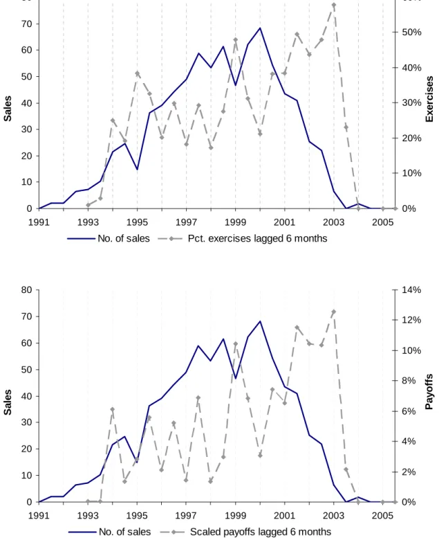
Figure 6 shows the time series of put option sales juxtaposed with the six-months lagged percentage of puts that are exercised and the associated put payoffs from 1991 to 2005. Put sales rose rapidly throughout the 1990s, while put exercises, even though volatile, remained at moderate levels. In the second half of 2000, however, the stock market started to fall. As a result, put exercises and payoffs shot up in the first half of 2001, remained high for the next two years, and reached their highest levels in the last six months of 2002. Over the same time span, put sales fell from 68 sales in the first half of 2000 to 22 sales in the second half of 2002. The financial press, which had given almost uniformly positive coverage to put sales in prior years, turned strongly negative in 2001 and 2002, with Microsoft, Dell, and Electronic Data Systems bearing the brunt of the criticism for their large losses.24 [INSERT FIGURE 6]

Market participants and the practitioner literature suggest that a change in accounting rules introduced in May 2003 may have been a key factor that made put option sales unattractive. FAS No. 150 mandates that outstanding put options be marked to market and changes in their fair value recorded through accounting earnings. Given that put values are a function of stock prices, and stock prices positively correlated with earnings, any put options outstanding after May 2003 are likely to increase earnings volatility. In light of managers’ well-documented aversion to earnings volatility25, it is not surprising that the new accounting rule rendered put sales much

less attractive.26 There were only six put option sales in the first half of 2003, and none in the second half.

IV.Conclusions

The importance of market timing as an explanation for corporate behavior continues to be an unresolved issue. Prior literature on market timing examines equity and debt issues and repurchases. The key problem with these transactions is that each can be motivated by reasons other than mispricing. Put sales, on the other hand, have no obvious motivation other than management’s belief that it can time the market.

We find strong evidence that managers successfully time the market. The stock returns of put issuers outperform their risk-based benchmarks by 4.66% in the 100 trading days after a put sale. Much of the outperformance is realized around and following the first earnings release date after the put sale, suggesting that managers may base their put sale decisions at least partly on private information about future profitability. We also find evidence that managers successfully time the volatility of their stock returns. Realized volatility declines significantly after the first put sale and, relative to control firms, also after intermediate sales.

Our results provide support for the idea that managers can identify mispriced equity and use securities issues to time the market. This is consistent with managers’ self-professed belief in their ability to market time. Our evidence suggests that this belief is based on more than just overconfidence. While our study does not provide direct evidence that market timing is a factor behind equity issues and repurchases, the results here shift our priors on the importance of managerial timing explanations for a broader set of securities transactions.

References

Angel, James J., Gary L. Gastineau, and Clifford J. Weber, 1997, Using exchange traded equity flex put options in corporate stock repurchase programs, Journal of Applied Corporate Finance 10, 109-113.

Atanasov, Vladimir, Stanley B. Gyoshev, Samuel Szewczyk, and George P. Tsetsekos, 2007, Why financial intermediaries buy put options from companies, Working paper, University of Exeter, Exeter, UK.

Baker, Malcolm, Richard S. Ruback, and Jeffrey Wurgler, 2007, Behavioral corporate finance, in Eckbo, B., ed., Handbook of Corporate Finance: Empirical Corporate Finance, Vol. 1 (Handbooks in Finance Series, Elsevier/North Holland).

Ball, Ray, and Philip Brown, 1968, An empirical evaluation of accounting income numbers,

Journal of Accounting Research 6, 159-178.

Bartov, Eli, Suresh Radhakrishnan, and Itzhak Krinsky, 2000, Investor sophistication and patterns in stock returns after earnings announcements, The Accounting Review 75, 43-63.

Bear Stearns Equity Research, 2006, Accounting Issues, January.

Ben-David, Itzhak, John R. Graham, and Campbell R. Harvey, 2007, Managerial overconfidence and corporate policies, Working paper, Duke University, Durham, NC.

Bernard, Victor. L., and Jacob K. Thomas , 1989, Post-earnings-announcement drift: Delayed price response or risk premium? Journal of Accounting Research 27, 1-36.

Bernard, Victor. L., and Jacob K. Thomas, 1990, Evidence that stock prices do not fully reflect the implications of current earnings for future earnings, Journal of Accounting and Economics 13, 305-340.

Bhushan, Ravi, 1994, An informational efficiency perspective on the post-earnings-announcement drift, Journal of Accounting and Economics 18, 45-65.

Brockman, Paul, and Dennis Y. Chung, 2001, Managerial timing and corporate liquidity: Evidence from actual share repurchases, Journal of Financial Economics 61, 417-448.

Brous, Peter A., Vinay Datar, and Omseh Kini, 2001, Is the market optimistic about the future earnings of seasoned equity offering firms? Journal of Financial and Quantitative Analysis 36, 141-168.

Browning, E. S., and Aaron Lucchetti, 1997, More firms use options to gamble on their own stock, Wall Street Journal, May 22, C1.

CBOE Investor Series Paper #2, 2001, Corporate stock repurchase programs and listed options, Chicago Board Options Exchange.

Chan, Konan, David Ikenberry, and Inmoo Lee, 2004, Economic sources of gain in stock repurchases, Journal of Financial and Quantitative Analysis 39, 461-479.

Cornett, Marcia Millon, Hamid Mehran, and Hassan Tehranian, 1998, Are financial markets overly optimistic about the prospects of firms that issue equity? Evidence from voluntary versus involuntary equity issuances by banks, Journal of Finance 53, 2139-2159.

Dann, Larry Y., Ronald W. Masulis, and David Mayers, 1991, Repurchase tender offers and earnings information, Journal of Accounting and Economics 14(3), 217-251.

DeFond, Mark L., and Chul W. Park, 1997, Smoothing income in anticipation of future earnings, Journal of Accounting and Economics 23(2), 115-139.

Denis, David J., and Atulya Sarin, 2001, Is the market surprised by poor earnings realizations following seasoned equity offerings? Journal of Financial and Quantitative Analysis 36, 169-193.

Eckbo, B. Espen, Ronald W. Masulis, and Oyvind Norli, 2007, Security offerings, in Eckbo, B., ed., Handbook of Corporate Finance: Empirical Corporate Finance, Vol. 1 (Handbooks in Finance Series, Elsevier/North Holland).

Fama, Eugene F., 1998, Market efficiency, long-term returns, and behavioral finance,

Journal of Financial Economics 49, 283-306.

Fama, Eugene F., and Kenneth R. French, 1993, Common risk factors in the returns on stocks and bonds, Journal of Financial Economics 33, 3–56.

Fama, Eugene F., and Kenneth R. French, 1997, Industry costs of equity, Journal of Financial Economics 43, 153–194.

Financial Accounting Standards Board, May 2003, Statement of financial accounting standards no. 150.

Foster, George, Chris Olsen, and Terry Shevlin, 1984, Earnings releases, anomalies, and the behavior of securities returns, The Accounting Review 59, 574-603.

Frazzini, Andrea, and Owen Lamont, 2006, The earnings announcement premium and trading volume, Working paper, Yale University.

Gaver, Jennifer J., Kenneth M. Gaver, and Jeffrey R. Austin, 1995, Additional evidence on bonus plans and income management, Journal of Accounting and Economics 19, 3–28.

Gibson, Scott, Paul Povel, and Rajdeep Singh, 2006, The information content of put warrant issues, Working paper, University of Minnesota, Minneapolis, MN

Gong, Guojin, Henock Louis, and Amy X. Sun, 2008, Earnings management and firm performance following open-market repurchases, Journal of Finance 63, 947-986.

Graham, John R., and Campbell R. Harvey, 2001, The theory and practice of corporate finance: evidence from the field, Journal of Financial Economics 60, 187-243.

Grullon, Gustavo, and David L. Ikenberry, 2000, What do we know about stock repurchases,

Journal of Applied Corporate Finance 13, 31-51.

Grullon, Gustavo, and Roni Michaely, 2004, The information content of share repurchase programs, Journal of Finance 59, 651-680.

Gyoshev, Stanley B., 2001, Synthetic repurchase programs through put derivatives: theory and evidence, Ph.D. thesis, Drexel University, Philadelphia, PA

Ikenberry, David, Josef Lakonishok, and Theo Vermaelen, 1995, Market underreaction to open market share repurchases, Journal of Financial Economics 39, 181-208.

Ikenberry, David, Josef Lakonishok, and Theo Vermaelen, 2000, Stock repurchases in Canada: Performance and strategic trading, Journal of Finance 55, 2373-2397.

Investment Dealers’ Digest, 1991, Street pitches put-writing in wake of SEC decision, March 25.

Jenter, Dirk, 2005, Market timing and managerial portfolio decisions, Journal of Finance 60, 1903-1949.

Kothari, S. P., and Jerold B. Warner, 2007, The econometrics of event studies, in Eckbo, B., ed., Handbook of Corporate Finance: Empirical Corporate Finance, Vol. 1 (Handbooks in Finance Series, Elsevier/North Holland).

Laderman, Jeffrey, 1998, Share buybacks that pay back in spades – Hedging techniques are earning millions in tax-free income for savvy companies, Business Week 3566, February 23.

Lakonishok, Josef, and Inmoo Lee, 2001, Are insider trades informative? Review of Financial Studies 14, 79-112.

Lie, Erik, 2005, Operating performance following open market share repurchase announcements, Journal of Accounting and Economics 39, 411-436.

Maffei, Gregory, 1998, The purpose of put warrants, New York Times, Letter to the Editor, December 20.

McDonald, Robert L., 2004, The tax (dis)advantage of a firm issuing options on its own stock, Journal of Public Economics 88, 925-955.

Mitchell, Mark L., and Erik Stafford, 2000, Managerial decisions and long-term stock price performance, Journal of Business 73, 287-329.

Peyer, Urs, and Theo Vermaelen, 2009, The nature and persistence of buyback anomalies,

Review of Financial Studies 22, 1693-1745.

Posell, Jordan, and Kenneth Eades, 1992a, International Business Machines Issuer Put Options, Darden Graduate Business School Foundation, Charlottesville, VA.

Posell, Jordan, and Kenneth Eades, 1992b, International Business Machines Issuer Put Options: Teaching Note, Darden Graduate Business School Foundation, Charlottesville, VA.

Rangan, Srinivasan, 1998, Earnings management and the performance of seasoned equity offerings, Journal of Financial Economics 50, 101-122.

Ronen, Joshua, and Simcha Sadan, 1981, Smoothing income numbers: Objectives, means and implications, Addison-Wesley Publishing Company, Reading, MA.

Salomon Brothers, 1994, Equity put warrants, April.

Shivakumar, Lakshmanan, 2000, Do firms mislead investors by overstating earnings before seasoned equity offerings? Journal of Accounting and Economics 29, 339-371.

Sidel, Robin, Gary McWilliams, and Thomas Burton, 2002, Dell, Eli Lilly join EDS in risky options game, Wall Street Journal, Sept. 27, C1.

Skinner, Douglas J., 1989, Options markets and stock return volatility,

Journal of Financial Economics 23, 61-78.

Spagat, Elliot, and Gary McWilliams, 2002, EDS made losing bet on its stock, Wall Street Journal, Sept. 25, A3.

Taub, Scott A., 2004, Remarks before the 2004 AICPA National Conference on current SEC and PCAOB developments, available at http://www.sec.gov/news/speech/ spch120604sat.htm

Teach, Edward, 1999, Gregory B. Maffei, CFO Magazine, October 1.

0 20 40 60 80 100 120 140 1991 1992 1993 1994 1995 1996 1997 1998 1999 2000 2001 2002 2003 2004 Number of firms Number of put sales

Figure 1. Number of put sales and put issuing firms by year. There are 137 put issuing firms and 802 put sales from 1991-2004. Depending on available data, a put sale represents either an individual transaction or several transactions occurring within one reporting period, usually a fiscal quarter. The precise date of the put sale is in most cases not reported. This figure assumes the transaction occurred on the last day of the “sale period”, usually the fiscal quarter during which the sale must have occurred.

Figure 2. Cumulative abnormal returns around put option sales. The figure shows average benchmark adjusted cumulative returns from trading day –100 to +150 after the put sale event (as defined in Table III). There are 137 put selling firms and 651 put sale events from 1991-2004 with available return data on day – 100. The cumulative return for trading day t is the sum of daily returns from trading day –100 to t. Daily abnormal returns are computed by subtracting the daily return on a benchmark portfolio from the corresponding stock return. We use two benchmarks: the 49 industry portfolios and the 100 size and book-to-market portfolios from Ken French’s website (see Fama and French (1993 and 1997)).

Figure 3. Cumulative abnormal returns around the first earnings announcement after a put option sale. The figure shows average benchmark adjusted cumulative returns from trading day –40 to 40 after the first earnings announcement following a put sale event (as defined in Table III). There are 137 put selling firms and 631 put sale events from 1991-2004 with available announcement and return data. Daily abnormal returns are computed by subtracting the daily return on a benchmark portfolio from the corresponding stock return. We use two benchmarks: the 49 industry portfolios and the 100 size and book-to-market portfolios from Ken French’s website (see Fama and French (1993 and 1997)).

Figure 4. Abnormal returns during breaks in put option programs. The figure shows abnormal returns for quarters in which an ongoing put option program is interrupted and subsequently resumed. These “break” quarters are quarters in which no options are issued or outstanding, but which are preceded and followed by put option sales. In the first panel, returns are cumulated started from the end of the first break quarter until the beginning of the next issue period (or up to trading day 150, whichever comes first). There are 107 quarters (28 firms) with returns available on day one, and 62 quarters with returns available on day 150. The second panel shows cumulative returns around earnings announcements for the 99 break quarters depicted in the first panel for which earnings announcement dates are available. Here, returns are cumulated from day -40 through day +40 after the earnings announcement.

Put Sellers 40% 42% 44% 46% 48% 50% 52% 54% -100 -80 -60 -40 -20 0 20 40 60 80 100 120 140 160 180 200 Trading day after event

A n n u al iz ed vo la ti li ty (% ) All other First sale Last sale Control Firms 40% 42% 44% 46% 48% 50% 52% 54% -100 -80 -60 -40 -20 0 20 40 60 80 100 120 140 160 180 200 Trading day after event

A n nua liz e d v o la tilit y ( % ) All other First sale Last sale

Figure 5. Stock return volatility around put option sales. The figure shows average stock return volatility estimated for rolling windows around the put sale event (as defined in Table III). Volatility on trading day t is the (annualized) standard deviation of daily stock returns from t-50 to t-1. We require that returns are available for 50 trading days for each estimate. The figure shows estimates for windows ending on day –100 to 200 after the put sale event. The first panel shows volatility estimates for put sellers, and the second panel for industry-, size, and volatility-matched control firms. The average volatility is computed separately for the first, last, and all other put option sales in a put sale program. There are 137 first sales, 137 last sales, and 402 intermediate sales with available volatility estimates for day 0.

0 10 20 30 40 50 60 70 80 1991 1993 1995 1997 1999 2001 2003 2005 Sa le s 0% 10% 20% 30% 40% 50% 60% Ex e rc is e s

No. of sales Pct. exercises lagged 6 months

0 10 20 30 40 50 60 70 80 1991 1993 1995 1997 1999 2001 2003 2005 Sa le s 0% 2% 4% 6% 8% 10% 12% 14% Pa y o ff s

No. of sales Scaled payoffs lagged 6 months

Figure 6. Aggregate put sales, lagged exercises, and lagged payoffs from 1991 to 2005. The figure shows the number of put sales, the lagged percentage of puts exercised, and the associated put payoffs for the first and the last half of each calendar year. Put exercises and payoffs are lagged by 6 months. Exercises and payoffs are deduced by comparing the issuer’s stock price to the put’s strike price at maturity. Put payoffs are scaled by the strike price.

Table I

Descriptive statistics for put issuers, repurchasing firms, and all Compustat firms during 1991 to 2004

The samples consist of 137 put issuers (355 firm-years), 5,523 repurchasing firms (13,087 firm-years), and 14,263 Compustat firms (99,546 years). A firm-year is included in the put issuer sample if the firm has at least one put option sale in the fiscal firm-year. A firm-firm-year is included in the repurchaser sample if the firm repurchases shares worth at least 0.5% of the prior-quarter book assets in at least one quarter of the fiscal year. ASSETS and SALES are book assets and sales ($billions). B/M is the ratio of the book value to the market value of common stock. R&D, PPE, and CASH are R&D expense, PP&E plus inventory, and cash plus short-term investments, respectively, all scaled by book assets. R&D and PPE are set to zero if they are missing on Compustat. ROA is operating income after depreciation scaled by book assets. Dividend is a dummy variable equal to one if the firm pays a dividend. Leverage equals total debt divided by the sum of total debt and the book value of common stock. Net repurchase is the difference between the purchase and sale of common and preferred stock scaled by the sum of the market value of common stock and the book value of preferred stock. Some variables are not available for the full samples. All variables are winsorized at the 1st and the 99th percentile in the Compustat sample.

Put issuers Repurchasing firms All Compustat firms

Mean Median Std Mean Median Std Mean Median Std

Assets 10.01 2.58 15.61 2.31 0.26 7.00 2.32 0.18 8.01 Sales 6.06 2.11 7.83 1.83 0.25 4.49 1.19 0.10 3.70 B/M 0.38 0.31 0.30 0.62 0.47 0.54 0.72 0.56 0.65 R&D 0.05 0.02 0.06 0.04 0.00 0.08 0.04 0.00 0.10 PPE 0.40 0.39 0.25 0.37 0.36 0.25 0.36 0.34 0.28 Cash 0.16 0.09 0.18 0.18 0.10 0.21 0.17 0.07 0.22 ROA 0.12 0.12 0.12 0.06 0.10 0.21 -0.01 0.05 0.25 Dividend 0.61 1.00 0.49 0.47 0.00 0.50 0.39 0.00 0.49 Leverage 0.33 0.33 0.26 0.25 0.20 0.24 0.32 0.29 0.27 Net repurchase 0.02 0.02 0.06 0.01 0.02 0.12 -0.04 -0.00 0.12

Table II

Summary statistics for put option sales and programs

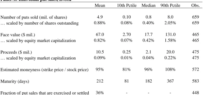
The total number of firms with put sales programs is 137, and the total number of put sales is 802. This excludes 32 maturity extensions of previously sold puts. The number of observations is reduced further because of missing data. The face value of a put issue is the number of puts sold times the average strike price. The estimated moneyness of a put issue is the ratio of the average strike price to the issuer’s stock price on the put sale date. If the sale date is unavailable, we use the average price during the sale period (usually the fiscal quarter of the sale). The maturity of a put issue is the number of days between the put sale date (or the midpoint of the sale period) and the maturity date (or the midpoint of the maturity period). The fraction of all put issues exercised or settled is reported only for issues that can be traced from sale to maturity and for which the final outcome is reported by the issuer.

Panel A: Individual put sales, n=802

Mean 10th Pctile Median 90th Pctile Obs.

Number of puts sold (mil. of shares) 4.9 0.10 0.8 8.0 659

… scaled by number of shares outstanding 0.88% 0.08% 0.40% 2.05% 659

Face value ($ mil.) 67.0 2.70 17.7 131.0 465

… scaled by equity market capitalization 0.82% 0.07% 0.42% 1.58% 465

Proceeds ($ mil.) 10.5 0.25 2.1 20.0 475

… scaled by equity market capitalization 0.09% 0.01% 0.04% 0.22% 475 Estimated moneyness (strike price / stock price) 95% 81% 96% 108% 572

Maturity (days) 212 81 182 367 583

Fraction of put sales that are exercised or settled 36% - - - 448

Panel B: Put sale programs, n=137

Mean 10th Pctile Median 90th Pctile Obs.

Number of put sales 5.9 1 4 13 137

Number of puts sold (mil. of shares) 21.1 0.40 2.7 25.2 108

… scaled by number of shares outstanding 4.15% 0.52% 1.84% 9.37% 108

Face value ($ mil.) 223.4 5.20 43.7 286.0 68

… scaled by equity market capitalization 3.47% 0.56% 1.84% 7.99% 68

Proceeds ($ mil.) 53.4 0.43 5.8 85.1 84

… scaled by equity market capitalization 0.42% 0.03% 0.14% 1.18% 84 Program length (years)

… from the first to the last put sale 2.1 0.08 1.3 5.3 137

… from the first put sale to the last exercise or

expiration 2.8 0.59 2.0 6.3 137

Table III

Abnormal returns around put option sales

The table shows average cumulative returns and t-statistics for various windows around the put sale events. The precise date of a put sale is usually not reported, and we define an event as the last day of the “sale period”, which is usually the fiscal quarter during which the sale takes place. If multiple sales occur during one sale period, we treat these sales as one event. There are 137 put selling firms and 664 put sale events from 1991-2004 with available return data on the event day. Cumulative returns are computed for six 50-day intervals: from trading day –100 to –50, from trading day –50 to 0, etc. If a given interval (e.g. –50 to 0) overlaps for different events of the same firm, we keep only the earlier event. The cumulative return is the sum of daily returns during the 50-day interval. Daily abnormal returns are computed by subtracting the daily return on a benchmark portfolio from the corresponding stock return. We use three benchmarks: the value-weighted

CRSP index, the 49 industry portfolios and the 100 size and book-to-market portfolios from Ken French’s website (see Fama and French (1993 and 1997)). Trading days

after event

Mean returns T-statistics

Raw returns Market adj. Size/BM adj. Industry adj. Raw returns Market adj. Size/BM adj. Industry adj. N

-100 to –50 2.01 -0.07 -0.22 -0.22 2.44 -0.09 -0.29 -0.30 601 -50 to 0 0.58 -1.15 -1.02 -0.34 0.65 -1.48 -1.37 -0.48 605 0 to 50 4.91 3.04 2.78 2.47 5.72 3.98 3.74 3.66 603 50 to 100 4.68 2.26 1.88 1.88 5.60 2.89 2.44 2.61 602 100 to 150 3.57 1.71 1.32 1.04 4.23 2.20 1.68 1.42 596 150 to 200 2.01 0.48 0.34 0.59 2.38 0.62 0.44 0.83 593

Table IV

Abnormal returns around earnings announcements following put option sales

The table shows average cumulative returns and t-statistics around the first three earnings announcements (EA) following a put sale event (as defined in Table III). The sample consists of 137 put selling firms and 631 earnings announcements from 1991-2004. Panel A shows cumulative returns from trading day –5 to 40 after the first announcement; Panel B shows cumulative returns for shorter windows centered around the first, second, and third announcement. In Panel B, the sample of 338 second announcements does not include announcements that are also first announcements for subsequent sales by the same firm. Similarly, the sample of 242 third announcements does not include announcements that are also first or second announcements for later sales. The cumulative return is the sum of daily returns during the event window. Daily abnormal returns are computed by subtracting the daily return on a benchmark portfolio from the corresponding stock return (the benchmarks are described in Table III).

EA after event

Mean cumulative returns T-statistics

Tradin g days Market adj. Size/BM adj. Industry adj. Market adj. Size/BM adj. Industry adj. N

Panel A: Cumulative returns from trading day –5 after the earnings announcement

EA #1 -5 0.10 0.05 0.10 0.74 0.42 0.83 631 -4 0.35 0.26 0.24 2.08 1.60 1.61 631 -3 0.47 0.35 0.36 2.43 1.85 2.00 631 -2 0.72 0.61 0.53 3.36 2.87 2.69 631 -1 0.99 0.88 0.74 4.12 3.73 3.45 631 0 1.16 1.02 0.83 3.98 3.58 3.21 631 1 1.40 1.22 1.02 4.11 3.70 3.43 631 2 1.50 1.31 1.04 4.27 3.87 3.37 631 3 1.64 1.44 1.17 4.56 4.16 3.64 631 4 1.72 1.46 1.24 4.47 3.93 3.61 631 5 1.94 1.66 1.44 4.79 4.24 4.04 631 10 2.17 1.87 1.64 4.69 4.19 4.10 631 20 3.10 2.72 2.20 5.78 5.22 4.61 631 30 3.42 2.93 2.68 5.34 4.78 4.73 630 40 3.36 2.84 2.96 4.69 4.17 4.69 629

Panel B: Cumulative returns around earnings announcements

EA #1 -2, 2 1.03 0.96 0.67 3.20 3.06 2.41 631 -5, 5 1.94 1.66 1.44 4.79 4.24 4.04 631 -10, 10 2.15 1.84 1.69 4.26 3.73 3.74 631 EA #2 -2, 2 0.42 0.54 0.23 1.00 1.31 0.59 338 -5, 5 0.92 0.92 0.44 1.65 1.64 0.85 338 -10, 10 1.13 1.28 0.52 1.62 1.82 0.83 338 EA #3 -2, 2 -0.28 -0.35 -0.72 -0.48 -0.62 -1.35 242 -5, 5 0.14 0.10 -0.40 0.21 0.14 -0.63 242 -10, 10 0.89 0.60 -0.04 1.01 0.68 -0.06 242