Efficient Identification of Additive Link Metrics via Network Tomography

Efficient Identification of Additive Link Metrics via

Network Tomography

Liang Ma

, Ting He

, Kin K. Leung

, Don Towsley

, and Ananthram Swami

∗_{University of Massachusetts, Amherst, MA, USA. Email: [email protected]} §_{Army Research Laboratory, Adelphi, MD, USA. Email: [email protected]}

Abstract—We investigate the problem of identifying individual link metrics in a communication network from accumulated end-to-end metrics over selected measurement paths, under the assumption that link metrics are additive and constant during the measurement, and measurement paths cannot contain cycles. According to linear algebra, all link metrics can be uniquely identified when the number of linearly independent measurement paths equalsn, the number of links. It is, however, inefficient to collect measurements from all possible paths, whose number can grow exponentially inn, as the number of useful measurements (from linearly independent paths) is at mostn. The aim of this paper is to develop efficient algorithms for constructing linearly independent measurement paths and calculating link metrics. We propose one algorithm which can construct nlinearly indepen-dent, cycle-free paths between monitors without examining all candidate paths, whose complexity is quadratic in n. A further benefit of the proposed algorithm is that the generated paths satisfy a nested structure that allows linear-time computation of link metrics without explicitly inverting the measurement matrix. Our evaluations on both synthetic and real networks verify the superior efficiency of the proposed algorithms, which are orders of magnitude faster than benchmark solutions for large networks.

I. INTRODUCTION

Accurate and efficient monitoring of internal network state (e.g., delays and loss rates on internal links) is essential for various network operations such as route selection, resource allocation, and fault diagnosis. Directly measuring the per-formance of individual network elements (e.g., nodes/links) is, however, not always feasible due to the overhead caused by measurement traffic and the lack of support at internal network elements for making such measurements [1]. These limitations motivate the need for external approaches, where we infer the states of internal network elements by measuring the performance along selected paths from a subset of nodes with monitoring capabilities, hereafter referred to asmonitors. Depending on the measurement technique, external approaches can be classified as hop-by-hop approaches or end-to-end approaches. The former rely on special diagnostic tools such astraceroute,pathchar,clink, andpipechar [2] to reveal fine-grained performance metrics of individual links by sending active probes. These tools estimate link-level metrics such as delays, losses, and bandwidths by exchanging Internet

The extended version of this paper has been published inICDCS’13. Research was sponsored by the U.S. Army Research Laboratory and the U.K. Ministry of Defence and was accomplished under Agreement Number W911NF-06-3-0001. The views and conclusions contained in this document are those of the authors and should not be interpreted as representing the official policies, either expressed or implied, of the U.S. Army Research Laboratory, the U.S. Government, the U.K. Ministry of Defence or the U.K. Government. The U.S. and U.K. Governments are authorized to reproduce and distribute reprints for Government purposes notwithstanding any copyright notation hereon.

Control Message Protocol (ICMP) packets with each interme-diate node. Their estimates, however, have known accuracy issues due to asymmetry in routes and different priorities of ICMP and data packets. Some intermediate nodes may even be configured to ignore ICMP packets altogether. Moreover, the measurement process generates a heavy traffic load that competes for valuable network resources with data traffic.

Alternatively, end-to-end approach provides a light-weight solution that only requires the measurement of end-to-end performance metrics (e.g., end-to-end delays) between mon-itors, and uses network tomography techniques to solve for the corresponding metrics at individual links. Generally, network tomography, originated by Vardi [3], refers to the methodology of inferring fine-grained network characteristics from aggregate measurements; in our context, the fine-grained characteristics are individual link metrics, and the aggregate measurements are end-to-end metrics on selected measurement paths1_{. Since only end-to-end measurements are required,}

network tomography can utilize passive measurements from the transmissions of data packets [4], thus reducing traffic overhead as well as avoiding the need for internal cooperation or equal treatment of control/data packets.

A case of particular interest in network tomography is the inference of additivelink metrics, i.e., the end-to-end metric over a path of multiple links is the sum of individual link metrics. A typical example of an additive metric is delay, while a multiplicative metric (e.g., packet delivery ratio) can be expressed in an additive form using the log(·) function. For additive metrics, we can formulate the problem as that of solving a system of linear equations, where the unknown variables are the link metrics, and the known constants are the end-to-end path measurements, each equal to the sum of the corresponding link metrics. The goal of network tomography is essentially to solve this linear system of equations.

Most existing work on network tomography emphasizes inferring as much as possible about link metrics from available path measurements. However, past experience shows that it is frequently impossible to uniquely identify all link metrics from path measurements [5], [6], [7]. In the language of linear algebra, this is because the linear system associated with the measurement paths is noninvertible, i.e., the number oflinearly independentpaths is smaller than the number of links. To make the system invertible, we need to first ensure that there exists a sufficient number of linearly independent paths. To this end, we established in [8] necessary and sufficient conditions on the structure of the network (including the topology and the 1_{The original work [3] addresses a different problem of inferring}

source-destination traffic matrix from aggregate traffic at relay nodes. Both traffic matrix estimation and link metric identification are representative applications of network tomography [4].

placement of monitors) for it to beidentifiable, i.e., the number of linearly independent measurement paths equals the number of links, where measurement paths are restricted to cycle-free paths to conform with the requirement of routing protocols.

However, even if a network is known to be identifiable, it is still a challenge to determine a minimum set of paths to measure. Mathematically, this is because many paths are linearly dependent in that they can be represented as linear combinations of a subset of paths, and hence their measurements do not provide further information about link metrics. In general, the total number of candidate measurement paths in a network with n links can be exponential inn, but only (up to)nof them are linearly independent and thus useful for link identification. A smart strategy for finding nlinearly independent paths will not only save resources in collecting measurements, but also increase the efficiency of calculating link metrics by discarding redundant linear equations.

In this paper, we investigate the following closely-related problems in network tomography: (a) Given an arbitrary identifiable network G withnlinks (verified by the condition derived in [8]), how can we efficiently construct n linearly independent, cycle-free paths between monitors? (b) Given measurements on the constructed paths, how can we efficiently calculate individual link metrics? The emphases in both prob-lems are onefficiency; although one can enumerate all possible paths until findingnlinearly independent ones, such a method will incur a large cost (exponential inn) and is thus unsuitable for large networks. In both problems, we assume that the link metrics are additive and constant. Note that a “constant” link metric refers to one that either changes slowly relative to the measurement process, or that is a statistical characteristic (e.g., mean, variance) of the link that stays constant over time2_.

A. Related Work

Based on the model of link metrics, existing work on network tomography can be broadly classified as algebraic and statistical approaches. Algebraic approaches, as in this paper, model link metrics as unknown constants, and use techniques from linear algebra to compute link metrics from path metrics [5], [6]. Statistical approaches model link metrics as random variables with (partially) unknown probability distributions, and apply various parametric/nonparametric techniques to estimate the distributions from realizations of path metrics [9], [1], [10].

When all nodes are allowed to participate in the measure-ment process, multicast can be exploited as a measuremeasure-ment method with broad coverage and low overhead [11], [12]. Sub-trees and unicast are employed in [4], [13] as alternatives with more flexibility in selecting receivers, but measurements are still conducted along multicast trees.

When only selected nodes (i.e., monitors) can participate in the measurement process, as assumed in this paper, the problem becomes more challenging. When all but k link metrics are zero, [14] propose schemes inspired by compressive sensing to construct measurement paths to identify theknon-zero link metrics. For arbitrary valued link metrics, few positive results are known. If the network is directed (links have different metrics in different directions), [10] proves that not all link metrics are identifiable unless every non-isolated node is a monitor, and [5] shows that even if every node is a monitor, unique link identification is 2_{In this case, end-to-end measurements are also statistical characteristics,}

e.g., path mean/variance. In the case of variance, we also need the indepen-dence between link qualities to make the metric additive.

still impossible if measurements are restricted to cycles. If the network is undirected (links have equal metrics in both directions), [15] proposes an efficient algorithm to identify link metrics, given that monitors can measure cycles or paths containing cycles. A similar study in [16] characterizes the minimum number of measurements needed to identify a broader set of link metrics (including both additive and nonadditive metrics), under the stronger assumption that measurement paths can contain repeated links. Since routing along cycles is typically prohibited by routing protocols, it remains open what the solution becomes if only cycle-free paths can be measured. Given measurements on n linearly independent paths (nis the number of links), a general solution for computing link metrics using classic linear system solvers (e.g. Gaussian elimination with pivoting) takes O(n3_{) time} [17], which can be slow for large n. In this paper, we overcome this drawback by developing efficient algorithms for path construction and link identification in arbitrary identifiable networks, employing only cycle-free paths. B. Summary of Contributions

Our contributions are three-fold:

1)We develop an efficient algorithm to constructnlinearly independent, cycle-free paths between monitors in an arbitrary identifiable network inO(mn)time (mis the number of nodes and n the number of links), significantly improving on the exponential complexity of brute-force methods. The algorithm exploits the existence of three independent spanning trees, a special property of identifiable networks derived from the identifiability condition in [8] (see Theorem III.1).

2)Given measurements along the constructed paths, we de-velop an algorithm to calculate thenlink metrics inO(m+n)

time, improving on the O(n3_{) complexity of the existing} solution [17]. The algorithm exploits a nested structure of the constructed paths to avoid the need to explicitly invert the measurement matrix.

3)We compare the proposed algorithms against benchmark solutions through simulations on both synthetic networks and real ISP networks. The results verify the superior efficiency of the proposed algorithms, which can be more than 100 times faster than the benchmarks for large networks.

We note that not all link characteristics can be modeled as additive metrics (e.g., bit error rates). Our goal in this paper is to uniquely and efficiently identify additive link metrics; studies for non-additive metrics are left to future work.

The rest of the paper is organized as follows. Section II formulates the problem. Section III summarizes the theoretical foundations for developing algorithms. Section IV presents our algorithms for path construction and link identification. Evaluations of the proposed algorithms are given in Section V. Finally, Section VI concludes the paper.

II. PROBLEMFORMULATION

A. Models and Assumptions

We assume that the network topology is known and model it as an undirected graphG= (V, L), whereV andLare the sets of nodes and links, respectively. Without loss of generality, we assumeGis connected, as different connected components have to be monitored separately. Letm:=|V|be the number of nodes andn:=|L|be the number of links inG. Each link li ∈ L (i = 1, . . . , n) is associated with an unknown metric wl_i that represents the average performance (e.g., average delay) of this link, modeled as a constant. In this paper, we assume that link metrics are symmetric in both directions,

TABLE I MAINNOTATIONS Symbol Meaning

V(G),L(G) set of nodes/links in graphG m,n number of nodes/links inG

G+l add a link:G+l = (V(G), L(G)∪ {l}), where the end-points of linklare inV(G)

G ∪ G′ graph union:G ∪ G′= (V(G)∪V(G′), L(G)∪L(G′))

P simple path, defined as a graph with{v0, . . . , vk}andL(P) ={v0v1, v1v2, . . . , vV(kP−)1vk=},

wherev0, . . . , vkare distinct nodes µi µi∈V(G)is thei-th monitor inG wl,cP metric of linkl, sum metric of pathP

i.e., if ij denotes the link from node i to node j, then links ij andjihave the same metric. Table I summarizes the main notation used in this paper (following the convention of [18]). Certain nodes inV are monitors, which can initiate/collecte measurements. We assume source routing at the monitors, i.e., they can control the routing of measurement packets as long as the path begins and ends at distinct monitors and does not contain repeated nodes. In the language of graph theory, we limit measurements to simple paths between monitors. Let w = (wl₁, . . . , wl_n)T denote the column vector of all link metrics, and c = (c_P1, . . . , c_Pγ)T _{the column vector of} all available path measurements, where γ is the number of measurement paths and c_Pi is the sum of link metrics along measurement path Pi. The measurements are linked to the unknown link metrics by the following linear system:

Rw=c, (1)

whereR= (Rij)is a γ×n measurement matrix, with each entryRij ∈ {0,1}indicating whether linkj is on pathi. The network tomography problem is to invert this linear system to solve for wgivenRandc.

A link is identifiable if the associated link metric can be uniquely determined from path measurements; network G is identifiable if all links inGare identifiable. The linear system model (1) implies that to uniquely determine w,Rmust have full column rank, i.e., rank(R) =n. In other words, we must find n linearly independent simple paths between monitors to take measurements. This is highly nontrivial because: (i) there may not exist nlinearly independent simple paths in an arbitrary network with arbitrarily placed monitors; (ii) even if there exists a set of n linearly independent simple paths (not necessarily unique), it remains a challenge to efficiently discover such a set, as the total number of paths can grow exponentially with n. The naive solution of taking measure-ments alongnarbitrarily selected paths is unlikely to uniquely identify all link metrics; an alternative solution of enumerating all possible paths until findingn linearly independent ones is unlikely to scale to large networks due to its exponentially growing complexity in n. It is therefore desirable to have a method that achieves both full rank and efficiency.

B. Objective

Given an identifiable networkG withκ(κ≥3) monitors3_,

the objective of this paper is to develop efficient algorithms for constructing monitor-to-monitor measurement paths and calculating each link metric in G.

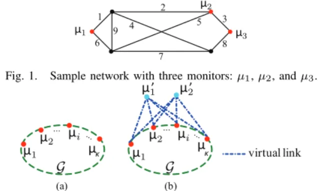
C. Illustrative Example

Fig. 1 displays a sample network with three monitors (µ1– µ3) and nine links (link1–9). To identify all link metrics, nine 3_{Identifiability can be guaranteed by deploying monitors according to the}

Minimum Monitor Placement algorithm in [8].

1 2 3 4 5 6 8 7 9 μ1 μ2 μ3

Fig. 1. Sample network with three monitors:µ1,µ2, andµ3.

(a) (b) ... ... ... ... μ₁μ2 μi μ₁ μ₂ μi κ μ μ₁’ G G virtual link κ μ μ₂’

Fig. 2. (a)Gwithκ(κ≥3) monitors; (b)Gexwith two virtual monitors.

measurement paths are constructed to form the measurement matrixR: µ1→µ2:6 5 6 9 2 1 4 7 5 µ1→µ3:1 4 8 6 7 8 6 9 4 8 µ2→µ3:3 5 7 8 2 4 8 VR=           0 0 0 0 1 1 0 0 0 0 1 0 0 0 1 0 0 1 1 0 0 1 1 0 1 0 0 1 0 0 1 0 0 0 1 0 0 0 0 0 0 1 1 1 0 0 0 0 1 0 1 0 1 1 0 0 1 0 0 0 0 0 0 0 0 0 0 1 0 1 1 0 0 1 0 1 0 0 0 1 0           ,

whereRij = 1if and only if link j is on path i. Given the vector c of sum metrics measured on the constructed paths, we have a linear system Rw = c. Since R is invertible in this example, we can uniquely identify w by w =R−1c. If path65(first row inR) is replaced by path12, then the new measurement matrix is not invertible, and thus cannot uniquely identify all link metrics. A careful selection of measurement paths is therefore crucial.

III. FUNDAMENTALS ONNETWORKIDENTIFIABILITY

A. Conditions for Identifiability

A prerequisite of any successful link identification method is that the network contain a sufficient number of linearly independent measurement paths. In our previous work [8], we translated this requirement into explicit conditions on the net-work topology and the placement of monitors as stated below.

Theorem III.1 ([8]). Given κ(κ≥2) monitors deployed to measure simple paths between monitors, we have that:

1) ifκ= 2, then no nontrivialG(withn >1) is identifiable regardless of its topology and the placement of monitors; 2) ifκ≥3, thenGis identifiable if and only if the associated extended graphGex (see Fig. 2) is 3-vertex-connected. The extended graphGex is constructed as follows: as illus-trated in Fig. 2, given a networkG with monitorsµ1,· · ·, µκ, Gexis obtained by adding twovirtual monitorsµ′₁andµ′₂, and

2κvirtual links between each pair of virtual-actual monitors. The theorem states that the sufficient and necessary condition for identifying all link metrics inG is that there are at least

3 monitors, and the extended graph remains connected after removing two arbitrary nodes (i.e., it is3-vertex-connected). B. Test and Assurance of Identifiability

Besides being of theoretical value, the above result also has direct application to algorithm design. A straightforward application leads to an algorithm that tests the identifiability of a given networkGunder a given monitor placement. This is achieved by applying a classic algorithm [19] to test3 -vertex-connectivity of Gex, with a complexity of only O(m+n).

... _... μ₁ μ2 μi μκ G r μ₁’ μ2’ virtual link

Fig. 3. Ther-extended graphG∗exofG.

v μ1 μi κ μ S1 G r u μ2 S2 S₃

Fig. 4. Three internally vertex disjoint paths betweenvandrimply three monitor-to-monitor simple paths:S1∪ S2,S1∪ S3, andS2∪ S3.

A more advanced application is in monitor placement, where the objective is to achieve network identifiability with the minimum number of monitors. The algorithm, calledMinimum Monitor Placement (MMP), decomposes G into subgraphs with certain properties (triconnected components) and sequen-tially places monitors in each subgraph to satisfy the condition in Theorem III.1.2; see [8] for details. MMP is provably optimal in that it minimizes the number of monitors required to guarantee network identifiability. It is also efficient, with a complexity ofO(m+n).

IV. ALGORITHMDESIGN

After verifying that the network is identifiable, i.e., there exist n linearly independent simple paths between monitors, the natural followup questions are: how can we efficiently find nsuch paths, and how can we efficiently compute link metrics from measurements on these paths? In this section, we first provide the key idea behind our solutions and then formally present the algorithms and analyze their complexity.

The idea of efficient path construction and link identification originates from the identifiability condition in Theorem III.1.2. Since the condition is necessary, any identifiable network G must have a 3-vertex-connected extended graph Gex. We further extend Gex by adding another virtual node r and connecting it to the virtual monitorsµ′₁, µ′₂and any one of the real monitors µi (for any i ∈ {1, . . . , κ}) with three virtual links, as illustrated in Fig. 3; we refer to the new graph as the r-extended graph, denoted by G∗ex. It can be shown that G∗

ex is also 3-vertex-connected. By Menger’s theorem [18], this implies that there exist at least3internally vertex disjoint simple paths between any two nodes in G_ex∗ (i.e., the paths are disjoint except at end-points). In particular, as illustrated in Fig. 4, each non-monitor node v has (at least)3 internally vertex disjoint simple paths to the virtual node r. Since any path to rmust go through at least one (real) monitor, we can truncate each path at the first monitor on the way to r (i.e., removing the sub-path from this monitor tor), which provides threev-to-monitor pathsS1,S2,andS3that are disjoint except atv. This allows us to construct three monitor-to-monitor paths P1 := S1∪ S2, P2 := S1∪ S3, and P3 := S2∪ S3, each being a simple path valid for taking measurements. Based on measurementsc_Pi (i= 1,2,3) from the constructed paths, we can obtain the individual metrics ofSiby solving the following linear equations:

{ _c

S1+cS2 =cP1,

c_S1+c_S3 =c_P2, c_S2+c_S3 =c_P3,

Algorithm 1: Spanning Tree-based Path Construction (STPC)

input : NetworkG withκmonitors such that every link inG is identifiable

output: Measurement paths in the form of (rows in) a measurement matrixR

1 R=∅;

2 ConstructG_ex∗ fromG; //see Fig. 3

3 Find three spanning treesT1,T2 andT3 ofGex∗ that are

pairwise independent wrtr by the algorithm in [20]; 4 foreachnodevinG do 5 ifvis a monitorthen 6 Pv1← Sv1;Pv2← Sv2;Pv3← Sv3; 7 else 8 Pv1← Sv1∪ Sv2;Pv2← Sv2∪ Sv3; Pv3 ← Sv3∪ Sv1; 9 end

10 Append all non-degeneratePvi (i= 1,2,3) toR;

11 end

12 foreachlinklnot inT1∪ T2∪ T3 do

13 Find a simple monitor-to-monitor pathPltraversinglin

graphT1∪ T2∪ T3+l(see Algorithm 2);

14 AppendPltoR;

15 end

where c_Si (i = 1,2,3) is the path metric on Si. Repeating this procedure for every node in G yields the metrics from each node to three monitors. Furthermore, we will show a way to construct these paths such that they are nested, i.e., if a path from v to monitor µ2 goes through a neighbor u, as illustrated in Fig. 4, thenumust use the same path to connect to µ2. Therefore, we can calculate the metric of link uv by subtracting the u → µ2 path metric from the v → µ2 path metric. We now present the algorithms in detail.

A. Spanning Tree-based Path Construction

Given an arbitrary network G, we propose an algorithm, Spanning Tree-based Path Construction (STPC), to construct linearly independent monitor-to-monitor paths, so that links can be uniquely identified from measurements on these paths. We assume that G is identifiable. This is guaranteed by de-ploying monitors according to algorithm MMP in [8], although STPC can also work with other monitor placements as long as network identifiability is guaranteed. In essence, STPC ex-ploits a property of identifiable networks in terms of spanning trees. To this end, we introduce the following definition.

Definition 1. Two spanning trees of an undirected graph G(V, L)areindependent with respect to (wrt) a vertexr∈V if the paths fromv toralong these trees are internally vertex disjoint for every vertex v∈V (v̸=r).

For a 3-vertex-connected graph and any given vertex, Theo-rem 6 in [20] states that there exist three spanning trees that are pairwise independent wrt this vertex. In particular, since the r-extended graph Gex∗ is guaranteed to be 3-vertex-connected for any identifiable network, we will always be able to find three spanning trees ofG_ex∗ that are pairwise independent wrt r. These spanning trees provide three internally vertex disjoint paths from each non-monitor node v to r. As previously illustrated in Fig. 4, STPC constructs measurement paths by truncating these node-to-rpaths at monitors and then concate-nating each pair of truncated paths to form a simple monitor-to-monitor path in the original graph G. See Algorithm 1 for details.

Specifically, STPC has two main steps: (1) constructing measurement paths based on independent spanning trees, and (2) constructing additional paths to measure links not in any

v r w e₂₁ e₂₂ e₁₁ e₃ v r(=u) w e₂ e₁ e₃ (a) u= r (b) u= r μa μb u e₁₂ /

Fig. 5. Constructing measurement path traversing a non-tree linkvw. Algorithm 2: Path Construction for Non-Tree Links

input : TreesT1,T2,T3 constructed in Algorithm 1 and a link

l=vwnot in the trees

output: A simple monitor-to-monitor pathPl traversingland

links in the trees

1 From the trees, find two pathsve2rand ve3r fromvtorthat

do not traversew, and a pathwe1r fromwto rthat does not

traversev;

2 On pathwe1rstarting fromw, find the first intersection nodeu

with eitherve2r orve3r; 3 ifu=rthen 4 Pl← Sve2r∪l∪ Swe1r; 5 else 6 Pl← Sve3r∪l∪ Swe11ue22r; 7 end

of the trees. The first step begins with the application of the algorithm in [20] to find three spanning trees Ti (i= 1,2,3) of Gex∗ that are independent wrt r (line 3). Based on these spanning trees, STPC constructs paths to measure links in the trees (lines 4-11). Let Svi (i= 1,2,3) denote a simple path from nodevto the first monitorµ(µ̸=v) towardrinTi. If no suchµexists, thenSvirepresents a degenerate path containing just a single node v. STPC iterates among all nodes inG: if v is a monitor, then Svi (i= 1,2,3) are already monitor-to-monitor simple paths (line 6); ifv is not a monitor, then pairs of Svi’s again form monitor-to-monitor simple paths, asSv1, Sv2, and Sv3 are disjoint except atv (line 8). Therefore, all the constructed pathsPvi(i= 1,2,3) that are non-degenerate (i.e., containing at least one link) are valid measurement paths, and are thus added to the measurement matrix (line 10).

The second step constructs paths for links not in any of the three trees (lines 12-15). For a non-tree link l, i.e., l not in any Ti (i = 1,2,3), STPC invokes an auxiliary algorithm, Algorithm 2, to construct a measurement path Pl through l such that all the other links on this path belong to the trees. Algorithm 2 utilizes a simple observation as follows. As illustrated in Fig. 5, among the three internally vertex disjoint paths from v to r along the three spanning trees, there exist at least two paths, say ve2r and ve3r, that do not traverse w; similarly, there exists at least one path from w to r, say we1r, that does not traverse v (line 1). Starting from w, we follow we1runtil the first intersection uwith either ve2r or ve3r (line 2). Ifu=r as in Fig. 5 (a), then we1r andve2r (or ve3r) are disjoint except at r. Truncating these paths at the first monitors toward rprovides two disjoint paths,Swe₁r andSve₂r, that connectwandvto monitors. Connecting these paths by link vw gives a simple path between monitors that traverses only vwand links in the trees (line 4). Ifu̸=r, we assume without loss of generality that u is an internal node on ve2r as illustrated in Fig. 5 (b), which divides pathwe1r into sub-paths we11u and ue12r, and ve2r into ve21u and ue22r. The new path formed by we11ue22r is disjoint with ve3rexcept atr. Truncating pathswe11ue22randve3ragain provides two disjoint pathsSwe₁₁ue22randSve3rconnectingw

andv to monitors, which together with linkvw form a simple monitor-to-monitor path traversing only vw and links in the trees (line 6). The validity of the algorithm is guaranteed by

the following lemma.

Lemma IV.1. PathPlconstructed by Algorithm 2 is a simple monitor-to-monitor path traversing onlyland links in the trees. Proof:It is easy to see thatPlcontains only one non-tree link, linkl. To verify it as a simple path, it suffices to show that the following paths are disjoint except atr:ve2randwe1rif u=r, orve3randwe11ue22rifu̸=r. The former is trivially satisfied. For the latter, note that sub-path we11u is disjoint withve3rasuis the first intersection (andve3rcannot contain u since it is internally vertex disjoint with ve2r). Moreover, sub-path ue22r is disjoint with ve3r except atr as ve2r and ve3rare internally vertex disjoint. Thus, pathswe11ue22rand ve3r are disjoint except atr, completing the proof.

The correctness of STPC, i.e., the constructed measurement matrixRhas rank n, will be clear in Section IV-B when we present an algorithm to explicitly compute all link metrics from measurements on these paths. In general, further processing is needed to findnlinearly independent rows inR that specify the final set of measurement paths, since Rmay contain superfluous paths. However, we have a stronger result showing that the final processing is as simple as eliminating duplicate paths because all distinct paths (paths that differ in at least one node) found by STPC are linearly independent.

Theorem IV.2. The number of distinct paths constructed by STPC equalsn, the number of links inG.

The proof of Theorem IV.2 is in [21]. Since only distinct paths can be linearly independent, and the number of linearly independent paths constructed by STPC equals n (as these paths can uniquely identify thenlinks; see Section IV-B), The-orem IV.2 implies that all distinct paths found by STPC are lin-early independent. Removing duplicate rows in the constructed Rthus generates ann×n invertible measurement matrix. B. Spanning Tree-based Link Identification

Given the paths constructed by STPC, we are now ready to take measurements and compute link metrics. A straightfor-ward approach is to invert the measurement matrix to solve for the link metrics byw=R−1_{c(assumingRis invertible)}4_,

with a complexity ofO(n3_{), which we seek to avoid. We will} show that the R generated by STPC has a special structure that allows us to directly compute link metrics at a much lower complexity. The algorithm, Spanning Tree-based Link Identification (STLI), consists of three main steps as shown in Algorithm 3: (1) computing node-to-monitor path metrics (lines 1-3), (2) identifying links in the spanning trees (lines 4-12), and (3) identifying the other links (lines 13-15). In the sequel, we use c_P to denote both measured path metric ifP is a monitor-to-monitor path, and calculated path metric ifP is a node-to-monitor path (although the input vector c only contains measured path metrics).

The first step of STLI aims at computing the node-to-monitor metric c_Svi for every node v ∈ V and every i ∈

{1,2,3} (lines 1-3). From the path construction in steps 6 and 8 of STPC, we see that c_Svi is directly measured ifv is a monitor. Ifvis not a monitor, we can construct three linear equations based on measurements onPvi (i= 1,2,3):

   c_Sv1+c_Sv2 =c_Pv1, c_Sv2+c_Sv3 =c_Pv2, c_Sv3+c_Sv1 =c_Pv3, (2)

4_{Existing algorithms, e.g., Gaussian elimination [17], can directly solve for}

Algorithm 3: Spanning Tree-based Link Identification (STLI)

input : Measurement paths and spanning treesTi(i= 1,2,3)

constructed by Algorithm 1, measurementscon the paths

output: Vectorwof link metrics inG 1 foreachnodevinGdo

2 Computec_Svi from measurementsc_Pvi (i= 1,2,3) by (2);

3 end

4 foreachtreeTi(i= 1,2,3)do

5 foreachlinkvwin treeTi(vis closer tor)do

6 ifvis a monitor then 7 wvw=cSwi; 8 else 9 wvw=cSwi−cSvi; 10 end 11 end 12 end

13 foreachlinklnot inT1∪ T2∪ T3 do

14 Computewlby subtracting metrics of the other links onPl

fromc_Pl;

15 end

from which we can compute c_Svi (i= 1,2,3).

The second step aims at solving for metrics of all links in the trees (lines 4-12). Consider a linkvwin treeTi(i∈ {1,2,3}), wherevis one hop closer tor. Ifvis a monitor, then the node-to-monitor path Swi will only contain link vw, and thus its metric is also the metric ofvw (line 7). Ifv is not a monitor, then the node-to-monitor pathSvi must be a sub-path ofSwi, shorter by just linkvw, and thus the difference in their metrics equals the metric ofvw (line 9).

The final step addresses links not in the trees (lines 13-15). Since the measurement path Pl for each non-tree linkl only containsland links in the trees (Lemma IV.1), we just need to subtract from c_Pl the metrics of these tree links as identified in the second step to compute the metric of l (line 14).

Besides computing link metrics, STLI also serves as a constructive proof that the paths constructed by STPC can uniquely identify all links, i.e., the generated Rhas rankn. C. Complexity Analysis

We now analyze the complexity of the proposed algorithms. STPC has an overall complexity of O(mn). Specifically, the complexity of spanning tree construction in line 3 is O(m|L(G_ex∗ )|) [20], which is O(mn) since |L(G_ex∗ )| = O(|L(G)|) =O(n). For lines 4-11, pathsPvi(i= 1,2,3) can be constructed in O(m) time for each nodev; thus, lines 4-11 takeO(m2)time. Finally, lines 12-15 invoke Algorithm 2 O(n)times, and each invocation takes timeO(m). Combining the above yields an overall complexity of O(nm). We point out that it is possible to save some computation by removing redundant links in Gex∗ using anO(m+n)-time algorithm in Section 4 of [20], which reduces the number of links toO(m)

while maintaining the 3-vertex-connectivity. This step reduces the complexity of spanning tree construction to O(m2), but the overall complexity remains the same.

Given measurements on the constructed paths, STLI can compute link metrics in O(m+n) time. Specifically, computingc_Svi (lines 1-3) takesO(m)time. Then computing the metric of each link in the spanning trees (lines 6-10) takes only constant time, and there are O(m) links in the trees, making the complexity of lines 4-12O(m). Finally, computing the metrics of non-tree links (lines 13-15) takesO(n)time as explained below. Thus, the overall complexity is O(m+n).

At first sight, it may seem that line 14 takesO(m)time as there are O(m) link metrics to subtract, making the overall

complexity of STLI O(nm). However, we observe that this step can be implemented in constant time using the knowledge of c_Svi as follows. Consider the two cases in constructingPl as illustrated in Fig. 5. Suppose that pathwe1rbelongs to tree Ti1,ve2rtoTi2, andve3rtoTi3(i1, i2, i3∈ {1,2,3}, i2̸=i3).

In case Fig. 5 (a), the measurement pathPlis a concatenation of link l, path Svi₂, and path Swi₁, and thus the metric of linkl can be computed bywl=c_Pl−c_Svi₂−cSwi₁. In case

Fig. 5 (b), if the first monitor along pathwe11ue22r appears before or atu(e.g.,µa), thenPlconsists ofl,Svi₃, andSwi₁, and thuswl=c_Pl−c_Svi₃−cSwi₁; if the first monitor appears

afteru(e.g.,µb), thenPlconsists ofl,Svi₃,we11u, andSui₂, and thus wl = cPl−cSvi3 −(cSwi1 −cSui1)−cSui2 (since

the metric ofwe11uequalscSwi₁−cSui₁). In all the cases,wl

can be computed in constant time.

The above complexity results are well aligned with needs in practice. Path construction only needs to be performed once for a given topology, and thus can tolerate a higher complexity. In contrast, link identification needs to be performed more fre-quently to keep monitoring the health of links. In this regard, STLI in conjunction with STPC enables fast identification of link metrics that can scale to large networks.

V. PERFORMANCEEVALUATION

To evaluate the performance of STPC and STLI, we conduct a set of simulations on both randomly-generated and real network topologies. Given a network topology, we first apply the optimal monitor placement algorithm MMP in [8] to select a subset of nodes as monitors so that the network is guaranteed to be identifiable. We then apply the proposed algorithms to construct measurement paths between the placed monitors and compute link metrics from measurements on these paths. The focus of our evaluations is on the efficiency, measured by the average running time, of the proposed algorithms in comparison to benchmarks. For path construction, we also evaluate the cost of measuring the constructed paths, in terms of average path length (i.e., number of hops).

As a benchmark for STPC, we use the following algorithm5_,

referred to asRandom Walk-based Path Construction (RWPC). Given an identifiable networkG, RWPC repeats the following steps until the rank of the constructed measurement matrixR equalsn (starting fromR=∅):

(i) starting from a randomly selected monitor, follow a random walker until it hits another monitor;

(ii) remove cycles from the path taken by the random walker to generate a simple monitor-to-monitor path;

(iii) if the generated path is linearly independent wrt existing paths inR, append it toR; otherwise, discard the path. RWPC is essentially a randomized algorithm that examines one path at each iteration until n linearly independent paths are found. In practice, RWPC may iterate indefinitely for large networks. To control its running time, we impose amaximum number of iterationsIMAX, and force RWPC to terminate after IMAXiterations. Consequently, we also measure itssuccess rate r_succ, defined as the fraction of Monte Carlo runs during which RWPC successfully findsn linearly independent paths withinIMAXiterations (the success rate of STPC is always one).

Limiting the number of iterations leads to underestimating the actual running time of RWPC in constructing n linearly 5_{Existing path-construction solutions cannot be used as benchmarks since}

they are not comparable to STPC for these two reasons: (i) most solutions assume given routing rather than controlled routing as assumed in this paper, (ii) even under controlled routing assumption, existing path construction algorithms may contain cycles, which is prohibited in this paper.

independent paths, but it allows us to apply the algorithm to large networks.

As a benchmark for STLI, we use the general solution [4] of inverting the measurement matrix: w=R−1_{c, referred to} as Matrix Inversion-based Link Identification (MILI). HereR is an invertible matrix computed by RWPC if it is successful, or STPC otherwise.

Our simulation results include the following metrics: (a) κ,κ: minimum number of monitors selected by MMP and

its average (for randomly generated topologies); (b) rsucc: success rate of RWPC;

(c) Υ: rank(R)/n for RWPC when it is unsuccessful; (d) tSTPC, tRWPC: average running times of STPC and RWPC;

(e) tSTLI, tMILI: average running times of STLI and MILI;

(f) hSTPC, hRWPC: average lengths of thenpaths constructed by

STPC and RWPC (when successful).

The simulation is implemented in Matlab R2010a and performed on a computer with Intel Core i5-2540M CPU @

2.60GHz, 4.00 GB memory, and 64-bit Win7 OS. A. Random Topologies

We first evaluate the proposed algorithms on synthetic topologies generated according to three different random graph models: Erd¨os-R´enyi (ER) graphs, Random geometric (RG) graphs, and Barab´asi-Albert (BA) graphs. For each model, we fix the number of nodes to 150, and randomly generate 100

graph realizations6, which are then fed to the path construction algorithms. For each generated link, we randomly generate a link metric between 0 and1, which is then used to compute path metrics. Here IMAX is set to 3×n. We now explain the

models and the corresponding results separately.

1) Erd¨os-R´enyi (ER) graph: The ER graph is a simple random graph generated by independently connecting each pair of nodes by a link with a fixed probabilityp. The result is a purely random topology where all graphs with an equal number of links are equally likely to be selected. It is known [22] thatp0= logm/mis a sharp threshold for the graph to be connected with high probability, which implies a minimum value ofp(p= 0.0334for m= 150).

2) Random geometric (RG) graph: The RG graph is fre-quently used to model the topology of wireless ad hoc networks. It generates a random graph by first randomly distributing nodes in a unit square, and then connecting each pair of nodes by a link if their distance is no larger than a threshold dc, which denotes node communication range. The resulting topology contains well-connected subgraphs in densely populated areas and poorly-connected subgraphs in sparsely populated areas. It is known thatdc≥

√

logm/(πm)

ensures a connected graph with high probability [23], which gives a minimum range of dc= 0.1031for m= 150.

3) Barab´asi-Albert (BA) graphs: The BA graph [24] is used to model many naturally occurring networks, e.g., In-ternet, citation networks, and social networks. To generate a BA graph, we begin with a small connected graph G0 := ({v1, v2, v3, v4},{v1v2, v1v3, v1v4}) and add nodes sequen-tially. For each new nodev, we connectvtoϱexisting nodes such that the probability of connecting to node w is propor-tional to the degree of w. If the number of existing nodes is smaller than ϱ, thenv connects to all the existing nodes.

Simulation results are presented in Table II, where each row corresponds to a random graph model, with results averaged over 100 graph realizations. Since the number of links n 6_{All these realizations are checked before use to ensure they are connected.}

and the number of monitors κ vary across realizations, we present the average values denoted bynandκ. We have tuned parameters of each model to make the number of generated links roughly the same. In Table II, most graphs are 3-vertex-connected, thus requiring only 3 monitors to achieve identifiability (see Theorem III.1). From the results, we see that RWPC finds all linearly independent paths successfully for ER and BA graphs, but fails most of the time for RG graphs. This is because node degrees vary significantly in RG graphs, and once the random walker hits a low-degree node, it has only a few paths to reach monitors, resulting in a high probability of generating duplicate paths. In fact, RWPC can quickly find a majority (>90%) of the linearly independent paths for RG graphs, but its efficiency drops sharply as the path set grows since most of the newly generated paths are linearly dependent with existing ones. In contrast, STPC only generates paths that are guaranteed to be useful in identifying additional links, thus significantly improving the efficiency. The improvement allows STPC to achieve a significantly smaller running time than RWPC, especially for RG graphs where we see a 45 -fold speedup. Note that this is only an underestimate as RWPC often fails to find all the linearly independent paths for RG graphs, and the actual speedup is even bigger. Our link identification algorithm STLI also shows superior efficiency, reducing the running time of MILI by an order of magnitude. A further observation is that tSTPC, tSTLI, and tMILI are roughly

the same for different types of graphs, as their complexity are only determined by the size of the network (measured by n), whereas the running timetRWPC is sensitive to the specific

topology. Meanwhile, we notice that STPC tends to generate paths that are longer than those generated by RWPC, espe-cially for BA graphs. This is because STPC restricts paths to the spanning trees, selecting a longer path along spanning trees even if alternative shorter paths exist, while the random walker in RWPC is likely to take shorter paths to monitors. This is an intentional design in STPC to ensure linear independence of the constructed paths; the problem of minimizing path length while guaranteeing linear independence is left for future work. In addition to these results, we have also simulated random graphs with a different number of links and observed similar comparisons; see Section IV in [21] for details.

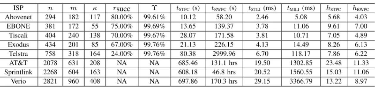
B. ISP Topologies

We also test these algorithms on real network topologies. We use the Internet Service Provider (ISP) topologies from the Rocketfuel project [25], which represent physical con-nections between backbone/gateway routers of several major ISPs around the globe. The available data do not include link performance metrics; thus, we simulate link metrics by randomly generated numbers between 0 and 1. We point out that the performance of the algorithms is independent of the values of link metrics. Since RWPC is a randomized algorithm, we repeat it for multiple Monte Carlo runs for each ISP topology and report average performance; the number of Monte Carlo runs is 100 unless otherwise stated. In this simulation, we set IMAX = 8× n since we observe that IMAX= 3×n results in zero success rate for RWPC.

Simulation results are presented in Table III, where we sort the networks according to their number of links (i.e.,n). We notice that all networks need a significantly higher ratio of monitors compared with the synthetic networks (Table II), ranging from30% (EBONE, AT&T, Sprintlink) to more than

60%(Abovenet). This is because ISP networks contain a large number of gateway routers to connect to customers or other ISPs, which appear as dangling nodes that have to be selected

TABLE II

RANDOMGRAPHS(ER:p= 0.0656, RG:dc= 0.15554, BA:ϱ= 5,IMAX= 3×n)

graph n m κ rsucc Υ tSTPC(s) tRWPC(s) tSTLI(ms) tMILI(ms) hSTPC hRWPC

ER 736.46 150 3 100.00% NA 20.2 372.61 7.39 74.58 22.16 14.35

RG 739.57 150 3.57 28.00% 91.43% 20.49 918.42 8.09 74.16 29.16 21.44

BA 732 150 3 100.00% NA 19.61 395.71 7.70 70.82 21.65 9.41

TABLE III

ISP TOPOLOGIES(IMAX= 8×nFOR THE FIRST5NETWORKS,ANDIMAX=∞FOR THE LAST3)

ISP n m κ r_succ Υ tSTPC(s) tRWPC(s) tSTLI(ms) tMILI(ms) hSTPC hRWPC

Abovenet 294 182 117 80.00% 99.61% 10.12 58.20 2.46 5.08 5.68 4.03 EBONE 381 172 55 75.00% 99.69% 13.65 139.37 3.78 11.06 9.61 7.00 Tiscali 404 240 138 70.00% 99.67% 28.07 171.58 3.81 10.71 7.05 4.89 Exodus 434 201 85 67.00% 99.76% 21.13 226.15 4.13 14.49 8.26 6.13 Telstra 758 318 164 24.00% 99.76% 80.38 2999.96 6.70 118.17 7.86 6.22 AT&T 2078 631 208 NA NA 685.46 131.1 hrs 19.50 1302.85 23.48 11.33 Sprintlink 2268 604 163 NA NA 608.18 46.8 hrs 20.52 1560.55 15.03 11.06 Verio 2821 960 408 NA NA 697.86 170.3 hrs 29.15 3366.79 13.22 8.97

as monitors; see MMP in [8] for detailed explanations. STPC again significantly outperforms RWPC with a speedup ranging from 6 fold (Abovenet, Tiscali) to 879 fold (Verio). In fact, RWPC becomes so slow for the largest three networks (AT&T, Sprintlink and Verio) that it is unable to complete a successful Monte Carlo run (r_succ = 0%) even after 40

hours. To find out the time RWPC takes to find n linearly independent paths, we remove the limitation on the number of iterations (IMAX=∞) and let it run until success. RWPC takes

up to 7 days (Verio) to complete a single Monte Carlo run7_,

which is in sharp contrast with STPC that finds n linearly independent paths in10minutes. For link identification, STLI also outperforms MILI with a speedup ranging from 2 fold (Abovenet) to 115 fold (Verio). Over all, we observe that the running-time advantages of STPC and STLI both increase with the size of the network, while the success rate and the efficiency of RWPC decay. As in the synthetic simulations, we again observe a relatively larger path length for STPC. However, the increase in path length is only moderate compared with the decrease in running time, and this is likely the cost needed to ensure linear independence of the paths.

VI. CONCLUSION

We studied the problem of network tomography from an algorithmic perspective, proposing efficient algorithms for constructing measurement paths and uniquely identifying link metrics from path measurements. The proposed algorithms uti-lize a special structure of identifiable networks in the form of independent spanning trees to strategically construct linearly independent measurement paths and compute link metrics without explicitly inverting the measurement matrix. Extensive simulations on both synthetic and real networks show that the proposed algorithms can guarantee unique identification of link metrics while being orders of magnitude faster than existing solutions for large networks.

REFERENCES

[1] F. Lo Presti, N. Duffield, J. Horowitz, and D. Towsley, “Multicast-based inference of network-internal delay distributions,” IEEE/ACM Transactions on Networking, vol. 10, no. 6, pp. 761–775, Dec. 2002. [2] M. Coates, A. O. Hero, R. Nowak, and B. Yu, “Internet tomography,”

IEEE Signal Processing Magzine, vol. 19, pp. 47–65, 2002.

[3] Y. Vardi, “Estimating source-destination traffic intensities from link data,”Journal of the American Statistical Assoc., pp. 365–377, 1996.

7_{For this reason, we only conduct one Monte Carlo run for each of these}

three networks.

[4] E. Lawrence and G. Michailidis, “Network tomography: A review and recent developments,”Frontiers in Statistics, vol. 54, 2006.

[5] O. Gurewitz and M. Sidi, “Estimating one-way delays from cyclic-path delay measurements,” inIEEE INFOCOM, 2001.

[6] Y. Chen, D. Bindel, and R. H. Katz, “An algebraic approach to practical and scalable overlay network monitoring,” inACM SIGCOMM, 2004. [7] A. Chen, J. Cao, and T. Bu, “Network Tomography: Identifiability and

Fourier domain estimation,” inIEEE INFOCOM, 2007.

[8] L. Ma, T. He, K. K. Leung, D. Towsley, and A. Swami, “Topological conditions for identifying additive link metrics via end-to-end path measurements,” Technical Report, Imperial College, London, UK, Jul. 2012. [Online]. Available: http://www.commsp.ee.ic.ac.uk/%7elm110/ pdf/MaTR1Jul12.pdf

[9] N. Duffield and F. Lo Presti, “Multicast inference of packet delay variance at interior network links,” inIEEE INFOCOM, 2000. [10] Y. Xia and D. Tse, “Inference of link delay in communication networks,”

IEEE Journal of Selected Areas in Communications, 2006.

[11] A. Adams, T. Bu, T. Friedman, J. Horowitz, D. Towsley, R. Caceres, N. Duffield, F. Presti, and V. Paxson, “The use of end-to-end multi-cast measurements for characterizing internal network behavior,”IEEE Communications Magazine, vol. 38, no. 5, pp. 152–159, May 2000. [12] R. Castro, M. Coates, G. Liang, R. Nowak, and B. Yu, “Network

tomography: recent developments,”Statistical Science, 2004.

[13] M.-F. Shih and A. Hero, “Unicast inference of network link delay distributions from edge measurements,” inIEEE ICASSP, 2001. [14] W. Xu, E. Mallada, and A. Tang, “Compressive sensing over graphs,”

inIEEE INFOCOM, 2011.

[15] A. Gopalan and S. Ramasubramanian, “On identifying additive link metrics using linearly independent cycles and paths,”IEEE/ACM Trans-actions on Networking, vol. PP, no. 99, 2011.

[16] N. Alon, Y. Emek, M. Feldman, and M. Tennenholtz, “Economical graph discovery,” inSymposium on Innovations in Computer Science, 2011. [17] G. H. Golub and C. F. Van-Loan,Matrix Computations. The Johns

Hopkins University Press, Baltimore and London, 1996.

[18] R. Diestel,Graph theory. Springer-Verlag Heidelberg, New York, 2005. [19] J. E. Hopcroft and R. E. Tarjan, “Dividing a graph into triconnected components,”SIAM Journal on Computing, vol. 2, pp. 135–158, 1973. [20] J. Cheriyan and S. N. Maheshwari, “Finding nonseparating induced cycles and independent spanning trees in 3-connected graphs,”Journal of Algorithms, vol. 9, pp. 507–537, 1988.

[21] L. Ma, T. He, K. K. Leung, D. Towsley, and A. Swami, “Efficient identification of additive link metrics: Theorem proof and evaluations,” Technical Report, Imperial College, London, UK, Nov. 2012. [Online]. Available: http://www.commsp.ee.ic.ac.uk/%7elm110/ pdf/MaTechreportNov12.pdf

[22] P. Erd¨os and A. R´enyi, “On the evolution of random graphs,” Pub-lications of the Mathematical Institute of the Hungarian Academy of Sciences, vol. 5, pp. 17–61, 1960.

[23] P. Gupta and P. Kumar, “Critical power for asymptotic connectivity in wireless networks,” Stochastic Analysis, Control, Optimization and Applications, pp. 547–566, 1999.

[24] R. Albert and A.-L. Barab´asi, “Statistical mechanics of complex net-works,”Reviews of Modern Physics, vol. 74, pp. 47–97, Jan. 2002. [25] “Rocketfuel: An ISP topology mapping engine,” University of

Washington, 2002. [Online]. Available: http://www.cs.washington.edu/ research/networking/rocketfuel/interactive/