Inference and Interpretability
in
Latent Variable Modeling
by Aritra Guha
A dissertation submitted in partial fulfillment of the requirements for the degree of
Doctor of Philosophy (Statistics)
in The University of Michigan 2020
Doctoral Committee:
Associate Professor Long Nguyen, Chair Professor Moulinath Banerjee
Assistant Professor Zhenke Wu Assistant Professor Gongjun Xu
ACKNOWLEDGEMENTS
I write this with great grief as devastating pictures of Cyclone Amphan having wreaked havoc on my beloved city crop up on my news feed. To Kolkata, the city that shall always be "home".
My PhD journey is drawing to an end. As I reflect on the past 6 years, I realise how fortunate I have been to meet and interact with so many great people each of whom have contributed significantly to my life.
First and foremost, I would like to thank my adviser, Long Nguyen, for his amazing guidance and support throughout this journey. Long has been a constant source of inspiration and positive energy, which has helped me immensely to navigate the academic challenges of PhD life. I have been constantly fascinated by his knowledgeability and depth of understanding. The innumerable interactions with him have taught me to appreciate every problem no matter how insignificant it may seem. Long is extremely caring towards his students and his door has always remained open for any query that his students may have, academic or otherwise. Time and again there have been scenarios where a brief 5-minute query has led to hours of discussions with Long, which have taught me so much about Statistics. I am also thankful to Long for introducing me to a wonderful group of peers. Long is a complete mentor. He not only ensures the appropriate academic growth of his students but also cares a lot for their mental well-being. The occasional Thanksgiving and Christmas parties have been extremely
cherishable moments and I would like to thank Long and his family for graciously hosting us so many times. Long has been the best possible adviser and an absolute role model for me, not only for his academic achievements but also for his kindness, humility and outlook towards life.
I would also like to thank Moulinath Banerjee, Gongjun Xu and Zhenke Wu for agreeing to be on my thesis defense committee, and Stilian Stoev for his invaluable advice in my first year of graduate life. I am grateful to Bodhida (Bodhisattva Sen) for his guidance over the summer of 2013 and invaluable advice over the years. Yuekai Sun, Yves Atchade and Long have also painstakingly written so many letters of recommendation for me and I cannot thank them enough for their efforts. I also take this opportunity to thank all the faculty members for their graduate courses that have shaped up my knowledge of Statistics, and all the administrative staff for their help with anything and everything I did not have a solution to. I believe that a PhD is a culmination of not just 5-6 years of work but a life time of effort from so many others who contribute in numerous ways. For that I am especially grateful to all my teachers at school (Aditya Academy and Bharatiya Vidya Bhavan) and at ISI, especially Paromita Mam, Sabita Mam and Mira Mam for shaping up my academic career.
I have had the great fortune to meet and make so many new friends in the Department. I have been extremely fortunate to have worked and interacted with Nhat, Mikhail, Rayleigh, Vincenzo, Bach, Hossein, Giuseppe, Tim, Jiahui, Jawad and so many others from whom I have learnt a lot.
Over the years at school and ISI, I have made great many friends who I have shared innumerable life experiences with: Soumya Subhra, Arkopal, Debanjan, Joydeep, Abhishek (Tewari), Sagnikda, Rupak, Paromita, Pragya, Surya, Rohit, Saketh, Avi, Soumendu, Sutanoy, Purvasha, Snehashis, Arnab (Hazra), Arkaprava, Sayan, Rudrendu,
Abir, Deepanjan, Suprajo and so many more. I am forever indebted to each and every one of them for their support throughout my life. I am honored to have found an amazing family away from home in Ann Arbor: Anwesha, Diptavo, Rounakda, Shrijitadi, Avijitda, Debarghya, Subha, Rupam, Debraj, Soumik, Moulida and Bharamardi, thank you for the countless adda sessions and late night hangouts and coffee chats. I am also grateful to all the members of Ann Arbor and Troy cricket fraternities for the camraderie and all the cricket outings. They definitely made the summers all that more exciting.
Finally, this thesis is dedicated to my family. I would like to express my deep gratitude to my parents, Aruna and Abhijit Guha for their selfless love, unconditional sacrifice, support and belief in me since the day I was born. I would like to thank all my family members for their love, and especially my grandmother Binapani Dattagupta, and my uncles Arup and Barun Dattagupta for their guidance in life. I consider myself extremely lucky to have met Swagata. I am grateful to her for all the love and support over the past few years and for all the discussions on realities and perspectives. Her presence made the dark times a lot brighter. Special thanks also go to my brother, Arkajit for bearing with all my tantrums and leg-pullings over the past 23 years of life. Last but not the least, I am especially thankful to Jethu, Nandadulal Datta for instilling in me the love for Mathematics and for teaching me about circles. I would never have made it this far if not for his guidance during my school years. To end, I would like to iterate one of Jethu’s numerous one-liners, "God is a circle whose center is everywhere, circumference nowhere".
TABLE OF CONTENTS
DEDICATION ii
ACKNOWLEDGEMENTS iii
LIST OF FIGURES x
LIST OF TABLES xiv
ABSTRACT xv
CHAPTER
I. Introduction . . . 1
1.1 Model complexity, estimation and interpretability in Bayesian mixture modeling . . . 3
1.2 Scalable and efficient geometric algorithms for probabilistic models 7 1.3 Evaluation of primitive scenarios for autonomous vehicles . . . 11
1.4 Thesis Organization . . . 12
II. Posterior Contraction of Parameters and Interpretability in Bayesian Mixture Modeling . . . 14
2.1 Introduction . . . 15
2.1.1 Well-specified regimes . . . 18
2.1.2 Misspecified regimes . . . 22
2.1.3 Further remarks . . . 25
2.2 Preliminaries . . . 27
2.3 Posterior contraction under well-specified regimes . . . 30
2.3.2 Optimal posterior contraction via a parametric Bayesian
mixture . . . 33
2.3.3 A posteriori processing for BNP mixtures . . . 37
2.4 Posterior contraction under model misspecification . . . 42
2.4.1 Gaussian location mixtures . . . 46
2.4.2 Laplace location mixtures . . . 50
2.4.3 When G∗ has finite support . . . 56
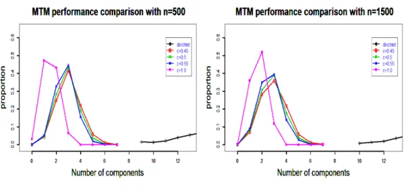
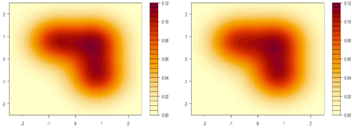
2.5 Simulation studies . . . 59
2.6 Appendix A: Proofs of key results . . . 64
2.6.1 Proof of Theorem 2.3.1 . . . 64
2.6.2 Posterior consistency of Merge-Truncate-Merge algorithm 71 2.6.3 Proof of Lemma 2.4.3 . . . 83
2.6.4 Proof of Proposition 2.4.1 . . . 85
2.6.5 Proof of Proposition 2.4.2 . . . 88
2.7 Appendix B: Weighted Hellinger and Wasserstein distance . . . 92
2.7.1 Proof of Lemma 2.4.2 . . . 93
2.7.2 Proof of Proposition 2.4.3 . . . 93
2.8 Appendix C: Posterior contraction under misspecification . . . 96
2.9 Appendix D: Proofs of remaining results . . . 100
2.9.1 Proof of Theorem 2.4.1 . . . 100
2.9.2 Proof of Lemma 2.8.2 . . . 102
2.9.3 Proof of Theorem 2.8.2 . . . 103
2.9.4 Proof of Lemma 2.8.1 . . . 107
2.9.5 Proof of Theorem 2.4.3 . . . 109
III. Bayesian Contraction for Dirichlet Process Mixtures of Smooth Densities . . . 113
3.1 Introduction . . . 114
3.2 Preliminary . . . 120
3.3 Sieve methods via growing parameter space . . . 122
3.3.1 Lower bound of Hellinger distance based on Wasserstein metric . . . 123
3.3.2 Growing parameter space . . . 127
3.4 Contraction of excess mass for Gaussian mixtures . . . 133
3.5 Simulation Studies . . . 147
3.6 Appendix A: Proofs . . . 151
3.6.1 Proof of Theorem 3.3.2 . . . 151
3.6.2 Proof of Theorem 3.3.4 . . . 155
3.7 Appendix B: Auxiliary results . . . 164
3.7.1 Proof of Theorem 3.3.1 . . . 164
3.7.2 Proof of Theorem 3.3.3 . . . 173
3.7.3 Prior mass on Wasserstein ball . . . 177
3.7.4 Metric Entropy with Hellinger distance . . . 177
3.7.5 Computation of M corresponding to KL ball . . . 180
3.7.6 Equivalence of Hellinger and Wasserstein metrics for Laplace location mixtures . . . 184
IV. Dirichlet Simplex Nest and Geometric Inference. . . 187
4.1 Introduction . . . 187
4.2 Dirichlet Simplex Nest . . . 191
4.3 Inference of the Dirichlet Simplex Nest . . . 193
4.3.1 Simplicial Geometry . . . 193
4.3.2 The Voronoi Latent Admixture (VLAD) Algorithm . 196 4.3.3 Estimating the Dirichlet Concentration Parameter . . 199
4.4 Consistency and Estimation Error Bounds . . . 200
4.5 Experiments . . . 203
4.5.1 Comparative Simulation Studies . . . 204
4.5.2 Real Data Analysis . . . 207
4.6 Summary and Discussion . . . 208
4.7 Appendix . . . 210
4.7.1 Proofs of Theorems . . . 210
4.7.2 Experimental Details . . . 222
4.7.3 On asymmetric Dirichlet prior . . . 226
V. Robust Representation Learning of Temporal Dynamic Inter-actions . . . 228
5.1 Introduction . . . 229
5.2 A distance metric on temporal interactions . . . 234
5.2.1 Rotation and translation-invariant metrics on curves . 235 5.3 Quantifying distributions of primitives . . . 239
5.3.1 Wasserstein barycenter and k-means clustering . . . . 241
5.3.2 Approximations for non-Euclidean k-means clustering 243 5.4 Experimental Results . . . 246
5.4.1 Vehicle-to-vehicle (V2V) interaction data processing . 247 5.4.2 Cluster analysis of V2V interactions . . . 250
5.5 Conclusion . . . 259
5.6 Appendix . . . 260
5.6.1 Proofs . . . 260
5.6.2 Obtaining primitives via splines . . . 263
5.6.3 Algorithm for centering and reorienting primitives . . 264
VI. Conclusions and Future Work . . . 267
6.1 A velocity flow model to analyse traffic movements . . . 268
6.2 Misspecification in the number of mixture model components . 269 6.3 Statistical efficiency of Variational Inference for hierarchical Bayesian models . . . 271
6.4 Geometric inference for hierarchical models . . . 271
LIST OF FIGURES
Figure
1.1 K topics, M documents,Nm exchangeable words in each document w 8
1.2 Toy example of LDA . . . 9
2.1 Initial distribution G. . . 59
2.2 After first stage-"merge". . . 59
2.3 After second stage-"truncation". . . 59
2.4 After second stage-"merge". . . 59
2.5 Case A. . . 61
2.6 Case B. . . 61
2.7 Case C. . . 63
2.8 Case D. . . 63
3.1 truth is mixture of light-tail kernel, fit with mixture of light-tail. . . . 149
3.2 truth is mixture of heavy-tail kernel, fit with mixture of light-tail . . . 149
3.3 Fitting with Gaussian . . . 149
3.4 truth is mixture of light-tail kernel, fit with mixture of heavy-tail . . . 149
3.5 truth is mixture of heavy-tail kernel, fit with mixture of heavy-tail . . 149
3.6 Fitting with Student’s t . . . 149
4.1 GDM; time ≈ 1s . . . 190
4.2 Xray; time < 1s . . . 190
4.3 HMC; time ≈ 10m . . . 190
4.4 VLAD; time < 1s . . . 190
4.5 Toy simplex learning: n= 5000, D = 3, K = 3, α= 2.5, σ = 0.1. . . 190
4.6 Gaussian data . . . 205
4.7 Poisson data . . . 205
4.8 Categorical data . . . 205
4.9 Minimum matching distance for increasing n . . . 205
4.10 Gaussian data . . . 206
4.11 Poisson data . . . 206
4.13 Minimum matching distance for varying DSN geometry. . . 206
4.14 Gaussian data . . . 206
4.15 Poisson data . . . 206
4.16 Categorical data . . . 206
4.17 Minimum matching distance for increasing α. . . 206
4.18 Empirical study of α identifiability. . . 221
4.19 Frobenius norm for Gaussian data . . . 222
4.20 Negative log-likelihood for Poison data . . . 222
4.21 Perplexity for LDA data . . . 222
4.22 Held out data performance for increasing sample size n . . . 222
4.23 Frobenius norm for Gaussian data . . . 223
4.24 Negative log-likelihood for Poison data . . . 223
4.25 Perplexity for LDA data . . . 223
4.26 Held out data performance for varying DSN geometry . . . 223
4.27 Frobenius norm for Gaussian data . . . 223
4.28 Negative log-likelihood for Poison data . . . 223
4.29 Perplexity for LDA data . . . 223
4.30 Held out data performance for increasing α . . . 223
4.31 GDM . . . 227
4.32 Xray . . . 227
4.33 HMC . . . 227
4.34 VLAD . . . 227
4.35 Asymmetric Dirichlet toy simplex learning: n = 5000, D = 3, K = 3, α= (0.5,1.5,2.5) . . . 227
5.1 Multidim. Scaling (cf. Section 5.3.2.1) . . . 248
5.2 First geometric approx. (cf. Section 5.3.2.2) . . . 248
5.3 Second geometric approx. (cf. Section 5.3.2.2) . . . 248
5.4 Polynomial coefficients (cf. Section 5.4.2) . . . 248
5.5 DTW cost matrix (cf. Wang and Zhao (2017)) . . . 248
5.6 Silhouette plots for 5 clusters obtained under various approaches: . . 248
5.7 Cluster 1 . . . 251 5.8 Cluster 2 . . . 251 5.9 Cluster 3 . . . 251 5.10 Cluster 4 . . . 251 5.11 Cluster 5 . . . 251 5.12 All clusters . . . 251
5.13 Plot of the three most typical interactions organized from the cluster with the most interaction to the cluster with the fewest for clustering using Multidimensional scaling (cf. Section 5.3.2). The interactions are centered and oriented using Algortihm 5.4 to (t,2t−1,−t,1−2t)for t = 0,0.01, . . . ,1. The solid shapes and shapes with a black interior indicate the starting location of each interaction. The dot with the black interior indicates the second trajectory. Midpoints are indicated by dots filled in with a grey interior. Different shapes indicate different V2V interactions. Note that the individual cluster interactions plots
are placed on their own scales. . . 251
5.14 In-cluster distances from mean interactions . . . 252
5.15 In-cluster distances from typical interactions . . . 252
5.16 All distances from mean interactions . . . 252
5.17 All distances from typical interactions . . . 252
5.18 In-cluster distances from the mean interactions . . . 252
5.19 In-cluster distances from the typical interactions . . . 252
5.20 All distances from mean interactions . . . 252
5.21 All distances from the typical interactions . . . 252
5.22 In-cluster from mean interactions . . . 252
5.23 In-cluster distances from typical interactions . . . 252
5.24 All distances from mean interactions . . . 252
5.25 All distances from typical interactions . . . 252
5.26 Line plots showing the distribution (frequency) of interaction distance to either the cluster mean or the typical interaction. Clusters are obtained by the first geometric method in row 1, the second geometric method in row 2, and the cubic spline coefficients based method in row 3 (cf. Section 5.4.2). The clusters are numbered according to the number of interactions so that Cluster 1 has the most and Cluster 5 has the fewest. Note that the range for the y-axis are much larger on the left plots compared to the right plots. . . 252
5.27 All k and β between 2 and 20 . . . 257
5.28 All β between 10and 20 and k between 10and 20 . . . 257
5.29 All β between 2 and 20 and k between 10 and 20 . . . 257
5.30 All β between 2and 20 and k between 10 and 20 . . . 257
5.31 The left two plots show heatmaps of the statistic introduced in Eq. (5.15) for encounters segmented by the two-step spline approach (cf. Appendix 5.6.2) and then clustered via MDS (cf. Section 5.3.2). The right two show changes in this statistic. . . 257
5.32 MDS clustering (cf. Section 5.3.2) applied to two-step spline segmented encounters (cf. Appendix 5.6.2). . . 257
5.33 DTW matrix clustering applied to encounters segmented by BNP (cf.
Wang and Zhao (2017)). . . 257
5.34 Two step spline segmented encounters clustered using primitives ex-tracted from BNP segmented encounters clustered using DTW matrices (cf. 5.4.3). . . 257
5.35 Heatmaps of the statistic given by Eq. (5.15) for non-reflective Pro-crustes distance for k ≥10across different methods. . . 257
5.36 Multidim. scaling approach (cf. Section 5.3.2.1) . . . 265
5.37 First geometric approx. (cf. Section 5.3.2.2) . . . 265
5.38 Second geometric approx. (cf. Section 5.3.2.2) . . . 265
5.39 Polynomial coefficients (cf. Section 5.4.2) . . . 265
5.40 DTW cost matrix (cf. Wang and Zhao (2017)) . . . 265
5.41 Plot of the three most typical interactions organized from the cluster with the most interaction to the cluster with the fewest for various methods. See Figure 5.13 for the legend and for how the interactions are oriented. . . 265
LIST OF TABLES
Table
4.1 Baselines and required conditions . . . 205 4.2 NYT topic modeling (categorical data) . . . 207 4.3 Stock data factor analysis (continuous data) . . . 207 5.1 A table of the quantities from Eq. (5.8), Eq. (5.11), and Eq. (5.13)) for
each method’s cluster with the most interaction (Cluster 1) and cluster with the fewest (Cluster 5). Variance of these distances are included in parentheses. Note that the Procrustes distances were normalized so that the maximum distance between any interaction is 1. . . 248
ABSTRACT
In this age of technology, more and more data is generated as an outcome of complex processes through heterogeneous mechanisms. Statistical models therefore need to invoke the complexities for appropriate inference. One such situation is when data is generated from heterogeneous sub-populations. Hierarchical models form the state-of-the-art methods for such scenarios. However, Markov Chain Monte Carlo methods, which form the traditional inference method can be quite cumbersome to implement for such large scale models, resulting in high time complexities. Sometimes, they may also suffer from inconsistency issues. On the other hand, mean-field variational inference methods even though fast, can suffer from inaccuracy in estimation. This dissertation focuses on understanding such complex models and drawing inference from each of those sub-populations and develops alternative techniques for inference, with statistical guarantees.
Our specific contributions are as follows. We provide an in-depth analysis of two specific types of latent variable models, namely, mixture and admixture models and also develop an unsupervised learning scheme with applications to autonomous vehicles.
In the mixture model context, firstly, we develop an understanding of the posterior contraction behavior of parameter estimation in the case of infinite mixture models, corresponding to two choices of priors, one parametric and the other nonparametric. Next, we provide an in-depth analysis of Bayesian mixtures under various misspecification settings and provide an asymptotic characterization pertaining to such scenarios. Our
study reveals a deep perception of the role, the kernel plays on the statistical decisions of a practitioner. Next, in the context of admixture models, we develop a geometric estimation mechanism to the well-known Latent Dirichlet Allocation model. Finally, we provide a model-free inference scheme to robustly estimate and evaluate parameters of various sub-populations, in the applied setting when the heterogeneous sub-populations for data generation are derived from car driving scenarios, via the use of unsupervised learning.
CHAPTER I
Introduction
With the advent of technology, a large amount of today’s data is generated by means of complex mechanisms. Data may be available in various forms - for example, unlabelled data as in images, tweets, articles or time series data as in daily weather reports, traffic scenarios including but not limited to inter-vehicular interactions. Moreover, data available is often high-dimensional in nature as vast amount of information is generated at low costs. For example, large-scale biological datasets obtained through next-generation sequencing, proteomics or brain-imaging are often high-dimensional. Other kinds of data may be more personal in nature, such as mobile app based monitoring of driving, health or other individual-specific activities. Any suitable Statistical method therefore needs to be considerate of the appropriate complexities of the data involved, for efficient inference. The accommodations of appropriate Statistical models are two-fold. Firstly, the model should be mindful of the heterogeneity of the processes and be suitable for inferring from each of the subpopulations in the data-generating scheme. Secondly, the inference scheme should also be scalable for large dimensional data. Unsupervised learning schemes such as probabilistic Principal component analysis (cf. Tipping and Bishop (1999); Roweis and Ghahramani (1999)), Factor analysis (cf.Anderson and Rubin (1956)), Independent
component analysis (cf. Hyvärinen et al.(2004)) are well-known scalable techniques for large datasets. Ghahramani (2004) provides a succint account of unsupervised learning techniques. However, they often fail to capture the heterogeneity of the data because of their model-free constitution. On the other hand, Bayesian hierarchical models such as Mixture models (cf. McLachlan and Basford (1988)), Admixtures (cf. Pritchard et al.
(2000)), Hierarchical Dirichlet processes (HDP) (cf. Teh et al. (2006)), Hidden Markov models (cf. Baum and Petrie (1966); Baum et al. (1970)) form the state-of the-art methods for modelling of heterogeneous subpopulations. However, they may suffer from inconsistency issues (cf. Miller and Harrison (2014)). Markov Chain Monte Carlo algorithms (cf. Griffiths and Steyvers (2004);Escobar and West (1995);MacEachern and Mueller (1998); Neal (2000); Teh et al. (2006); Fox et al.(2009)) form the state-of-the-art methods for inference with hierarchical models. However, a large number of latent variables in combination with complex modeling structures often makes it difficult for MCMC algorithms to be scalable. A useful alternative is provided by Variational Inference algorithms (cf. Jordan et al. (1999); Blei et al. (2003); Blei and Jordan
(2006); Hoffman et al. (2013); Mandt et al. (2017)). Several recent papers (cf. Wang and Blei (2018, 2019)) explore the asymptotic consistency for Variational Inference algorithms. However, finite sample outcomes for VI algorithms do not produce the accurate Posterior distribution. Moreover, asymptotic consistency cannot be guaranteed for graphical models with complex structures. As a result, the need for scalable and statistically efficient algorithms is ever-present. This thesis focuses on understanding inference-related questions for such complex models and develops appropriate techniques for scalable inference with statistical guarantees. For this work, our focus is only on mixture and admixture models.
Relevant background material is included in each section to make the sections self-contained.
1.1
Model complexity, estimation and interpretability in Bayesian
mixture modeling
Mixture models form the basic building blocks in latent variable modeling and provide an interpretable way for a statistician to analyze data from heterogeneous population sources (cf.McLachlan and Basford (1988);Lindsay (1995);Mengersen et al.
(2011)). With practical applicability in model-based clustering techniques and modeling complex distributions(cf. McLachlan and McGriffin (1994)), mixture models provide a wide range of scopes for statistical modeling. Mixture models view data as samples from an assembly of latent sub-populations, each assuming its own distribution with corresponding parameters.
More concretely, we work with the following specific formulation of mixture models. Consider discrete mixing measures G=Pk
i=1piδθi. Here, p= (p1, . . . , pk)is a vector of
mixing weights, while atoms {θi}k
i=1 are elements in a given compact space Θ. Mixing measure G is combined with a kernel function f(·|θ)with respect to Lebesgue measure µ to yield a mixture density:
pG(·) = Z f(·|θ)dG(θ) = k X i=1 pif(·|θi).
When k <∞, we call this a finite mixture model with k components. For an infinite mixture model, k is allowed to take the value ∞.. The atoms θi’s are representatives of the underlying subpopulations.
The choice of the kernel f, and the prior on the unknown distribution G, affect the outcome of inference drastically for a practitioner of Bayesian mixture models. For a Bayesian, the choice of priors for mixture models is essentially restricted to two primary options:
(i) a nonparametric prior via use of Dirichlet process distribution on the mixing measures.
(ii) a parametric counterpart of Dirichlet process mixtures via use of suitable priors (eg. Poisson) on number of components.
Estimation of the true but unknown number of mixture components is an important inference question relative to mixture models. The choice of the prior drastically influences the efficiency of estimation corresponding to the parameters representing these components. A common misconception that may have initially contributed to the enthusiasm for Bayesian nonparametric modeling is that the use of such nonparametric models eliminates altogether the need for determining the number of mixture components, because the learning of such a quantity is "automatic" from the posterior samples of the mixing measure. However, Miller and Harrison (2014) explicitly demonstrated that the common practice of drawing inference about the number of mixture components via the DP mixture by counting the number of support points in the sample of the Dirichlet posterior leads to an asymptotically inconsistent estimate.
With this in context, we propose Merge-Truncate-Merge in Chapter II of this thesis. It is a post-processing algorithm that resolves the inconsistency issue by allowing to consistently estimate the true number of components with Dirichlet process mixtures. Moreover, the algorithm outputs posterior samples that retain the original parameter contraction rates pertaining to samples from the Dirichlet process posterior. Additionally,
we also show that the parametric choice of prior given in (ii) yields optimal rates of convergence of the mixing measure (up to a logarithmic term), in addition to correctly recovering the number of mixture components, under considerably weak conditions.
Following George Box’s famous quote, "all models are wrong, but some are useful", a natural question that may arise in the context of inference related to mixtures is: what happens to a mixture model based statistical procedure when the model is actually misspecified?
Misspecification may be of various different categories. Misspecifications of the kernel may skew the performance of the methods in question and lead to an incorrect conclusion because of non-robustness properties of the model. With regard to interpretability of parameter estimation under the misspecified model regime, our results reveal several new insights. Given the model is misspecified, the statistician might choose to indulge in heavy-tailed kernels which allow for fast contraction of parameter estimates, thereby implying that a given data set probably has relatively faster influence on the movement of mass from the prior to the posterior distribution. In that regard, Laplace location mixtures may be preferred to Gaussian location mixtures, provided that the bias due to misspecification is not too large. On the other hand, when this is not the case, it is advisable to have a more "conservative" approach by adopting Gaussian kernels instead, despite the latter’s lagging posterior contraction behavior. Overall, the ultimate model choice under misspecification will reside on resolving the tension between the aforementioned bias and contracting variance.
Other kinds of misspecifications may arise out of a biased choice for the support of the prior. Theoretical results often rely on critical assumptions which may create such scenarios in practice. For example, a vast array of works that deal with asymptotically optimal estimation procedures for the population density (cf. Ghosal et al. (1999);
Ghosal and van der Vaart (2007);Shen et al. (2013)) rely on the critical assumption that the space of parameters is bounded. It is also a common assumption for works that deal with the theoretical understanding of the parameter estimation regime (cf. Nguyen
(2013);Gao and van der Vaart (2016);Scricciolo (2017)). However, such an assumption may be unfavorable in situations where this bounded support in incorrectly specified. While a small support allows for misspecification of the parameter space thereby leading to a bias in estimation, a large or unbounded support leads to a slow contraction rate thereby resulting in higher variability in estimation. In practice, it is common to allow the base prior for the parameters to have an unbounded support to overcome the additional step of estimating the support of the prior. As a result there is a glaring mismatch between the practical application and theoretical understanding for parameter estimation problems with Bayesian nonparametric priors. In Chapter III of this thesis, we provide a solution to this problem via the use of sieve estimates.
Sieve methods have been implemented in the density estimation context by many authors such as Ghosal and van der Vaart (2001); Shen and Wong (1994); Wong and Shen (1995); Van de Geer (1993); Birge and Massart (1998). However, to the best of our knowledge, there has been no such treatment in the context of parameter estimation. As part of the sieve estimation procedure we allow the support of the prior to change gradually with the sample-size. This enables us to overcome the bias in parameter estimation while appropriately increasing the variance at a suitably chosen rate, thereby providing a solution to the eternal bias-variance trade-off problem in this context. Our theory reveals that this rate of change of support is much faster when the chosen kernel is light-tailed as compared to heavy-tailed ordinary smooth kernels. This might be counterintuitive to the results in Chapter II since it implies that for supersmooth kernels a possible large change in bias of estimation results in only a relatively negligible change
in variance. To address this puzzling issue, we develop a novel metric that generalizes the well-known Wasserstein metric, which is the popular choice of metric for parameter estimation. The use of this novel metric, which we call the "Orlicz-Wasserstein distance", leads us to a deeper understanding of the behavior of the posterior atoms. We show that for light-tailed kernels, the posterior atoms highly populate the neighbourhood of the true atoms with little contribution from other regions of the parameter space. As a result, the contribution to the variance mostly arises from the neighbourhoods of true atoms. Therefore, beyond a certain point, change in variance is affected marginally by change in bias.
1.2
Scalable and efficient geometric algorithms for probabilistic
models
Hierarchical and latent variable models broaden the scope of inference. However, a key challenge with the use of hierarchical models is fast and efficient computation of hyperparameters, both in the parametric and nonparametric context. The meaningful inferential and methodological questions involved in hierarchical modeling are:
(I) Can we have a generic modeling scheme which encompasses a large number of data generating procedures?
(II) Can we efficiently estimate the parameters of the models under the knowledge or lack thereof of the number of latent subpopulations?
Scalable estimation for parametric models: For many complex probabilistic models, especially those with latent variables, the probability distribution of interest can be represented as an element of a convex polytope in a suitable ambient space, for
which model fitting may be cast as the problem of finding the extreme points of the polytope. For instance, a mixture density can be identified as a point in a convex set of distributions whose extreme points are the mixture components. The well-acclaimed Latent Dirichlet Allocation (LDA) (cf. Blei et al. (2003)) model, which is used for analysis of text data, is another example of such a model. In the following, we provide a brief overview of the LDA model.
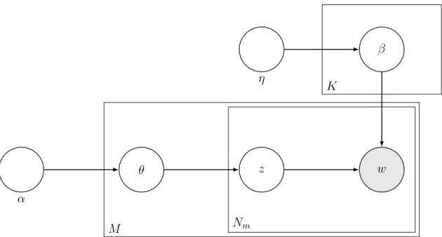
α θ z w β η M Nm K
Figure 1.1: K topics, M documents,Nm exchangeable words in each document w
Latent Dirichlet Allocation Figure 1.1 provides a graphical model description of the LDA model. The generative process of the model can be described as follows.
Consider a corpus of M documents with V denoting the number of words in the vocabulary. Suppose there are K topics. Let α ∈ RK
+, η ∈ RV+ be the respective hyperparameters corresponding to the topic distributions in a document and the word
Word 1 Word 2 Word 3 Word 4
p
mw¯
mβ
3β
2β
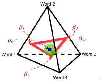
1 ;Figure 1.2: Toy example of LDA
distributions in a topic respectively. The topics are generated as follows:
βk|η∼DirV(η), fork = 1, . . . , K.
For each of the M documents, generate a topic proportionality vector as:
θm|α∼DirV(α), for m= 1, . . . , M. (1.1)
For each of the Nm words in documentm, generate a topic labelz, and a sample word d from the corresponding topic as:
zn|θm ∼ Cat(θm); dn|zn ∼ Cat(βzn) forn = 1, . . . , Nm. (1.2)
Admixture model (cf. Pritchard et al. (2000)), which is popular in genetics is equivalent to the LDA model. The LDA model embeds the topic distributions in the probability simplex and therefore is convenient for word-document frequency distributions. This
simplicial structure of the model is amenable to efficient inference and therefore prove useful for other datatypes as well. In Chapter IV, we propose Dirichlet Simplex Nest (DSN), a class of probabilistic models that generalizes the Latent Dirichlet Allocation.
By viewing data as noisy observations from the low-dimensional affine hull that contains a simplex, our model shares an assumption that can be found in classical factor analysis, non-negative matrix factorization (NMF) models (cf. Lee and Seung (2001)), as well as in topic models (cf. Arora et al.(2012b)). The class of models provides a probabilistic justification for these methods, which often impose an additional geometric condition on the model known as separability that identifies the model parameters in a way that permits efficient estimation (cf. Arora et al. (2012a)). Moreover the DSN modeling provides an arguably more effective approach to archetypal analysis and non-negative matrix factorization for non-separable data as well.
The key challenge for inference using the DSN model lies in scalable and efficient parameter estimation. While Hamiltonian Monte Carlo lacks scalability guarantees for such complexly structured models, NMF algorthms perform poorly when theseparability
condition cannot be guaranteed. Variational Inference (cf. Blei et al. (2003)) forms the go-to scalable algorithm for inference with the LDA model.However, the questions of statistical efficiency with Variational Inference algorithms remain mostly unexplored. Starting with an original geometric technique of Yurochkin and Nguyen (2016), we provide in Chapter IV Voronoi Latent Admixture (VLAD) algorithm, a novel inference algorithm that accounts for the convex geometry and low dimensionality of the latent simplex structure endowed with a Dirichlet distribution. This allows for more effective learning of asymmetric simplicial structures and the Dirichlet’s concentration parameter for the general DSN model, and hence, expands its applicability to a broad range of data distributions. More specifically, VLAD can be used for scalable and efficient estimation
corresponding to the LDA model setup with greater accuracy than the state-of-the-art Variational Inference algorithms. We also establish statistical consistency and estimation error bounds for the proposed algorithm.
1.3
Evaluation of primitive scenarios for autonomous vehicles
While model-based inference schemes provide increased interpretability, they can often be computationally expensive, especially for huge datasets. Moreover, structural specificity of models may often hinder the general applicability of model-based schemes. On the other hand, model-free mechanisms find a wider variety of applications.
In autonomous vehicle research, there has been a lot of work dedicated to understand-ing traffic scenarios. Analysis and recognition of drivunderstand-ing styles are profoundly important to intelligent transportation and vehicle calibration. Unfortunately, it can be hard to manually select a representative subset of scenarios or potentially computationally expensive to annotate them because of limited prior knowledge. Several recent papers employ unsupervised and empirical approaches to extract primitive driving patterns from time series driving data without prior knowledge of the number of these patterns (cf. Wang and Zhao (2017);Taniguchi et al.(2015);Bender et al. (2015)). However, this wide variety of unsupervised approaches leads to the obvious question of which method to choose.
With regards to that we develop a geometric invariant metric to compare different driving scenarios in Chapter V of this thesis. This novel metric is generally applicable and therefore can be easily extended to evaluate cluster efficiencies and stabilities of the existing clustering methods.
traffic driving encounters as objects. We propose a general framework to understand distributional patterns in driving styles and provide an approximate solution for clustering the distributional behavior via unsupervised learning techniques. Additionally, the method provided is robust and model-free and therefore has a wider scope of application beyond the specific dataset considered.
1.4
Thesis Organization
The remainder of this thesis proceeds as follows:
Chapter II: Posterior contraction of parameters and interpretability in Bayesian mixture modeling This chapter addresses several key issues concern-ing Bayesian nonparametric mixture models such as the inestimability of the number of components with Dirichlet Process priors, and develops an understanding of the behavior of the mixture models in the misspecified regime.
Chapter III: Bayesian contraction for Dirichlet process mixtures of smooth densities This chapter proposes a solution for the problem of misspecification of the underlying parameter space via the use of sieve estimates, and develops a deeper understanding of the behavior of mixtures of smooth kernels.
Chapter IV: Dirichlet Simplex Nest and Geometric Inference This chapter introduces a general modeling framework for inference via a generalization of the well-known Latent Dirichlet Allocation Model and provides a solution for computationally and statistically efficient inference.
Chapter V: Robust Representation Learning of Temporal Dynamic Interac-tions This chapter proposes a framework to analyse the behavior of unsupervised clustering approaches with application to traffic encounters, and also provides a novel clustering approach for the same.
Chapter VI: Conclusions and Future Work This chapter summarizes the novel contributions of this thesis and discusses idea for future research.
Each chapter is self-contained with all the necessary background materials and can be read independently of other chapters.
CHAPTER II
Posterior Contraction of Parameters and
Interpretability in Bayesian Mixture Modeling
We study posterior contraction behaviors for parameters of interest in the context of Bayesian mixture modeling, where the number of mixing components is unknown while the model itself may or may not be correctly specified. Two representative types of prior specification will be considered: one requires explicitly a prior distribution on the number of mixture components, while the other places a nonparametric prior on the space of mixing distributions. The former is shown to yield an optimal rate of posterior contraction on the model parameters under minimal conditions, while the latter can be utilized to consistently recover the unknown number of mixture components, with the help of a fast probabilistic post-processing procedure. We then turn the study of these Bayesian procedures to the realistic settings of model misspecification. It will be shown that the modeling choice of kernel density functions plays perhaps the most impactful roles in determining the posterior contraction rates in the misspecified situations. Drawing on concrete posterior contraction rates established in this paper we wish to highlight some aspects about the interesting tradeoffs between model expressiveness and interpretability
that a statistical modeler must negotiate in the rich world of mixture modeling. 1.
2.1
Introduction
Mixture models are one of the most useful tools in a statistician’s toolbox for analyzing heterogeneous data populations. They can be a powerful black-box modeling device to approximate the most complex forms of density functions. Perhaps more importantly, they help the statistician express the data population’s heterogeneous patterns and interpret them in a useful way (McLachlan and Basford (1988); Lindsay
(1995); Mengersen et al.(2011)). The following are common, generic and meaningful questions a practitioner of mixture modeling may ask:
(I) how many mixture components are needed to express the underlying latent sub-populations.
(II) how efficiently can one estimate the parameters representing these components. (III) what happens to a mixture model based statistical procedure when the model is
actually misspecified?
How to determine the number of mixture components is a question that has long fascinated mixture modelers. Many proposed solutions approached this as a model selection problem. The number of model parameters, hence the number of mixture components, may be selected by optimizing with respect to some regularized loss function; see, e.g., Lindsay (1995); Kass and Raftery (1995); Dacunha-Castelle and Gassiat (1997) and the references therein. A Bayesian approach to regularization is to place explicitly a prior distribution on the number of mixture components, e.g., Nobile
(1994);Richardson and Green (1997);Nobile and Fearnside (2007); Miller and Harrison
(2018). A convenient aspect of separating out the modeling and inference questions considered in (I) and (II) is that once the number of parameters is determined, the model parameters concerned by question (II) can be estimated and assessed via any standard parametric estimation methods.
In a number of modern applications of mixture modeling to heterogeneous data, such as in topic modeling, the number of mixture components (the topics) may be very large and not necessarily a meaningful quantity (Blei et al. (2003); Tang et al. (2014)). In such situations, it may be appealing for the modeler to consider a nonparametric approach, where both (I) and (II) are considered concurrently. The object of inference is now the mixing measure which encapsulates all unknowns about the mixture density function. There were numerous works exemplifying this approach, for eg., Leroux (1992);
Figueiredo and Jain (1993); Ishwaran et al. (2001). In particular, the field of Bayesian nonparametrics (BNP) has offered a wealth of prior distributions on the mixing measure based on which one can arrive at the posterior distribution of any quantity of interest related to the mixing measure (Hjort et al.(2010)).
A common choice of such priors is the Dirichlet process (Ferguson (1973);Blackwell and MacQueen (1973); Sethuraman (1994)), resulting in the famous Dirichlet process mixture models (Antoniak (1974);Lo(1984);Escobar and West (1995)). Dirichlet process (DP) and its variants have also been adopted as a building block for more sophisticated hierarchical modeling, thanks to the ease with which computational procedures for posterior inference via Markov Chain Monte Carlo can be implemented (Teh et al.
(2006); Rodriguez et al.(2008)). Moreover, there is a well-established asymptotic theory on how such Bayesian nonparametric mixture models result in asymptotically optimal estimation procedures for the population density. See, for instance, Ghosal et al.(1999);
Ghosal and van der Vaart (2007); Shen et al. (2013) for theoretical results specifically on DP mixtures, and Ghosal et al. (2000); Shen and Wasserman (2001); Walker et al.
(2007) for general BNP models. The rich development in both algorithms and theory in the past decades has contributed to the widespread adoption of these models in a vast array of application domains.
For some time there was a misconception among quite a few practitioners in various application domains, a misconception that may have initially contributed to their enthusiasm for Bayesian nonparametric modeling, that the use of such nonparametric models eliminates altogether the need for determining the number of mixture components, because the learning of such a quantity is "automatic" from the posterior samples of the mixing measure. The implicit presumption here is that a consistent estimate of the mixing measure may be equated with a consistent estimate of the number of mixture components. This is not correct, as has been noted, for instance, by Leroux (1992) in the context of mixing measure estimation. More recently, Miller and Harrison (2014) explicitly demonstrated that the common practice of drawing inference about the number of mixture components via the DP mixture, specifically by reading off the number of support points in the Dirichlet’s posterior sample, leads to an asymptotically inconsistent estimate.
Despite this inconsistency result, it will be shown in this chapter that it is still possible to obtain a consistent estimate of the number of mixture components using samples from a Dirichlet process mixture, or any Bayesian nonparametric mixture, by applying a simple and fast post-processing procedure on samples drawn from the DP mixture’s posterior. On the other hand, the parametric approach of placing an explicit prior on the number of components yields both a consistent estimate of the number of mixture components, and more notably, an optimal posterior contraction rate for
component parameters, under a minimal set of conditions. It is worth emphasizing that all these results are possible only under the assumption that the model is well-specified, i.e., the true but unknown population density lies in the support of the induced prior distribution on the mixture densities.
As George Box has said, "all models are wrong", but more relevant to us, all mixture models are misspecified in some way. The statistician has a number of modeling decisions to make when it comes to mixture models, including the selection of the class of kernel densities, and the support of the space of mixing measures. The significance of question (III) comes to the fore, because if the posterior contraction behavior of model parameters is very slow due to specific modeling choices, one has to be cautious about the interpretability of the parameters of interest. A very slow posterior contraction rate in theory implies that a given data set probably has relatively very slow influence on the movement of mass from the prior to the posterior distribution.
In this chapter we study Bayesian estimation of model parameters with both well-specified and miswell-specified mixture models. There are two sets of results. The first results resolve several outstanding gaps that remain in the existing theory and current practice of Bayesian parameter estimation, given that the mixture model is well-specified. The second set of results describes posterior contraction properties of such procedures when the mixture model is misspecified. We proceed to describe these results, related works and implications to the mixture modeling practice.
2.1.1 Well-specified regimes
Consider discrete mixing measuresG=Pk
i=1piδθi. Here, p= (p1, . . . , pk)is a vector
of mixing weights, while atoms {θi}ki=1 are elements in a given compact space Θ∈Rd. Mixing measureGis combined with a likelihood function f(·|θ)with respect to Lebesgue
measure µ to yield a mixture density: pG(·) =
R
f(·|θ)dG(θ) =Pk
i=1pif(·|θi). When k < ∞, we call this a finite mixture model with k components. We write k = ∞ to denote an infinite mixture model. The atoms θi’s are representatives of the underlying subpopulations.
Assume that X1, . . . , Xn are i.i.d. samples from a mixture density pG0(x) =
R
f(x|θ)dG0(θ), whereG0 is a discrete mixing measure withunknown number of support points k0 <∞ residing in Θ. In the overfitted setting, i.e., an upper bound k0 ≤k is given so that one may work with an overfitted mixture withkmixture components,Chen
(1995) showed that the mixing measure G0 can be estimated at a rate n−1/4 under the L1 metric, provided that the kernel f satisfies a second-order identifiability condition – this is a linear independence property on the collection of kernel function f and its first and second order derivatives with respect to θ.
Asymptotic analysis of Bayesian estimation of the mixing measure that arises in both finite and infinite mixtures, where the convergence is assessed under Wasserstein distance metrics, was first investigated by Nguyen (2013). Convergence rates of the mixing measure under a Wasserstein distance can be directly translated to the convergence rates of the parameters in the mixture model. Under the same (second-order) identifiability condition, it can be shown that either maximum likelihood estimation method or a Bayesian method with a non-informative (e.g., uniform) prior yields a (logn/n)1/4 rate of convergence (Ho and Nguyen (2016); Nguyen (2013); Ishwaran et al. (2001)). Note, however, that n−1/4 is not the optimal pointwise rate of convergence. Heinrich and Kahn (2018) showed that a distance based estimation method can achieve n−1/2 rate of convergence under W1 metric, even though their method may not be easy to implement in practice. Ho et al. (to appear) described a minimum Hellinger distance estimator that achieves the same optimal rate of parameter estimation.
An important question in Bayesian analysis is whether there exists a suitable prior specification for mixture models according to which the posterior distribution on the mixing measure can be shown to contract toward the true mixing measure at the same fast rate n−1/2. Rousseau and Mengersen (2011) provided an interesting result in this regard, which states that for overfitted mixtures with a suitable Dirichlet prior on the mixing weights p, assuming that an upper bound to the number of mixture component is given, in addition to a second-order type identifiability condition, then the posterior contraction to the true mixing measure can be established by the fact that the mixing weights associated with all redundant atoms of mixing measure G vanish at the rate close to the optimal n−1/2.
In our first main result given in Theorem 2.3.1, we show that an alternative and relatively common choice of prior also yields optimal rates of convergence of the mixing measure (up to a logarithmic term), in addition to correctly recovering the number of mixture components, under considerably weaker conditions. In particular, we study the mixture of finite mixture (MFM) prior, which places an explicit prior distribution on the number of components k and a (conditional) Dirichlet prior on the weightsp, given each value of k. This prior has been investigated by Miller and Harrison (2018). Compared to the method of Rousseau and Mengersen (2011), no upper bound on the true number of mixture components is needed. In addition, only first-order identifiability condition is required for the kernel density f, allowing our results to apply to popular mixture models such as location-scale Gaussian mixtures. We also note that the MFM prior is one instance in a class of modeling proposals, e.g., Nobile (1994);Richardson and Green
(1997); Nobile and Fearnside (2007) for which the established convergence behavior continues to hold. In other words, from an asymptotic standpoint, all is good on the parametric Bayesian front.
Our second main result, given in Theorem 2.3.2, is concerned with a Bayesian nonparametric modeling practice. A Bayesian nonparametric prior on mixing measures places zero mass on measures with finite support points, so the BNP model is misspecified with respect to the number of mixture components. Indeed, when G0 has only finite support the true density pG0 lies at the boundary of the support of the class of densities
produced by the BNP prior. Despite the inconsistency results mentioned earlier on the number of mixture components produced by Dirichlet process mixtures, we will show that this situation can be easily corrected by applying a post-processing procedure to the samples generated from the posterior distribution arising from the DP mixtures, or any sufficiently well-behaved Bayesian nonparametric mixture models. By "well-behaved" we mean any BNP mixtures under which the posterior contraction rate on the mixing measure can be guaranteed by an upper bound using a Wasserstein metric.
Our post-processing procedure is simple, and motivated by the observation that a posterior sample of the mixing measure tends to produce a large number of atoms with very small and vanishing weights (Green and Richardson, 2001; Miller and Harrison, 2014). Such atoms can be ignored by a suitable truncation procedure. In addition, similar atoms in the metric space Θcan also be merged in a systematic and probabilistic way. Our procedure, named Merge-Truncate-Merge algorithm, is guaranteed to not only produce a consistent estimate of the number of mixture components but also retain the posterior contraction rates of the original posterior samples for the mixing measure. Theorem 2.3.2 provides a theoretical basis for the heuristics employed in practice in dealing with mixtures with unknown number of components (Green and Richardson
2.1.2 Misspecified regimes
There are several ways a mixture model can be misspecified: either in the kernel density function f, or the mixing measureG, or both. Thus, in the misspecified setting, we assume that the data samplesX1, . . . , Xn are i.i.d. samples from a mixture density pG0,f0, namely, pG0,f0(x) =
R
f0(x|θ)G0(dθ), where both G0 and f0 are unknown. The statistician draws inference from a mixture model pG,f, still denoted by pG for short, where G is a mixing measure with support on compact Θ, and f is a chosen kernel density function. In particular, a Bayesian procedure proceeds by placing a prior on the mixing measure G and obtaining the posterior distribution onG given then-data sample. In general, the true data generating density pG0 lies outside the support of the
induced prior on pG. We study the posterior behavior ofG as the sample size n tends to infinity.
The behavior of Bayesian procedures under model misspecification has been inves-tigated in the foundational work of Kleijn and van der Vaart (2006, 2012). These papers focus primarily on density estimation. In particular, assuming that the true data generating distribution’s density lies outside the support of a Bayesian prior, then the posterior distribution on the model density can be shown to contract to an element of the prior’s support, which is obtained by a Kullback-Leibler (KL) projection of the true density into the prior’s support (Kleijn and van der Vaart (2006)).
It can be established that the posterior ofpGcontracts to a densitypG∗, whereG∗ is a
probability measure onΘsuch thatpG∗ is the (unique) minimizer of the Kullback-Leilber
divergenceK(pG0,f0, pG)among all probability measureGonΘ. This mere fact is readily
deduced from the theory of Kleijn and van der Vaart (2006), but the outstanding and relevant issue is whether the posterior contraction behavior carries over to that of G,
and if so, at what rate. In general, G∗ may not be unique, so posterior contraction ofG
cannot be established. Under identifiability, G∗ is unique, but still G∗ 6=G0.
This leads to the question about interpretability when the model is misspecified. Specifically, when f 6=f0, it may be unclear how one can interpret the parameters that represent mixing measure G, unless f can be assumed to be a reasonable approximation of f0. Mixing measure G, too, may be misspecified, when the true support ofG0 may not lie entirely in Θ. In practice, it is a perennial challenge to explicate the relationship betweenG∗ and the unknownG0. In theory, it is mathematically an interesting question
to characterize this relationship, if some assumption can be made on the true G0 and f0, but this is beyond the scope of this chapter. Regardless of the truth about this relationship, it is important for the statistician to know how impactful a particular modeling choice on f andG can affect the posterior contraction rates of the parameters of interest.
The main results that we shall present in Theorem 2.4.1 and Theorem 2.4.2 are on the posterior contraction rates of the mixing measure Gtoward the limit point G∗,
under very mild conditions on the misspecification of f. In particular, we shall require that the tail behavior of function f is not much heavier than that of f0 (cf. condition (P.5) or (P.5’) in Section 2.4). Specific posterior contraction rates of contraction for G are derived when f is either Gaussian or Laplace density kernel, two representatives for supersmooth and ordinary smooth classes of kernel densities (Fan (1991)). A key step in our proofs lies in several inequalities which provide upper bound of Wasserstein distances on mixing measures in terms of weighted Hellinger distances, a quantity that plays a fundamental role in the asymptotic characterization of misspecified Bayesian models (Kleijn and van der Vaart (2006)).
Gaussian location mixture is the same as that of well-specified setting, which is nonethe-less extremely slow, in the order of(1/logn)1/2. On the other hand, using a misspecified Laplace location mixture results in some loss in the exponent γ of the polynomial rate n−γ. Although the contrast in contraction rates for the two families of kernels is quite similar to what is obtained for well-specified deconvolution problems for both frequentist methods (Fan (1991);Zhang (1990)) and Bayesian methods (Nguyen (2013);Gao and van der Vaart (2016)), our results are given for misspecified models, which can be seen in a new light: since the model is misspecified anyway, the statistician should be "free" to choose the kernel that can yield the most favorable posterior contraction for the parameters of his/ her model. In that regard, Laplace location mixtures may be preferred to Gaussian location mixtures, provided that the limit G∗ is not too far
from the true G0. When this is not the case, i.e., when the bias of the misspecified model is too large due to the use of Laplace mixtures, it is more advisable to adopt Gaussian kernels instead, despite the latter’s lagging posterior contraction behavior. Although it is quite clear that the ultimate model choice under misspecification will reside on resolving the tension between aforementioned bias and contracting variance, a satisfactory formulation and solution for such a model choice problem which accounts for parameter estimation and interpretability remains an interesting and important open question.
Additionally, we note that the relatively slow posterior contraction rate forG is due to the fact that the limiting measure G∗ in general may have infinite support, regardless
of whether the true G0 has finite support or not. From a practical standpoint, it is difficult to interpret the estimate ofGifG∗ has infinite support. However, ifG∗ happens
to have a finite number of support points, which is bounded by a known constant, say k, then by placing a suitable prior on G to reflect this knowledge we show that the
posterior of G contracts to G∗ at a relatively fast rate (logn/n)1/4. This is the same
rate obtained under the well-identified setting for overfitted mixtures.
2.1.3 Further remarks
The posterior contraction theorems in this chapter provide an opportunity to re-examine several aspects of the fascinating picture about the tension between a model’s expressiveness and its interpretability. They remind us once again about the tradeoffs a modeler must negotiate for a given inferential goal and the information available at hand. We enumerate a few such insights:
(1) "One size does not fit all": Even though the family of mixture models as a whole can be excellent at inferring about population heterogeneity and at density estimation as a black-box device, a specific mixture model specification cannot do a good job at both. For instance, a Dirichlet process mixture of Gaussian kernels may yield an asymptotically optimal density estimation machine but it performs poorly when it comes to learning of parameters.
(2) "Finite versus infinite": If the number of mixture components is known to be small and an object of interest, then employing an explicit prior on this quantity results in the optimal posterior contraction rate for the model parameters and thus is a preferred method. When this quantity is known to be high or not a meaningful object of inference, Bayesian nonparametric mixtures provide a more attractive alternative as it can flexibly adapt to complex forms of densities. Regardless, one can still consistently recover the true number of mixture components using a nonparametric approach.
model is misspecified, careful design choices regarding the (mispecified) kernel density and the support of the mixing measure can significantly speed up the posterior contraction behavior of model parameters. For instance, a heavy-tailed and ordinary smooth kernel such as the Laplace, instead of the Gaussian kernel, is shown to be especially amenable to efficient parameter estimation.
The remainder of the chapter is organized as follows. Section 2.2 provides necessary backgrounds about mixture models, Wasserstein distances and several key notions of strong identifiability. Section 2.3 presents posterior contraction theorems for well-mispecified mixture models for both parametric and nonparametric Bayesian models. Section 2.4 presents posterior contraction theorems when the mixture model is misspeci-fied. In Section 3.5, we provide illustrations of the Merge-Truncate-Merge algorithm via a simulation study. Proofs of technical results are provided in the supplementary material.
Notation Given two densities p, q (with respect to the Lebesgue measure µ), the total variation distance is given by V(p, q) = (1/2)
Z
|p(x)−q(x)|dµ(x). Additionally, the squared Hellinger distance is given by h2(p, q) = (1/2)
Z
(pp(x)−pq(x))2dµ(x). Furthermore, the Kullback-Leibler (KL) divergence is given by K(p, q) =
Z
log(p(x)/q(x))p(x)dµ(x) and the squared KL divergence is given by K2(p, q) =
Z
log(p(x)/q(x))2p(x)dµ(x). For a measurable function f, let Qf denote the integral
R
f dQ. For any κ= (κ1, . . . , κd)∈Nd, we denote ∂|κ|f ∂θκ (x|θ) = ∂|κ|f ∂θκ1 1 . . . ∂θ κd d (x|θ)where θ = (θ1, . . . , θd). For any metric d on Θ, we define the open ball of d-radius around θ0 ∈ Θ as Bd(, θ0). We use D(,Ω,d˜) to denote the maximal -packing number for a general set Ω under a general metric d˜on Ω. Additionally, the expression an & bn
will be used to denote the inequality up to a constant multiple where the value of the constant is independent of n. We also denote an bn if both an & bn and an . bn hold. Furthermore, we denoteAc as the complement of setA for any setA whileB(x, r) denotes the ball, with respect to the l2 norm, of radius r > 0 centered at x ∈ Rd. Finally, we use Diam(Θ) = sup{kθ1−θ2k:θ1, θ2 ∈Θ} to denote the diameter of a given parameter space Θ relative to the l2 norm, k · k, for elements in Rd.
2.2
Preliminaries
We recall the notion of Wasserstein distance for mixing measures, along with the notions of strong identifiability and uniform Lipschitz continuity conditions that prove useful in Section 2.3.
Mixture model Throughout the chapter, we assume that X1, . . . , Xn are i.i.d. sam-ples from a true but unknown distribution PG0 with given density function
pG0 := Z f(x|θ)dG0(θ) = k0 X i=1 p0if(x|θ0i) where G0 = k0 P i=1 p0iδθ0
i is a true but unknown mixing distribution with exactly k0 number
of support points, for some unknown k0. Also,
f(x|θ), θ ∈Θ⊂Rd is a given family of probability densities (or equivalently kernels) with respect to a sigma-finite measure µon X where d≥1. Furthermore, Θ is a chosen parameter space, where we empirically believe that the true parameters belong to. In a well-specified setting, all support points of G0 reside in Θ, but this may not be the case in a misspecified setting.
respec-tively denote the space of all mixing measures with exactly and at mostk support points, all in Θ. Additionally, denote G := G(Θ) = ∪
k∈N+
Ek the set of all discrete measures with finite supports on Θ. Moreover, G(Θ) denotes the space of all discrete measures (including those with countably infinite supports) on Θ. Finally, P(Θ)stands for the
space of all probability measures on Θ.
Wasserstein distance As in Nguyen (2013); Ho and Nguyen (2016) it is useful to analyze the identifiability and convergence of parameter estimation in mixture models using the notion of Wasserstein distance, which can be defined as the optimal cost of moving masses transforming one probability measure to another (Villani (2008)). Given two discrete measures G =
k P i=1 piδθi and G 0 = Pk0 i=1p 0 iδθ0 i, a coupling between p
and p0 is a joint distribution q on [1. . . , k]×[1, . . . , k0], which is expressed as a matrix q = (qij)1≤i≤k,1 ≤j≤k0 ∈[0,1]k×k
0
with marginal probabilities k P i=1 qij =p0j and k0 P j=1 qij =pi for any i= 1,2, . . . , k and j = 1,2, . . . , k0. We use Q(p,p0) to denote the space of all such couplings. For any r≥1, the r-th order Wasserstein distance between Gand G0 is given by Wr(G, G0) = inf q∈Q(p,p0) X i,j qijkθi−θj0k r 1/r ,
wherek · k denotes the l2 norm for elements in Rd. It is simple to see that if a sequence of probability measures Gn ∈ Ok0 converges to G0 ∈ Ek0 under theWr metric at a rate
ωn =o(1) for some r ≥ 1 then there exists a subsequence ofGn such that the set of atoms of Gn converges to the k0 atoms of G0, up to a permutation of the atoms, at the same rate ωn.
Strong identifiability and uniform Lipschitz continuity The key assumptions that will be used to analyze the posterior contraction of mixing measures include uniform Lipschitz condition and strong identifiability condition. The uniform Lipschitz condition can be formulated as follows (Ho and Nguyen, 2016).
Definition 2.2.1. We say the family of densities{f(x|θ), θ∈Θ}is uniformly Lipschitz up to the orderr, for some r≥1, iff as a function ofθ is differentiable up to the order r and its partial derivatives with respect to θ satisfy the following inequality
X |κ|=r ∂|κ|f ∂θκ (x|θ1)− ∂|κ|f ∂θκ (x|θ2) γκ ≤Ckθ1−θ2kδkγk
for anyγ ∈Rd and for some positive constantsδ andC independent of xandθ
1, θ2 ∈Θ. Here, γκ = Qd
i=1 γκi
i whereκ= (κ1, . . . , κd).
The first order uniform Lipschitz condition is satisfied by many popular classes of density functions, including Gaussian, Student’s t, and skew-normal family. Now, strong identifiability condition of the rth order is formulated as follows,
Definition 2.2.2. For any r≥1, we say that the family {f(x|θ), θ ∈Θ} (or in short, f) isidentifiable in the order r, for somer ≥1, if f(x|θ)is differentiable up to the order r inθ and the following holds
A1. For any k≥1, given k different elements θ1, . . . , θk∈Θ. If we have α (i)
η such that for almost all x
r X l=0 X |η|=l k X i=1 α(i)η ∂ |η|f ∂θη (x|θi) = 0
Many commonly used families of density functions satisfy the first order identifiability condition, including location-scale Gaussian distributions and location-scale Student’s t-distributions. Technically speaking, strong identifiability conditions are useful in providing the guarantee that we have some sort of lower bounds of Hellinger distance between mixing densities in terms of Wasserstein metric between mixing measures. For example, if f is identifiable in the first order, we have the following inequality (Ho and Nguyen, 2016)
h(pG, pG0)&W1(G, G0) (2.1)
for any G∈ Ek0. It implies that for any estimation method that yields the convergence
rate n−1/2 for density pG0 under the Hellinger distance, the induced rate of convergence
for the mixing measure G0 isn−1/2 under W1 distance.
2.3
Posterior contraction under well-specified regimes
In this section, we assume that the mixture model is well-specified, i.e., the data are i.i.d. samples from the mixture density pG0, where mixing measure G0 has k0 support
points in compact parameter spaceΘ ⊂Rd. Within this section, we assume further that the true but unknown number of components k0 is finite. A Bayesian modeler places a prior distribution Π on a suitable subspace of G(Θ). Then, the posterior distribution over G is given by:
Π(G∈BX1, . . . , Xn) = R B Qn i=1pG(Xi)dΠ(G) R G(Θ) Qn i=1pG(Xi)dΠ(G) (2.2)
We are interested in the posterior contraction behavior of G towardG0, in addition to recovering the true number of mixture components k0.
2.3.1 Prior results
The customary prior specification for a finite mixture is to use a Dirichlet distribution on the mixing weights and another standard prior distribution on the atoms of the mixing measure. LetH be a distribution with full support onΘ. Thus, for a mixture of k components, the full Bayesian mixture model specification takes the form:
p= (p1, . . . , pk) ∼ Dirichletk(γ/k, . . . , γ/k), θ1, . . . , θk iid ∼ H, X1, . . . , Xn |G= k X i=1 piδθi iid ∼ pG. (2.3)
Suppose for a moment that k0 is known, we can set k = k0 in the above model specification. Thus we would be in an exact-fitted setting. Provided that f satisfies both first-order identifiability condition and the uniform Lipschitz continuity condition, H is approximately uniform on Θ, then according to Ho and Nguyen (2016) it can be established that as n tends to infinity,
Π G∈ Ek0(Θ) :W1(G, G0)&(logn/n) 1/2 X1, . . . , Xn pG0 −→0. (2.4)
The (logn/n)1/2 rate of posterior contraction is optimal up to a logarithmic term. When k0 is unknown, there may be a number of ways for the modeler to proceed. Suppose that an upper bound of k0 is given, say k0 < k. Then by setting k =k in the above model specification, we have a Bayesian overfitted mixture model. Provided that
f satisfies the second-order identifability condition and the uniform Lipschitz continuity condition,His again approximately uniform distribution onΘ, then it can be established that (Ho and Nguyen, 2016):
Π G∈ Ok(Θ) : W2(G, G0)&(logn/n)1/4 X1, . . . , Xn pG0 −→0. (2.5)
This result does not provide any guarantee about whether the true number of mixture components k0 can be recovered. The rate (upper bound) (logn/n)1/4 under W2 metric implies that under the posterior distribution the redundant mixing weights ofGcontracts toward zero at the rate (logn/n)1/2, but the