TIINA RISTILÄ
DIABETIC RETINOPATHY DETECTION WITH TEXTURE
FEATURES
Master of Science Thesis
Examiners: Prof. Joni Kämäräinen and Prof. Hannu Eskola
Examiners and topic approved by the Faculty Council of the Faculty of Computing and Electrical Engineer-ing on January 4, 2017
ABSTRACT
TIINA RISTILÄ: Diabetic retinopathy detection with texture features Tampere University of Technology
Master of Science Thesis, 53 pages, 3 Appendix pages August 2017
Master’s Degree Programme in Electrical Engineering Major: Biomeasurements and Bioimaging
Examiners: Professor Joni Kämäräinen and Professor Hannu Eskola
Keywords: computer-aided detection, diabetic retinopathy, microaneurysm, tex-ture featex-tures, machine vision
Diabetic retinopathy is one of the leading causes of visual impairment and blindness in the world and the prevalence keeps increasing. It is a vascular disorder of the retina and a symptom of diabetes mellitus. The health of the retina is studied with non-invasive ret-inal imaging. However, the analysis of the retret-inal images is laborious, subjective and the number of images to be reviewed is increasing.
In this master’s thesis, a computer-aided detection system for diabetic retinopathy, mi-croaneurysms and small hemorrhages was designed and implemented. The purpose of this study was to find out, are texture features able to produce descriptive and efficient information for the retinal image classification and is the implemented system accurate. The process included image preprocessing, extraction of 21 texture features, feature se-lection and classification with a support vector machine. The retinal image datasets that were used for the testing were Messidor, DIARETDB1 and e-ophta.
The texture features were not successful when classifying the retinal images into diabetic retinopathy or normal. The best average accuracy was 69 % with 72 % average sensitivity and 66 % average specificity. The texture features are not that descriptive as global fea-tures with a whole retinal image. Additionally, the varying size of the images and varia-tion within a class affected the classificavaria-tion. The second experiment studied the classifi-cation of images into microaneurysm or normal by dividing the retinal images into blocks. The texture features were successful when the images were divided into small blocks of size 50*50. The best average accuracy was 96 % with 96 % average sensitivity and 96 % average specificity. The texture features are more descriptive in the local setting since then they can extract finer details.
To ease the clinical workflow of ophthalmologists and other experts, the computer-aided detection system can lower the manual labor and make retinal image analysis more effi-cient, accurate and precise. To develop the systems further, an optic disc and image qual-ity detectors are needed.
TIIVISTELMÄ
TIINA RISTILÄ: Diabeettisen retinopatian havaitseminen tekstuuripiirteillä Tampereen teknillinen yliopisto
Diplomityö, 53 sivua, 3 liitesivua Elokuu 2017
Sähkötekniikan diplomi-insinöörin tutkinto-ohjelma Pääaine: Biomittaukset ja -kuvantaminen
Tarkastajat: professori Joni Kämäräinen ja professori Hannu Eskola
Avainsanat: tietokoneavusteinen havaitseminen, diabeettinen retinopatia, mik-roaneurysma, konenäkö, tekstuuripiirteet
Diabeettinen retinopatia on silmän verkkokalvon verisuoniston sairaus, joka voi kehittyä diabetesta sairastavalle henkilölle. Se on yksi maailman merkittävimmistä syistä näön heikkenemiseen sekä sokeutumiseen ja sen esiintyvyys kasvaa jatkuvasti. Verkkokalvon terveyttä voidaan tutkia ja seurata ei-invasiivisesti silmänpohjakuvauksen avulla. Silmän-pohjakuvien analysoiminen on kuitenkin työlästä sekä subjektiivista ja analysoitavien ku-vien määrä on kasvussa.
Tässä diplomityössä suunniteltiin ja toteutettiin ohjelmisto, jonka tarkoitus on havaita diabeettinen retinopatia, mikroaneurysmat sekä pienet verenvuodot silmänpohjakuvista. Työn tarkoitus oli selvittää, pystyvätkö tekstuuripiirteet tuottamaan deskriptiivistä ja te-hokasta tietoa silmänpohjakuvien luokittelua varten ja kuinka tarkka toteutettu ohjelmisto on. Ohjelmiston prosesseihin kuuluivat kuvan esikäsittely, 21 tekstuuripiirteen irrotus sekä piirteiden valinta ja luokittelu tukivektorikoneen (engl. support vector machine) avulla. Ohjelmistoa testattiin Messidor, DIARETDB1 ja e-ophta silmänpohjakuva-aineis-toilla.
Kun silmänpohjakuvia luokiteltiin terveiksi tai diabeettiseksi retinopatiaksi, tekstuuripiir-teet eivät onnistuneet tuottamaan deskriptiivistä tietoa. Paras keskimääräinen tarkkuus oli 69 %, keskimääräinen sensitiivisyys oli 72 % ja keskimääräinen spesifisyys oli 66 %. Tekstuuripiirteet eivät onnistu tuottamaan deskriptiivistä tietoa, kun niitä käytetään ko-konaiseen silmänpohjakuvaan. Lisäksi kuvien vaihteleva koko ja luokan sisäinen vaihte-levuus vaikuttivat luokittelun tuloksiin. Toinen koe jakoi kuvat pienemmiksi osioiksi ja tutki kuvaosioiden luokittelua mikroaneurysmaksi tai normaaliksi. Tekstuuripiirteillä saatiin hyviä tuloksia, kun pienten osioiden koko oli 50*50. Paras keskimääräinen tark-kuus oli 96 %, keskimääräinen sensitiivisyys oli 96 % ja keskimääräinen spesifisyys oli 96 %. Tekstuuripiirteet ovat hyvin deskriptiivisiä pienemmällä pinta-alalla, koska silloin ne kykenevät paremmin kuvaamaan pienempiä yksityiskohtia.
Tämä konenäköön perustuva ohjelmisto, jonka tarkoituksena on tukea silmälääkäreitä ja muita asiantuntijoita diabeettisen retinopatian sekä mikroaneurysmien havaitsemisessa, voi vähentää manuaalista työtä ja tehdä silmänpohjakuvien analysoinnista tehokkaampaa, tarkempaa ja täsmällisempää. Ohjelmistoa voi tulevaisuudessa kehittää lisäämällä siihen automaattisen näköhermon ja kuvanlaadun tunnistuksen.
PREFACE
Life is a funny thing. I lost my way for a while and almost didn't see this day to come. However, I am really glad for this moment: writing this preface.
I want to thank Joni Kämäräinen for his help and encouragement through the whole thesis process. His positive attitude and genuine interest gave me great momentum. Also, thanks to Hannu Eskola for examining my thesis.
I want to thank Riku Hietaniemi. Working in Oulu was very nice experience and I learned a lot by working with Riku.
My dear friends Elli, Jaana and Onerva - your friendship and support mean a great deal to me. I want to thank my grandma Kaarina for my intellectual and cultural upbringing. My fiancé Antti - I truly admire his patience during my thesis process. I thank him for the help with my thesis and for his support and love.
In Tampere, Finland, on July 27, 2017
CONTENTS
1. INTRODUCTION ... 1
2. DIABETES AND RETINAL IMAGING ... 3
2.1 Diabetes ... 3
2.2 Retina ... 4
2.3 Diabetic retinopathy ... 5
2.4 Retinal image acquisition ... 7
2.5 Quality of retinal images ... 9
2.6 Diabetic retinopathy datasets ... 10
2.6.1 Messidor ... 11
2.6.2 DIARETDB ... 11
2.6.3 Retinopathy Online Challenge (ROC) ... 12
2.6.4 E-ophta ... 12
2.6.5 Kaggle competition ... 13
2.6.6 Diabetic Retinopathy Image Database (DRiDB) ... 13
2.6.7 High resolution fundus (HRF) ... 14
3. MEDICAL IMAGE ANALYSIS ... 15
3.1 Image preprocessing ... 15
3.1.1 Color models ... 16
3.1.2 Contrast enhancement and color normalization ... 17
3.1.3 Segmentation and binary operations ... 18
3.2 Feature extraction and texture features ... 19
3.2.1 First-order histogram features ... 20
3.2.2 Gray Level Co-occurrence Matrix (GLCM) ... 21
3.2.3 Local Binary Patterns (LBP) ... 22
3.2.4 Gabor filters ... 22
3.2.5 Laws’ texture energy measures ... 23
3.3 Feature selection ... 24
3.4 Classification and evaluation ... 24
3.5 Analysis of retinal images ... 27
4. METHODS ... 30
4.1 General processing pipeline ... 30
4.2 Image preprocessing ... 31
4.3 Texture features ... 33
4.4 Feature selection and classification ... 35
5. EXPERIMENTS AND RESULTS ... 36
5.1 Selected datasets ... 36
5.2 Evaluation... 36
5.3 Results ... 36
5.3.1 Experiment 1: Global image features ... 37
5.3.3 Experiment 3: Image block size ... 43
5.3.4 Summary ... 44
5.4 Discussion ... 44
6. CONCLUSION ... 48
LIST OF FIGURES
Figure 1. (a) A healthy retina and (b) a retina with the signs of diabetic
retinopathy ... 1
Figure 2. Anatomy of the retina (Kolb 1995) ... 5
Figure 3. Symptoms of diabetic retinopathy. (a) A microaneurysm, (b) hemorrhages, (c) hard exudates, (d) soft exudate and (e) neovascularization in the optic disc. (Kauppi 2010) ... 6
Figure 4. Retinal images. (A) Color fundus photography, (B) OCT: Optical coherence tomography and (C–D) Fluorescein angiogram (Meyerle et al. 2008) ... 8
Figure 5. Retinal images with poor quality. (a) Poor focus, (b) Uneven illumination, (c) Blinked eye, (d) Light artefact, (e) Dust and dirt (near the center) and (f) eyelash artefact. (Dias et al. 2014) ... 9
Figure 6. (a) RGB image and (b–d) three color channels ... 16
Figure 7. Morphological operations with the structuring element (se) ... 19
Figure 8. Creation of GLCM in horizontal direction (0°). Adapted from (Sikiö 2016). ... 21
Figure 9. Creation of LBP. 1) The sample, 2) the calculated differences related to the center and 3) the threshold values. (Pietikäinen & Zhao 2009) ... 22
Figure 10. Support vector machine and the support vectors. Adapted from (Widodo & Yang 2007). ... 25
Figure 11. The query instance Xq would be assigned as negative with the 5-nearest neighbor (Mitchell 1997) ... 26
Figure 12. Relationships between ground truths and test results ... 26
Figure 13. Processing pipeline of the system... 31
LIST OF SYMBOLS AND ABBREVIATIONS
2D Two-dimensional
3D Three-dimensional
AUC Area under curve
CLAHE Contrast-limited adaptive histogram equalization
CT Computed Tomography
DD Disc diameter
FN False negative
FOV Field of View
FP False positive
GLCM Gray level co-occurrence matrix
IRMA Intraretinal microvascular abnormalities
kNN k-nearest neighbors
LPB Local binary pattern
MRI Magnetic Resonance Imaging
NICE National Institute for Health and Clinical Excellence of UK NPRD Nonproliferative diabetic retinopathy
PDR Proliferative diabetic retinopathy ROC Retinopathy Online Challenge
ROC curve Receiver Operating Characteristic curve
SVM Support vector machine
TN True negative
TP True positive
A The amount of gray levels in an image
B Blue component in RGB color space
C Cyan component in CMY color space
CM A gray level co-occurrence matrix
D The amount of rows in an image
E The amount of columns in an image
E5 Edge, Laws’ vector mask
η The spatial aspect ratio (minor) for a Gabor filter f Frequency of a sinusoid in a Gabor filter
fmax Maximum frequency of a sinusoid in a Gabor filter
G Green component in RGB color space
γ The spatial aspect ratio (major) for a Gabor filter
GF The two dimensional Gabor filter
H Hue component in HSV color space
h A histogram
I An image
i A gray level value
j A gray level value
L5 Level, Laws’ vector mask
M Magenta component in CMY color space
μ Mean
μ3 Skewness
μ4 Kurtosis
p The normalized GLCM
RN The amount of neighboring pixels
R5 Ripple, Laws’ vector mask
S Saturation component in HSV color space
S5 Spot, Laws’ vector mask
σ Standard deviation
σ2 Variance
θ The rotation of the plane wave and the Gaussian in a Gabor filter u The scale in a Gabor filter
V Value component in HSV color space v The orientation in a Gabor filter
W5 Wave, Laws’ vector mask
x x coordinate
∆x Displacement in rows
Y Yellow component in CMY color space
y y coordinate
1. INTRODUCTION
Diabetes is a chronic metabolic disorder that is characterized by high blood sugar (high glucose). Insulin is the hormone that controls the amount of glucose and inadequate se-cretion from pancreas causes serious health problems and complications. World Health Organization has estimated that in 2014, there were globally 422 million adults who had diabetes diagnosed and the prevalence just keeps increasing (World Health Organization 2016). This number lacks the number of children with diabetes. It is estimated that 5–10 % of diabetes cases are type 1, where the pancreas does not produce enough insulin and approximately 90 % are type 2 cases, where the ability of the body to respond to insulin has suffered (Leu & Zonszein 2010).
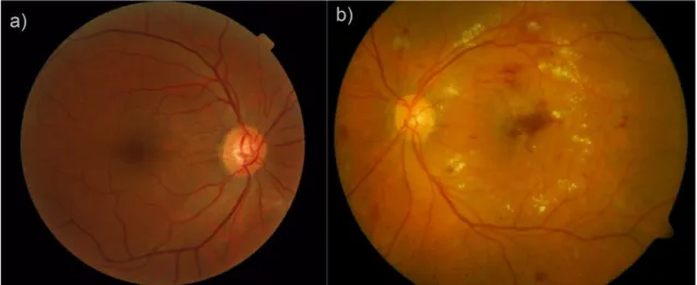
Diabetic retinopathy is a complication of diabetes and it is a vascular disease of the retina (Figure 1b). It is caused by the long-term effects of high glucose levels on the microvas-cular system. Diabetic retinopathy is one of the considerable causes of visual impairment and blindness globally (World Health Organization 2016). The early detection of diabetic retinopathy with proper guidance can lower the risk of severe vision loss by 90 % (Garg & Davis 2009). Sometimes the patient is not even aware of the fact that he has diabetes especially in the case of type 2 diabetes.
Figure 1. (a) A healthy retina and (b) a retina with the signs of diabetic retinopathy
To detect, diagnose and follow the development of diabetic retinopathy and other ocular diseases, non-invasive retinal imaging can be used. Retinal imaging is an optic imaging method. Ophthalmologists and other qualified medical experts analyze the retinal images. The process of analysis is subjective, time consuming and laborious. While the prevalence of diabetes and obesity (that is linked to type 2 diabetes) keep increasing, also the number
of retinal images that need analysis is increasing. The answer to these challenges could be found in medical image analysis and computer-aided detection.
Medical image analysis aims to classify various tissue types based on the question at hand and it has been applied for example to magnetic resonance imaging (MRI), computed tomography (CT) and X-ray imaging. Computer-aided detection systems help medical experts to detect tumors or lesions and to do that, these systems can use artificial intelli-gence and computer vision with image processing methods. For example, medical image analysis and computer vision have been applied to the quantitative analysis of the MRI images of the brain and thigh muscles (Sikiö 2016), the assessment of breast cancer in MRI images (Ahmed et al. 2013), the classification of gastroenterology images (Riaz et al. 2012) and the automated detection of tuberculosis in chest X-rays (Jaeger et al. 2014). The aim of this thesis was to design and implement a computer-aided detection system for diabetic retinopathy and lesions. The purpose was to study whether texture features are able to produce descriptive and efficient information for the retinal image classifica-tion. In addition, how accurate the implemented system would be for the detection of a diabetic retinopathy and related lesions.
The implemented system had high accuracy, sensitivity and specificity in red lesion de-tection. The selected texture features were able to produce efficient and descriptive infor-mation on a local setting. This system could help ophthalmologists and other experts in their clinical workflow by lowering manual labor and making the analysis more accurate, precise and efficient. In addition, this could enable an early detection of diabetic retinopa-thy and therefore improve the quality of life of diabetics.
This thesis was part of a TEKES funded project at University of Oulu. The aim of the project was to map out research possibilities by combining data analysis and ophthalmic health. Researcher Riku Hietaniemi from University of Oulu was guiding the represented implementation.
The thesis is divided into six chapters. Chapter 2 describes the basics of diabetes, diabetic retinopathy and retinal imaging. Chapter 3 introduces medical image analysis. First the subject is issued generally and then related to the retinal images. Chapter 4 presents the information about the methods used in this thesis and Chapter 5 describes the experiments and the results with discussion. Chapter 6 contains the conclusion of this thesis. Appendix A includes the equations of the gray level co-occurrence matrix related statistical param-eters.
2. DIABETES AND RETINAL IMAGING
The retina is an interior tissue layer in the eye. When incoming light travels to the eye, the retina enables the conversion of light into nerve impulses and these impulses are con-verted into images in our brains. Diseases and complications, such as diabetes or cardio-vascular diseases, affect the health of the retina. Diabetic retinopathy is a complication of diabetes mellitus and it is one of the considerable causes of visual impairment and blind-ness globally (Pascolini & Mariotti 2012). Retinal imaging is used to analyze ocular struc-tures, evaluate the health of the retina and to detect and diagnose possible diseases such as diabetic retinopathy. Retinal images are also used in follow-up to diseases and treat-ments.
2.1 Diabetes
Diabetes mellitus is a metabolic disorder that is characterized by high blood sugar (hy-perglycemia). To control high glucose levels in blood stream, beta cells in pancreatic islets produce and secrete insulin hormone. Insulin increases the uptake and utilization of glucose into cells and as a result the concentration of glucose in blood stream starts to decline into normal (70–110 mg/dl). If the insulin production is inadequate, the blood glucose levels stay high and excess glucose is released into urine. On the other hand, body can become resistant to insulin if its concentration in blood stream is continuously high. (Martini 2006)
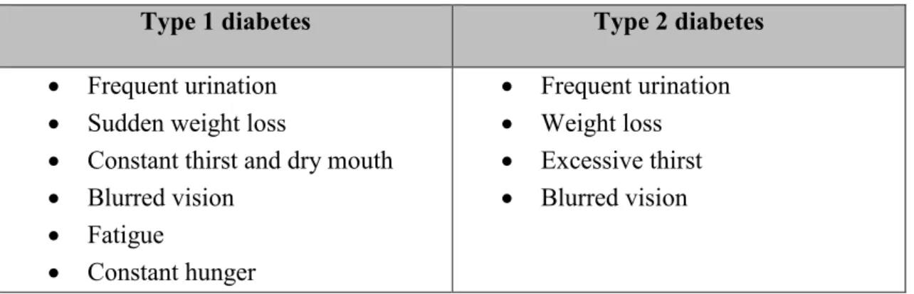
Diabetes has been classified into four main categories: type 1, type 2, gestational and other. Type 1 diabetes is an autoimmune disease of the pancreas and it usually advances quite slowly. In the end, it leads into insulin deficiency and Type 1 diabetic is dependent on insulin in a form of a replacement hormone. The type 2 diabetes is caused by insulin resistance and dysfunctional insulin secretion. It can be hard for a person to notice that they have the symptoms of type 2 diabetes (Table 1) since the disease is linked with other medical problems such as central obesity, high blood pressure and unbalanced cholesterol levels. These are significant cardiovascular risk factors. Management of the type 2 diabe-tes includes healthy lifestyle and medication. Gestational diabediabe-tes develops during preg-nancy and the last category includes less common types of diabetes. (Leu & Zonszein 2010)
Table 1. Symptoms of type 1 and type 2 diabetes
Type 1 diabetes Type 2 diabetes
• Frequent urination • Sudden weight loss
• Constant thirst and dry mouth • Blurred vision • Fatigue • Constant hunger • Frequent urination • Weight loss • Excessive thirst • Blurred vision
There is a strong link between cardiovascular diseases and diabetes. Vascular tissues suf-fer from high levels of glucose in the blood stream due to the resulting biochemical reac-tions. These reactions affect the inner cells and muscle cells of vessels. One major path-way to vessel damage is glycosylation. When glucose is circulating in blood stream, it can unintentionally attach to protein molecules and affect their normal functioning. Man-aging the blood glucose levels is challenging. Cardiovascular problems and microvascu-lar complication arise from poorly managed blood glucose control. They lead for example into foot ulcers and amputation, kidney failure and vision loss. Cardiovascular disease is the most probable cause of death of type 2 diabetics. (Devereux 2010; Laud & Shabto 2010; Leu & Zonszein 2010)
2.2 Retina
The retina is the inner layer of the eye (Figure 2). The retina itself has two layers called the pigmented part and the neural part. The neural part senses the light that enters the eye and the pigmented part absorbs it. The light creates biochemical reactions in retina’s pho-toreceptors and then, nerve impulses are sent through the optic nerve and visual pathway into the visual cortex of the brain. This part of the brain then forms images i.e. our vision. (Martini 2006)
The major blood vessels of the retina are radiating from the center of the optic nerve. The beginning of the optic nerve in the retina is called the optic disc. This part is also known as the blind spot since there are no photoreceptors. The spot with the highest concentra-tion of cone photoreceptors is called fovea, the area of clear vision. The cone photorecep-tors are responsible for giving clear vision in full colors. Macula (or macula lutea) is the area around the fovea. (Martini 2006)
Figure 2. Anatomy of the retina (Kolb 1995)
2.3 Diabetic retinopathy
A person with diabetes mellitus can develop diabetic retinopathy, which is a vascular disorder of the retina. Probability to develop diabetic retinopathy gradually increases over the years. It is easier to calculate a time domain for type 1 diabetic since the onset of type 2 diabetes is usually quite uncertain. Another risk factor is blood glucose control, which affects capillaries. Regular follow-ups are important. (Laud & Shabto 2010)
The rupture, degeneration and excessive growth of blood vessels invade the space be-tween the neural layer and pigmented layer. Visual acuity is threatened by a leakage of blood, new blood vessels and damage of photoreceptors. There is no cure but healthy lifestyle can help to prevent the progress and temporary fixes such as laser therapy are an option. (Martini 2006; Laud & Shabto 2010)
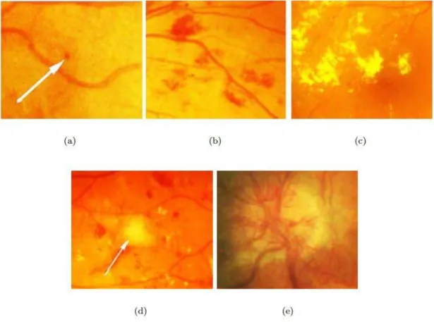
Microaneurysms are the earliest clinical signs of diabetic retinopathy (Figure 3a). Micro-aneurysms are located in retinal capillaries in any part of the retina and they appear as round and small red dots. The number of microaneurysms can predict the progression of retinopathy if they are increasing, decreasing or if the amount stays the same. The in-creasing number of microaneurysms indicate the progression of the disease. Hemor-rhages have variety in their shape and size (Figure 3b). Very small hemorHemor-rhages can be hard to distinguish from microaneurysms while larger hemorrhages can resemble blots. Hemorrhages form when microaneurysm or weak vascular wall breaks within the retina. Microaneurysms and hemorrhages are also referred to as red lesions. (Chen 2008; Laud & Shabto 2010)
Exudates are also connected to diabetic retinopathy. Hard exudates are leaked lipopro-teins and appear as white or yellow (Figure 3c). These exudates have strict outlines. Soft exudates are called cotton wool spots due to their soft shape (Figure 3d). Soft exudates arise from the nerve fiber layer where axoplasm is leaking. Hard exudates and cotton wool spots are also referred to as bright lesions. (Chen 2008)
When diabetic retinopathy progresses into a more severe state, the signs of abnormal growth of blood vessels start to surface. Intraretinal microvascular abnormalities (IRMA) form loops of vessels that splay other vessels. Neovascularization can lead into leaking vessels, sudden vision loss or even retinal detachment (Figure 3e). In venous beading, a vessel has both thinning and dilating parts. (Laud & Shabto 2010)
Figure 3. Symptoms of diabetic retinopathy. (a) A microaneurysm, (b) hemorrhages, (c) hard exudates, (d) soft exudate and (e) neovascularization in the optic disc. (Kauppi 2010)
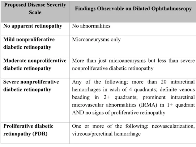
The abnormalities in the retina can define two categories: nonproliferative diabetic reti-nopathy (NPDR) or proliferative diabetic retireti-nopathy (PDR). NPDR is also known as background retinopathy. Lesions that are associated with NPDR are microaneurysms, hemorrhages, cotton wool spots and hard exudates. NPDR has three stages and it can advance into PDR with the abnormal growth of blood vessels. Table 2 represents connec-tions between the findings and severity of retinopathy. (Laud & Shabto 2010)
Table 2. Diabetic Retinopathy Disease Severity Scale (Wilkinson et al. 2003)
Proposed Disease Severity
Scale Findings Observable on Dilated Ophthalmoscopy No apparent retinopathy No abnormalities
Mild nonproliferative diabetic retinopathy
Microaneurysms only
Moderate nonproliferative diabetic retinopathy
More than just microaneurysms but less than severe nonproliferative diabetic retinopathy
Severe nonproliferative
diabetic retinopathy Any of the following; more than 20 intraretinal hemorrhages in each of 4 quadrants; definite venous beading in 2+ quadrants; prominent intraretinal microvascular abnormalities (IRMA) in 1+ quadrant AND no signs of proliferative retinopathy
Proliferative diabetic
retinopathy (PDR) One or more of the following: neovascularization, vitreous/preretinal hemorrhage
Diabetic macular edema is sight threatening condition where retinal lesions are located near the center of the macula. In the severe stage, hard exudates have reached the center. Macular edema can include thickening of the retina or hard exudates. In NPDR, the mac-ular edema is the primary reason for visual loss. (Wilkinson et al. 2003; Chen 2008; Laud & Shabto 2010)
2.4 Retinal image acquisition
Fundus photography is an optical method and therefore it is based on reflected light, which projects the retinal tissues to a two-dimensional (2D) representation. Fundus im-aging is used to detect for example age-related degeneration and diabetic retinopathy. An expert makes the evaluation of the retina based on subjective analysis of colors, structures and shapes. (Abràmoff et al. 2010; Kaschke et al. 2013)
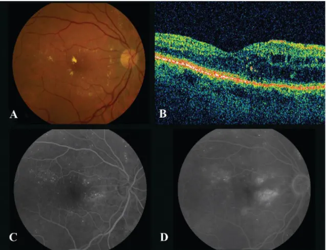
Fundus photography has a wide category of different modes. A typical mode is color fundus photography (Figure 4a), which is performed with white light. By filtering the light, user can highlight specific retinal structures. When a green filter is used, retinal blood vessels have higher contrast in a red-free image. Fluorescein angiography is used to detect retinal vessels, blood circulation and leakages (Figure 4c and 4d). First, sodium fluorescein dye is injected into a vein and then a series of images is obtained to detect the
circulation of the dye. Unfortunately, the dye can cause side effects such as nausea, vom-iting, rash or even severe reactions. Stereo imaging mode produces a pair of monocular images that provide a stereoscopic view of for example optic nerve. (Abràmoff et al. 2010; Laud & Shabto 2010; Kaschke et al. 2013)
Optical coherence tomography (OCT) provides information about layered retinal struc-tures and its histological changes (Figure 4b). It is based on a measurement of distance and time of flight of backscattering light. The wavelength of the light used is usually longer than visible light’s wavelength. To get a 2D image, the beam of light moves in depth (z-axis) across the retina in transverse (x-axis) direction. The three-dimensional (3D) image is formed by stacking the 2D images at orthogonal positions (y-axis). The thickness and volume of the retina can be measured with OCT and therefore it is optimal to detect macular edema, macular degeneration, glaucoma and inflammatory diseases. (Abràmoff et al. 2010; Kaschke et al. 2013)
Figure 4. Retinal images. (A) Color fundus photography, (B) OCT: Optical coherence tomography and (C–D) Fluorescein angiogram (Meyerle et al. 2008)
2.5 Quality of retinal images
The homogeneity and good quality of retinal images decreases complexity and eases the analysis for humans and for computers. However, retinal imaging is technically challeng-ing operation and images can include artefacts and wide technical variation due to users, patients or devices. In the worst case, the image cannot be evaluated.
There are several challenges in the retinal imaging. The smallest objects are in microme-ters. Access to the retina is challenging since the light travels through a small hole i.e. through the pupil. The patient has to stay still since even a small shift in position affects the result. Some objects and structures have low contrast and need to be enhanced for example with fluorescein dye. When a 3D object is photographed and 2D image is pro-duced, information gets lost. The curved shape of the fundus is also a challenge for the imaging. (Kaschke et al. 2013)
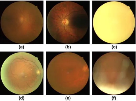
Artefacts can significantly affect the image quality. Figure 5 represents retinal images with poor quality. Typical artefacts are smudges on the lens, light artefact and non-uni-form illumination. Small pupils, eye diseases and certain conditions that increase opacity can block or limit the light that enters the eye, which can therefore lower the sharpness of the image and create non-uniform illumination. This can create blurred or dark images. The color of the retina has variation due to age or ethnicity, which can create challenges to the assessment of the image. (Dias et al. 2014)
Figure 5. Retinal images with poor quality. (a) Poor focus, (b) Uneven illumination, (c) Blinked eye, (d) Light artefact, (e) Dust and dirt (near the center) and (f) eyelash artefact. (Dias et al. 2014)
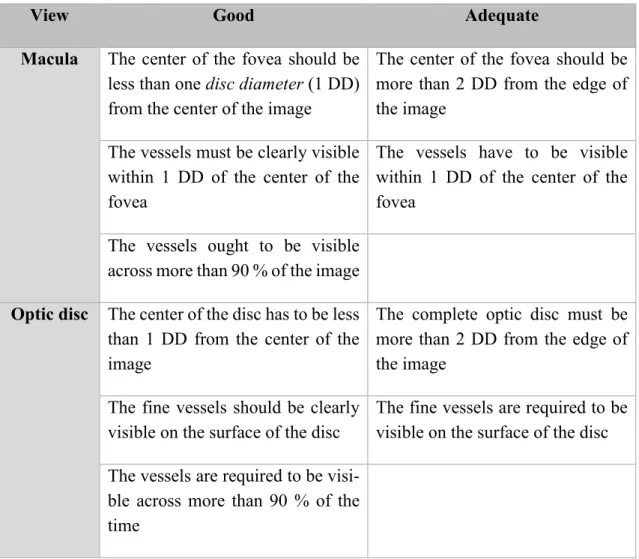
Retinal imaging instruments from different manufactures have different settings and char-acteristics. The devices can have different Field of Views (FOV) and resolutions. Typical FOV is 50 degrees. Depending on the user of the device and purpose of the image, the images can have different views of focus (macula or optic disc). (Kaschke et al. 2013) An ideal retinal image is free of reflections, artefacts and is uniformly illuminated. The image has high sharpness, FOV, contrast, resolution and the details are clearly visible. Table 3 describes informal quality specifications for technically satisfactory images from macula and optic disc view. The disc diameter (DD) is the diameter of the optic disc. The positioning of the image is important for the detection of abnormalities. (Taylor & Batey 2012; Kaschke et al. 2013)
Table 3. Definitions for technically satisfactory image (Taylor & Batey 2012)
View Good Adequate
Macula The center of the fovea should be less than one disc diameter (1 DD) from the center of the image
The center of the fovea should be more than 2 DD from the edge of the image
The vessels must be clearly visible within 1 DD of the center of the fovea
The vessels have to be visible within 1 DD of the center of the fovea
The vessels ought to be visible across more than 90 % of the image
Optic disc The center of the disc has to be less than 1 DD from the center of the image
The complete optic disc must be more than 2 DD from the edge of the image
The fine vessels should be clearly visible on the surface of the disc
The fine vessels are required to be visible on the surface of the disc The vessels are required to be
visi-ble across more than 90 % of the time
2.6 Diabetic retinopathy datasets
There are several retinal image databases available online related to diabetic retinopathy. Seven image sets that are related to the detection of abnormalities or classification of diabetic retinopathy are introduced in the following subchapters.
2.6.1 Messidor
Messidor is an abbreviation of “Methods for Evaluating Segmentation and Indexing tech-niques Dedicated to Retinal Ophthalmology”. Messidor dataset has 1 200 images where 546 images are classified as healthy and 645 images are classified as retinopathy. The images were acquired in three ophthalmologic departments with a Topcon TRC NW6 fundus camera before the year 2007. The field of view is 45 degrees and image sizes are 1440*960, 2240*1488 and 2304*1536 pixels. (MESSIDOR 2016)
The classification is divided into healthy (as class 0) and three stages of retinopathy se-verity (classes 1–3) based on microaneurysm, hemorrhage and neovascularization find-ings (Table 4). The images are classified based on retinal lesions but the locations and exact amounts of lesions are not reported. In addition, a risk factor for macular edema is reported with three classes. Class 0 represents absent risk for macular edema and classes 1–2 are at risk. The ground truths are provided as an Excel file. (MESSIDOR 2016)
Table 4. Retinopathy grade in Messidor database based on findings (MESSIDOR 2016)
Retinopathy grade Findings
Class 0 No microaneurysms AND no hemorrhages
Class 1 Amount of microaneurysms is 1–5 AND no hemorrhages Class 2 Amount of microaneurysms is 6–15 OR amount of hemorrhages
is 1–4 AND no neovascularization
Class 3 Amount of microaneurysms is greater than 15 OR amount of hemorrhages is greater than 4 OR neovascularization is present
2.6.2 DIARETDB
As a subproject for the Imageret project, Kauppi et al. (2007) created two standard dia-betic retinopathy datasets called DIARETDB0 and DIARETDB1. DIARETDB0 dataset has 130 images where 20 images have no signs of retinopathy and 110 images have at least mild NPDR signs. DIARETDB1 dataset has 89 images where 5 images have no signs of retinopathy and 84 images have at least mild NPDR signs. (Kauppi et al. 2007) All the images were acquired in Kuopio University hospital before the year 2007. The DIARETDB1 set is acquired with one fundus camera while DIARETDB0 set has images by several fundus cameras. The field of view is 50 degrees and image size is 1500*1152 pixels. (Kauppi et al. 2007)
Four experts have annotated the images and marked hard and soft exudates, microaneu-rysms and hemorrhages. They were instructed to use shapes of centroid, polygon, circle and ellipse with a representative point in the middle of the shape. The experts also re-ported their confidence level considering the findings. The severity of diabetic retinopa-thy is not reported. The annotations are provided as XML files that include types, coor-dinates, confidence levels and shapes. (Kauppi et al. 2007)
2.6.3 Retinopathy Online Challenge (ROC)
Meindert Niemeijer, Michael D. Abramoff and Bram Van Ginneken organized the Reti-nopathy Online Challenge (ROC), which was an international competition for microan-eurysm detection. They provided color fundus images divided as 50 training images and 50 test images. The training set included reference standard of microaneurysms and dot hemorrhages. The competition started February 2008. At the moment, the submissions are not possible but the files are available by download. (Niemeijer et al. 2010)
The images were selected from a larger set of 150 000 images and were acquired in dif-ferent places. The images were acquired with either a Canon CR5-45NM, a Topcon NW 100 or a Topcon NW 200 camera. There are two image shapes present due to the different types of cameras. The coverage of the retina is 45 degrees and image sizes are 769*576, 1058*1061 and 1389*1383 pixels. (Niemeijer et al. 2010)
Four experts have annotated the images. They were asked to mark the center locations of microaneurysms and other lesions that look similar such as hemorrhages and pigment spots. Only the microaneurysms were included in the reference standard but in the com-petition, detecting similar lesions were not counted as a false positive. The annotations are provided as a XML file that includes coordinates and radii. (Niemeijer et al. 2010)
2.6.4 E-ophta
The e-ophta is a color fundus image database that is extracted from the Ophdiat project. Ophdiat was a five-year telemedicine screening program for diabetic retinopathy in France. The Ophdiat project started in 2004 and in total 51 741 examinations were made. (Schulze-Döbold et al. 2012; Decencière et al. 2013)
The e-ophta database is divided into e-ophta EX and e-ophta MA subsets. The e-ophta EX includes 35 healthy images and 12 278 annotated exudates within 47 images. The e-ophta MA set includes 233 images free of microaneurysms and 1 306 annotated micro-aneurysms and other small red lesion within 148 images. (Decencière et al. 2013) The e-ophta images were acquired between the years of 2008 and 2009 in different places either with a Canon CR-DGi or with a Topcon TRC-NW6 camera. The coverage of the retina is 45 degrees and image sizes are 1440*960, 2048*1360 and 2544*1696 pixels.
The annotations are provided in a form of binary masks corresponding to the positions of microaneurysms or exudates in the original images. (Schulze-Döbold et al. 2012; De-cencière et al. 2013)
2.6.5 Kaggle competition
Kaggle website runs machine learning related programming contest. Kaggle had a ma-chine learning competition for diabetic retinopathy detection in 2015. The competition was popular since 661 teams and 854 contestants participated in it. The competition da-taset had almost 90 000 images. The dada-taset has lots of variation since its purpose is to mimic real situation. (Kaggle 2015)
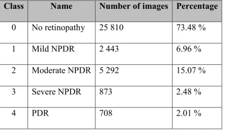
The training set included 35 126 images with ground truth, the test set included 53 576 images and both eyes of a patient were presented. The stage of diabetic retinopathy was marked by an expert. As presented on the Table 5, there is a scale from zero to four: no signs of diabetic retinopathy (class 0), mild (class 1), moderate (class 2), severe (class 3) and proliferative diabetic retinopathy (class 4). (Kaggle 2015)
Table 5. Kaggle training set images (Kaggle 2015)
Class Name Number of images Percentage
0 No retinopathy 25 810 73.48 %
1 Mild NPDR 2 443 6.96 %
2 Moderate NPDR 5 292 15.07 %
3 Severe NPDR 873 2.48 %
4 PDR 708 2.01 %
The image acquiring methods, devices and conditions have lots of variation. Image sizes vary, but the images are on average 3000*2000 pixels, which is quite large. The images and labels include noise in a form of artefacts, underexposure, overexposure, out of focus images and outliers. (Kaggle 2015)
2.6.6 Diabetic Retinopathy Image Database (DRiDB)
Diabetic Retinopathy Image Database (DRiDB) was created by the image processing group in University of Zagreb, Croatia. The database contains 50 color fundus images. The images were acquired at the University Hospital of Zagreb with Zeiss Visucam 200 camera. The coverage of the retina is 45 degrees and image size is 720*576 pixels. The
set has 36 images that contain diabetic retinopathy signs and 14 images that do not contain any signs. (Prentašić et al. 2013)
The dataset contains annotations from several experts and at least five experts have an-notated one image. The experts marked all fundus structures, pathologies and grade of the disease. They were asked to mark hard exudates, soft exudates, microaneurysms, hem-orrhages, optic disc, macula, blood vessels and neovascularization. (Prentašić et al. 2013)
2.6.7 High resolution fundus (HRF)
The high resolution fundus (HRF) image database was a result of a collaborative research project by the University of Erlangen-Nuremberg, Germany and Brno University of Tech-nology, Czech Republic. The image database includes 15 images of diabetic retinopathy and 15 images of healthy eyes. Diabetic retinopathy images include hemorrhages, neo-vascularization, bright lesions and laser treatment spots. Experts have labeled the blood vessels of the images. The dataset is mainly intended for the research of automated vessel segmentation but it is also valid for classification. The images were acquired with a Canon CF-60UVi camera and the image size is 3504*2336 pixels. The coverage of the retina is 60 degrees. (Odstrcilik et al. 2013)
3. MEDICAL IMAGE ANALYSIS
The human eye was described shortly in Chapter 2.2. First, we receive an image through our eyes, then it is transmitted through the nervous system and finally, it is processed and analyzed by our brain. A computer vision system acquires its images by a camera. Images can be defined as of a two-dimensional function f(x,y) with spatial coordinates x and y. The value of f is the gray level or color at a certain point (x,y) of the image. These points are called pixels and an image can be stored as an array of values I[x,y]. Algorithms that extract quantitative information are used to process and analyze images. The aim of the system is either to make a decision about the content of the image or to classify containing objects. (Shapiro & Stockman 2001; Nixon & Aguado 2012)
Generally, medical image analysis has four steps: preprocessing, region extracting, fea-ture engineering and classification. The purpose of the preprocessing steps is to reduce noise, clear artefacts, enhance image quality and normalize images. Normalization is an important step for example when illumination conditions vary with images. Analyzing medical images also includes detecting different regions. Those regions can be extracted for better visualization and careful analysis. To better analyze the regions, quantitative measurements of the interest regions can be conducted. As a result, feature vectors are created. Finally, these regions can be analyzed and classified accordingly. In supervised learning, the outputs are known for the training samples and a classifier can be trained guided by that knowledge of outputs with the feature vectors as inputs. In medical image analysis, the known outputs are the ground truths made by medical experts. The results of the classifier are compared with the ground truths of the validation samples to deter-mine the performance of the classifier. The topics are presented in the consideration of this study and its methods. (Shapiro & Stockman 2001)
3.1 Image preprocessing
Image preprocessing is an important step in image analysis. In digital images, pixels are finite and discrete values and images can be presented with standardized color models (Gonzalez & Woods 2002). To make the images more uniform color wise, image en-hancement and normalization can be applied. Some image analysis applications need seg-mentation of objects or areas and this can be done with the help of binary operations.
3.1.1 Color models
A color model or color space describes and specifies colors in a standardized and com-monly accepted way. Colors are bind to a coordinate system where a single point repre-sents a certain color. Common color models in image processing are RGB, CMY and HSV models. (Gonzalez & Woods 2002)
A well-known color model is the RGB model. RGB stands for red, green and blue. This model is hardware oriented and it is most commonly used in color monitors. When an image is presented in the RGB color space, it is a combination of three component images. In Figure 6a there is a RGB image and Figures 6b, 6c and 6d represent the R, G and B component images. In the component images, the pixel value 0 represents black and pixel value 255 represents white when the pixel depth is 8 bits per channel and in total 24 bits. A 24-bit RGB image can have 16 777 216 colors but in the end only a few hundred colors are used in everyday applications. (Gonzalez & Woods 2002)
Figure 6. (a) RGB image and (b–d) three color channels
The CMY and the CMYK color models are hardware oriented and they are used in color printing. The letters stand for cyan, magenta, yellow and black. These colors (excluding black) are the primary colors of the pigments and secondary colors of light. The CMY model also uses three component images. The relationship between RGB and CMY is expressed as [ 𝐶 𝑀 𝑌 ] = [ 1 1 1 ] − [ 𝑅/255 𝐺/255 𝐵/255 ] , (1)
where R, G and B are first normalized to scale between zero and one. Resulting C, M and Y are also in the scale between zero and one. Black is added as fourth color in the CMYK model since it is a predominant color in printing. In theory, mixing equal amounts of cyan, magenta and yellow produces black, but for the printing purposes, this method is not functional. (Gonzalez & Woods 2002)
Another color model is the HSV model, which has been developed from HSI model that resembles the way that humans interpret and describe colors. The HSV stands for hue, saturation and value. The hue describes a pure color, the saturation corresponds to the
dissolved white light and the value describes brightness or intensity. The relationship be-tween RGB and HSV is 𝐻 = { 𝜃, 𝐵 ≤ 𝐺 360 − 𝜃, 𝐵 > 𝐺 , 𝑤ℎ𝑒𝑟𝑒 𝜃 = cos−1{ 1 2[(𝑅 − 𝐺) + (𝑅 − 𝐵)] [(𝑅 − 𝐺)2+ (𝑅 − 𝐵)(𝐺 − 𝐵)]1/2} , (2) 𝑆 = 1 −min(𝑅, 𝐺, 𝐵) max(𝑅, 𝐺, 𝐵) , (3) 𝑉 = max(𝑅, 𝐺, 𝐵) , (4)
where H and θ are given as an angle that rotates counterclockwise. The HSV color space is advantageous for grayscale techniques since it separates grayscale and color infor-mation in an image. (Gonzalez & Woods 2002)
3.1.2 Contrast enhancement and color normalization
Contrast is the difference in luminance or color. If an image has low dynamic range of gray levels, the contrast is low. A simple method in order to get higher contrast is contrast stretching where the range of gray levels, between black and white, is broadened. Histo-gram represents the distribution of gray level values in an image. When the values are spread through the histogram, the result is fuller gray scale range. This method is called histogram equalization. (Gonzalez & Woods 2002)
Contrast-limited adaptive histogram equalization (CLAHE) is an advanced local contrast enhancement method. The method processes small tiles of an image and combines the results with bilinear interpolation to avoid local boundaries. In the beginning, a clip limit is set for the histogram of a gray level image depending on histogram normalization and neighborhood size. The output value for a single pixel is its rank in the local histogram. A part that exceeds the clip limit is redistributed to other bins and the clip limit is modi-fied. The procedure can be repeated recursively if the results are not satisfactory. (Pizer et al. 1990)
When images that are compared come from multiple subjects, normalization may be needed for successful comparison. Here, normalization refers to the mapping of the colors of different images into a common norm. Varying illumination creates the distribution of color values in an image. Color normalization can be performed with image enhancement techniques such as histogram equalization, histogram specification or color channel
length normalization. In the histogram specification, the histograms are matched to a ref-erence histogram. In color channel length normalization, the pixels are normalized first and then each color channel. (Goatman et al. 2003; Toennies 2012)
3.1.3 Segmentation and binary operations
In image segmentation, an image is subdivided into regions or objects for example into a background and an object in the image. Algorithms in image segmentation are generally divided into two basic styles: algorithms that make the partition based on sudden changes in intensity (edges) or based on regions that share certain criteria. A fundamental ap-proach in both categories is the thresholding method. (Gonzalez & Woods 2002)
In its simplest form, global thresholding creates a binary image from an original grayscale image by a mathematical operation with a set threshold level. Thresholding turns all pix-els that are below the given threshold level to zero (representing background points) and other pixels to one. The binary image can be used as a mask when segmenting areas or objects from the original image. The pixels of the original image are multiplied by the corresponding binary value of the binary mask. The pixels that were classified as object points stay unchanged while the pixels classified as background points are set to zero. (Gonzalez & Woods 2002)
Thresholding is effective when an image has a high level of contrast. The problem with the method is that it only considers intensities of pixels but not their relationships. It can be also sensitive to uneven illumination or noise. The threshold level can also change over an image and it could be adapted for example with the help of a histogram. To solve the uneven illumination, an adaptive thresholding method can be used using local properties. (Gonzalez & Woods 2002)
If the binary mask was created by thresholding, it may need some preprocessing for ex-ample with morphological methods before applying it to the original image. Two basic operations of morphology are erosion and dilation, where a structuring element is used to either enlarge or scale down a region (Figure 7). The structuring element is a neighbor-hood of binary pixels and it represents a shape in any size and chosen structure. Common shapes are a rectangle and circular shape, but also for example square, diamond, disk or octagon shapes could be used. (Shapiro & Stockman 2001; Gonzalez & Woods 2002)
Figure 7. Morphological operations with the structuring element (se)
In Figure 7, the original object is processed with a square structuring element “se”. The center point of the structuring element is traveling through the edges of the original object. In the erosion operation, the structuring element has traveled through the dotted line, studied the local neighborhood and erased object pixels where needed. The dilation oper-ation follows same protocol but instead of erasing object pixels, the structuring element adds pixels. (Shapiro & Stockman 2001; Gonzalez & Woods 2002)
3.2 Feature extraction and texture features
Feature extraction is used to extract relevant information from images. To quantify the information, the properties of image texture can be used. A texture feature is in a form of feature vector, which includes a set of measurements from images.
Structure or a surface of an object has properties described as textures. For humans, the concept of texture seems obvious but it is quite challenging to define it. Whereas in digital images, a group of pixels in different tones, scales and structures represent different tex-tures. One pixel alone cannot define texture. Image textures have information about amount and type of texture areas (primitives) and their spatial relationships. (Tuceryan & Jain 1998)
In computer vision, recognition and classification of textures are useful and important part of a process. Texture has been used for example in recognition of objects, shape analysis and image segmentation. A general challenge in computer vision is the shape of a target. Texture can give more information about the shape and surface orientation of an object. Texture segmentation tries to identify texture boundaries even though the actual textures are unknown. (Tuceryan & Jain 1998)
Textures can be described for example as coarse or fine. When texture elements are large and include several pixels, the texture is coarse. The texture is fine when the elements are small and neighboring pixels clearly differ in tone. (Sonka et al. 2008) Other possible properties to describe textures are a direction, directionality, frequency, a phase, density,
roughness, coarseness, regularity, uniformity and linearity. Some of the properties are dependent on each other. (Tuceryan & Jain 1998)
A geometrical method in texture analysis is based on the idea of texture primitives and structural approach assumes that texture has repeated or regular relationships between tones or structures. Textures do not always have geometrical regularity and cannot ade-quately be described by shapes. With statistical texture description methods, different statistical properties are computed from an image texture based on the gray level spatial distribution. It is suitable for images where pixel size and a texture primitive are compa-rable. Model based methods try to interpret a texture by generative image models and are more common in synthetic texture generation. (Tuceryan & Jain 1998; Sonka et al. 2008) A texture feature is in a form of feature vector, which includes a set of measurements. A good feature vector assigns the texture to some specific class. First-order histogram fea-tures, gray level co-occurrence matrix, local binary pattern, Gabor filter and Laws’ texture energy measures are all methods to extract texture features from images.
3.2.1 First-order histogram features
Variance, skewness and kurtosis are first-order features. These features are calculated using intensity histograms. When a histogram is used, variance measures the dispersion of the region intensity, skewness estimates the degree of asymmetry and kurtosis de-scribes peaks in the histogram. (Batchelor & Whelan 2012) The equations are
𝑉𝑎𝑟𝑖𝑎𝑛𝑐𝑒: 𝜎2 = ∑(𝑖 − 𝜇)2 ℎ(𝑖) 𝐴−1 𝑖=0 , (5) 𝑆𝑘𝑒𝑤𝑛𝑒𝑠𝑠: 𝜇3 = 𝜎−3∑(𝑖 − 𝜇)3 ℎ(𝑖) 𝐴−1 𝑖=0 , (6) 𝐾𝑢𝑟𝑡𝑜𝑠𝑖𝑠: 𝜇4 = 𝜎−4∑(𝑖 − 𝜇)4 ℎ(𝑖) 𝐴−1 𝑖=0 , (7)
where i is a gray level value, A is the amount of gray levels in an image, h is the histogram, σ is standard deviation and μ is mean. These features can be used to describe texture but they lack information about the spatial relationships of pixels. (Batchelor & Whelan 2012)
3.2.2 Gray Level Co-occurrence Matrix (GLCM)
Gray level co-occurrence matrix (GLCM) is a statistical texture description method. It is based on a repeated occurrence of gray level structures in an image. The image can be quantized into a number of gray levels to limit the size of the resulting matrix. Co-occur-rence matrix CM includes frequencies of two pixels’ occurCo-occur-rence. It indicates how many times the reference gray level value i occurs with the neighbor gray level value j in the certain spatial relationship in an image I (Figure 8). The GLCM can be computed in the following way: 𝑪𝑴(𝑖, 𝑗) = ∑ ∑ { 1, if 𝐼(𝑝, 𝑞) = 𝑖 and 𝐼(𝑝 + ∆𝑥, 𝑞 + ∆𝑦) = 𝑗 0, otherwise 𝐸 𝑞=1 𝐷 𝑝=1 (8)
where D and E indicate the size of an image I, ∆x is displacement in rows and ∆y is displacement in columns. The displacement can be also presented as an angle and a dis-tance where horizontal is 0 degrees. The size of the matrix CM is the number of gray values to the power of two. Processing an image takes the number of operations that are proportional to an image size (to D and E). Size of the matrix can be reduced by counting mirrored gray level pairs together for example by adding up pair I(1,2) and I(2,1). (Haralick & Shanmugam 1973; Shapiro & Stockman 2001; Batchelor & Whelan 2012)
Figure 8. Creation of GLCM in horizontal direction (0°). Adapted from (Sikiö 2016).
Rapidly changing co-occurrence distribution within a distance indicates a fine texture. While GLCM gathers properties of this kind from a texture, it is not that useful in the resulting form for comparing textures. Several, more compact statistical parameters can
be calculated from the co-occurrence matrix such as energy, contrast, homogeneity, en-tropy, autocorrelation, dissimilarity, cluster shade, maximum probability, sum average, sum entropy, sum variance, difference variance, difference entropy and two information measure correlations. These parameters are presented in the Appendix A. Some of the Haralick texture parameters describe the nature and complexity of varying gray tone structures when others are related to more specific textural characteristics and organized structures. (Haralick & Shanmugam 1973; Shapiro & Stockman 2001) For example, en-ergy measures image uniformity, entropy measures the complexity and contrast measures the local variation of intensity (Batchelor & Whelan 2012).
3.2.3 Local Binary Patterns (LBP)
Local binary patterns (LBP) method combines structural and statistical methods. LPB is very simple and it is based on pixel thresholding. Each pixel is compared with its neigh-boring pixels if their intensity is greater. In the beginning, the center pixel was compared with the neighborhood of size 3x3 but LBP was further developed to use circular neigh-borhoods in different sizes (Figure 9). The use of bilinear interpolation allows any number of pixels and any radius to be set. The method stores the occurrences of different patterns in the particular neighborhood of each pixel in to a histogram. The image can be divided into cells that all have their own histogram. The histograms of the cells are then combined to form the feature vector. LBP has invariance in rotation and illumination. It is compu-tationally simple and therefore fast. (Ojala et al. 2002)
Figure 9. Creation of LBP. 1) The sample, 2) the calculated differences related to the center and 3) the threshold values. (Pietikäinen & Zhao 2009)
3.2.4 Gabor filters
The Gabor filter is a statistical method and originally it is a signal processing method. The Gaussian kernel function called the envelope is modulated by a plane wave that is complex and sinusoidal. The plane wave is called a carrier. A 2D Gabor filter GF in the spatial domain is defined as:
𝑮𝑭(𝑥, 𝑦) = 𝑓 2 𝜋𝛾𝜂∗ 𝑒𝑥𝑝 (−( 𝑓2 𝛾2𝑥′2+ 𝑓2 𝜂2𝑦′2)) 𝑒𝑥𝑝(𝑗2𝜋𝑓𝑥′) , (9) 𝑥′= 𝑥 cos 𝜃 + 𝑦 sin 𝜃 , (10) 𝑦′= −x sin 𝜃 + 𝑦 cos 𝜃 , (11)
where θ is the orientation of the surface normal to the parallel stripes, γ is the spatial aspect ratio (major), η is the spatial aspect ratio (minor) and f is the frequency of the sinusoid. The Gabor filters are convoluted with the original image. A Gabor filter is se-lective in frequency and orientation and it emphasizes edges and changing textures. For example, selecting eight orientations and five scales create 40 Gabor filters. The Gabor features are extracted from gray level images and further calculations can be conducted to get a compact presentation. (Petkov 1995; Haghighat et al. 2015) The method is robust against noise and illumination changes and it is invariant to translation, scale and rotation (Kamarainen et al. 2006).
3.2.5 Laws’ texture energy measures
Laws’ texture energy measures are based on local masks. Fixed-size windows are used for measuring the amount of variation within the window. Laws’ texture energy masks are named as Wave, Level, Ripple, Edge and Spot. (Laws 1979; Sonka et al. 2008) Laws (1979) defined the center-weighted vector masks as:
𝐿5 (𝐿𝑒𝑣𝑒𝑙) = [ 1 4 6 4 1] 𝐸5 (𝐸𝑑𝑔𝑒) = [−1 −2 0 2 1]
𝑆5 (𝑆𝑝𝑜𝑡) = [−1 0 2 0 −1] 𝑅5 (𝑅𝑖𝑝𝑝𝑙𝑒) = [ 1 −4 6 −4 1]
𝑊5 (𝑊𝑎𝑣𝑒) = [−1 2 0 −2 1]
The vectors are zero-sum (except Level), independent but not orthogonal. A set of 2D convolutional masks presented in Table 6 can be produced by taking the outer product of the 1D vectors. The product of E5 and L5 creates the mask E5L5. The Wave and its prod-ucts are not commonly used. To make the method invariant to rotation, some of the sym-metrical masks can be replaced with their average such as E5L5 and L5E5. The method can be made invariant to changes in contrast if the convoluted images are normalized with L5L5 mask. With filtering, the method can also be made invariant to luminance. (Laws 1979; Shapiro & Stockman 2001)
Table 6. Laws' energy maps
L5E5/E5L5 L5S5/S5L5 R5R5 R5W5/W5R5 E5W5/W5E5
L5R5/R5L5 E5E5 S5R5/R5S5 L5W5/W5L5 W5S5/S5W5
E5S5/S5E5 E5R5/R5E5 S5S5 W5W5
The basic algorithm of Laws is based on local energy. First, an image is filtered with a set of convolution masks to produce a set of filtered images. Then, the texture energy is measured for each pixel by processing the image with the local texture energy filter, which is a moving window average of the absolute valued pixels. Finally, statistics can be computed from the filtered image by for example calculating sum of squared pixel values that are normalized by the number of pixels. (Laws 1979)
3.3 Feature selection
Feature selection is used to find the informative and optimal combinations of features. When hundreds of features are used in classification, this increases dimensionality and makes the classification computationally intensive. Therefore, it is more efficient to find features that have the best class separability and cut out features that are less efficient. This can lead to data reduction, increased processing speed and improved performance of classification.
One of the categories in feature selection is filter methods, which rank individual features using a relevance index based on statistics or correlation coefficients. These methods are simple and practical, but ignore the classifier interaction. On the other hand, features can be more useful in a subgroup even though their individual properties are not that decisive. Wrapper methods study feature subsets and use a learning machine to score the subsets according to their predictive capabilities. Wrappers can be computationally intensive (de-pending on the learning machine) and have high risk of overfitting. Embedded methods are more specific to a selected learning machine and feature selection is performed under a learning process. Hybrid methods combine above mentioned methods. (Guyon & Elisseeff 2006)
3.4 Classification and evaluation
Classification is used to assign class labels for the samples. The class labels could be for example “normal” and “abnormal”. Classification is done based on the features and a sample can have a large number of features. When there is large amount of features, the dimensionality of feature space is also large. In supervised learning, the labels for the samples are already known. The classification has two steps: training and testing. Purpose
of the training step is to tune the classifier parameters based on the input and output con-nection. After the training step, the testing step assesses the performance of the classifier. The classifier can predict classes for new data. It is important that the samples in the training set and in the testing set belong only to one set. Otherwise the results are not proper. (Haykin 1999; Shapiro & Stockman 2001)
The classification is done with a classifier. Classifiers are algorithms based on mathemat-ical representations. There are several classifiers for two class problems and one of them is support vector machine (SVM). SVMs are feedforward networks that have hyperplanes as decision surfaces in a high dimensional feature space (Figure 10). When data is mapped into a higher dimensional space, it might be easier to separate the classes. SVMs aim to maximize the margin of separation between negative and positive samples. Support vec-tors are samples that the classifier has selected in the maximizing process and that are closest to the decision boundary. When the dataset is not separable, the aim is to minimize the probability of classification error. Adding a slack variable into the equation allows some of the point to be on the wrong side of the hyperplane. When the classes are not linearly separable, SVM can use kernels to create nonlinear decision surfaces. Such ker-nels are polynomial and radial-basis function (RBF). (Haykin 1999)
Figure 10. Support vector machine and the support vectors. Adapted from (Widodo & Yang 2007).
Another classifier is the k-nearest neighbors (kNN) algorithm. The classification is based on the distance of the nearest samples in the dimensional space. The assigned class for the new query instance is the majority vote of the classes of k-nearest instances. For ex-ample, in the Figure 11 the 5-nearest neighbor algorithm assigns the class for the new instance xq as negative based on the five nearest instances. (Mitchell 1997)
Figure 11. The query instance Xq would be assigned as negative with the 5-nearest neighbor (Mitchell 1997)
The classifier outputs are evaluated related to the ground truths. A ground truth for a sample is the correct class that has been assigned for example by a medical expert. If the ground truth and the test result both consider the sample as “abnormal”, this is considered as true positive (TP) while mutual consideration for “normal” is known as true negative (TN) (Figure 12). If the ground truth is “normal” for a sample but the classifier output is “abnormal”, it is considered as false positive (FP) and the opposite situation is false neg-ative (FN).
Figure 12. Relationships between ground truths and test results
With the outcomes of TP, TN, FP and FN, the classification accuracy can be measured along with the sensitivity and specificity as:
𝐴𝑐𝑐𝑢𝑟𝑎𝑐𝑦 = 𝑇𝑃 + 𝑇𝑁 𝑇𝑃 + 𝑇𝑁 + 𝐹𝑃 + 𝐹𝑁 , (12) 𝑆𝑒𝑛𝑠𝑖𝑡𝑖𝑣𝑖𝑡𝑦 = 𝑇𝑃 𝑇𝑃 + 𝐹𝑁 , (13) 𝑆𝑝𝑒𝑐𝑖𝑓𝑖𝑐𝑖𝑡𝑦 = 𝑇𝑁 𝑇𝑁 + 𝐹𝑃 . (14)
Accuracy, sensitivity and specificity are presented in percentages. The sensitivity presents how well the abnormal cases were classified correctly while the specificity presents this for the normal cases. If the specificity is high, it means that high percentage of the normal subjects are classified correctly as normal and only some samples are false alarms. The
receiver operating characteristic curve (ROC curve) method is used for classification method comparison. The curve plots the true positive rate against the false positive rate and the value of area under the curve (AUC) can be calculated from it.
The aim of the classifier is to classify the training samples accurately. A challenge arises when the training set is too small. This can lead to a tuned model that does not represent the data well enough. In overfitting, while the model is accurate on the training set, it performs worse with the test set. This can be the case also with noisy data. The ideal situation is that the classifier is designed so that it generalizes well for new data and it is accurate. (Mitchell 1997)
3.5 Analysis of retinal images
In this section, three methods for the retinal image analysis in the literature are presented. The literature is selected from the past five years based on their recognition. The methods are either used for red lesion detection or retinal image classification. Some methods are used for both purposes. Table 7 presents the summary of the results of the methods. Roychowdhury et al. (2014) created a computer-aided screening system for diabetic reti-nopathy, which was able to detect red and bright lesions from fundus images and generate a severity grade for NPDR. Their system was based on three stages: image segmentation, lesion classification and severity grading. Before the first stage, the images were prepro-cessed with histogram equalization, contrast enhancement and filtering. This was done to eliminate artifacts, blurriness and uneven illumination. In the first stage, red lesion can-didates and bright lesion cancan-didates were detected as two foregrounds while the optic disc and vasculature were detected as a background. The vasculature was detected using shade-correction and region growing method whereas the optic disc was detected using pixel intensity and location. The background objects were extracted since an optic disc can be mistaken as a bright lesion and vasculature as red lesions. The second stage clas-sified the red lesion and bright lesion candidates as non-lesions or true lesions. Then, the bright lesions were further classified as hard exudates or cotton wool spots and the red lesions were classified as microaneurysms or hemorrhages. They used 78 features includ-ing 14 structure-based features (area, orientation, solidity etc.), 16 features calculated from RGB and HSI color planes (minimum, maximum, mean and standard deviation) and 48 features using second-order derivative images. The structure-based features are pri-marily useful for classification between lesion and non-lesion. The features were scaled between 0–1. With feature selection and ranking process, they selected 30 features for classification. The used classifiers were Gaussian Mixture model for bright lesion detec-tion and kNN for red lesion detecdetec-tion. The third stage counted the lesions and assigned a diabetic retinopathy severity grade for an image. The system classified red lesions and non-lesions in DIARETDB1 set with sensitivity 80 % and specificity 85 %. The results for bright lesions and non-lesions were slightly better with sensitivity 89 % and specificity 85 %. The method was also tested on Messidor dataset and trained with DIARETDB1
set. The best sensitivity was 100 %, specificity 53 % and 0.90 AUC with the test set of 1 200 images. (Roychowdhury et al. 2014)
Acharya et al. (2012)created a system that was able to classify fundus images into four classes: normal, NPDR, PDR or macular edema. They used Messidor dataset, but selected only 180 images in total. First, the images were preprocessed with image cropping and adaptive histogram equalization to remove the non-uniform illumination and then, the images were converted into grayscale images. They extracted several GLCM and run-length matrix based texture features from the images. However, they used only homoge-neity and correlation from GLCM and short run emphasis, long run emphasis and run percentage from run-length matrix. The selection was based on analysis of variance (ANOVA) of the feature significance. The classification was done with SVM using either linear, RBF or polynomial kernels. With one-against-all method, they were able to use the SVM for multiclass classification. Testing used 3-fold validation method and the av-erages were calculated. The best average accuracy was 85 %, average sensitivity 99 %, average specificity 90 % and 0.97 AUC with the test set of 54 images. The best result was achieved with the 3-order polynomial kernel. (Acharya et al. 2012)
Antal & Hajdu (2012) created an ensemble-based framework for microaneurysm detec-tion. The aim of the ensemble creation was to find the best combination of a preprocessing method and a candidate extractor. The preprocessing methods were Walter-Klein method, CLAHE, vessel removal and illumination equalization. They also considered the situation where there is no preprocessing done as “no preprocessing”. Walter-Klein method is used for contrast enhancement and the illumination equalization was implemented with vi-gnette correction. The preprocessing was performed before the microaneurysm candidate extraction. The aim of the candidate extraction is to spot all objects with microaneurysm-like characteristics. The candidate extractor algorithms were called Walter, Spencer, Hough, Zhang and Lazar based on the authors of these methods. The algorithms were based on diameter closing, top-hat transformation, circular Hough-transformation, Gauss-ian mask matching and cross-section profile analysis. The ensemble creation had 25 pairs of preprocessing methods and candidate extractors. The number of pairs leads to 225
pos-sible combinations. They treated it as an optimization problem and used simulated an-nealing as the search algorithm. The ensemble system was used for microaneurysm de-tection and for diabetic retinopathy grading. The microaneurysm dede-tection was evaluated with ROC database, DIARETDB and one private database. For the ROC database, com-binations of Walter, Lazar and Zhang methods with all the preprocessing methods were selected for the ensemble. For the DIARETDB set, the selected methods were Walter, Lazar and Zhang with CLAHE, vessel removal and “no preprocessing”. The results were reported as free-response ROC curve (FROC

![Public Finances in EMU 2007 Ensuring the effectiveness of the preventive arm of the SGP [SEC(2007) 776] COM(2007) 316 final 13 June 2007](data:image/gif;base64,R0lGODlhAQABAIAAAP///wAAACH5BAEAAAAALAAAAAABAAEAAAICRAEAOw==)