Multi-Interval Discretization of Continuous
Attributes for Label Ranking
Cl´audio Rebelo de S´a1,2, Carlos Soares1, and Arno Knobbe2, Paulo Azevedo3,
Al´ıpio M´ario Jorge4
1
INESCTEC, Porto, Portugal 2
LIACS, Universiteit Leiden, Netherlands
3 CCTC, Departamento de Inform´atica, Universidade do Minho 4
DM - Faculdade de Ciencias, Universidade do Porto
[email protected], [email protected], [email protected], [email protected], [email protected]
Abstract. Label Ranking (LR) problems, such as predicting rankings of financial analysts, are becoming increasingly important in data mining. While there has been a significant amount of work on the development of learning algorithms for LR in recent years, pre-processing methods for LR are still very scarce. However, some methods, like Naive Bayes for LR and APRIORI-LR, cannot deal with real-valued data directly. As a make-shift solution, one could consider conventional discretization methods used in classification, by simply treating each unique ranking as a separate class. In this paper, we show that such an approach has several disadvantages. As an alternative, we propose an adaptation of an existing method, MDLP, specifically for LR problems. We illustrate the advantages of the new method using synthetic data. Additionally, we present results obtained on several benchmark datasets. The results clearly indicate that the discretization is performing as expected and in some cases improves the results of the learning algorithms.
1
Introduction
A reasonable number of learning algorithms has been created or adapted for LR in recent years [15, 11, 7, 4, 5]. LR studies the problem of learning a mapping from instances to rankings over a finite number of predefined labels. It can be considered as a variant of the conventional classification problem [3]. However, in contrast to a classification setting, where the objective is to assign examples to a specific class, in LR we are interested in assigning a complete preference order of the labels to every example. An additional difference is that the true (possibly partial) ranking of the labels is available for the training examples.
Discretization, from a general point of view, is the process of partitioning a given interval into a set of discrete sub-intervals. It is usually used to split con-tinuous intervals into two or more sub-intervals which can be treated as nominal values. This pre-processing technique enables the application to numerical data of learning methods that are otherwise unable to process them directly (like
Bayesian Networks and Rule Learning methods). In theory, a good discretiza-tion should have a good balance between the loss of informadiscretiza-tion and the number of partitions [13].
Discretization methods come in two flavors, depending on whether they do, or do not involve target information. These are usually referred to assupervisedand unsupervised, respectively. Previous research found that the supervised methods produce more accurate discretization than unsupervised methods [8]. To the best of our knowledge, there are no supervised discretization methods for LR. Hence, our proposal for ranking-sensitive discretization is a useful contribution for the LR community.
We propose an adaptation of a well-known supervised discretization method, the Minimum Description Length Principle (MDLP) [10], for LR. The method uses an entropy-like measure for a set of rankings based on a similarity measure for rankings. Despite this basic heuristic approach, the results observed show that the method is behaves as expected in an LR setting.
The paper is organized as follows: Section 2 introduces the LR problem and the task of association rule mining. Section 3 introduces discretization and Sec-tion 4 describes the method proposed here. SecSec-tion 5 presents the experimental setup and discusses the results. Finally, Section 6 concludes this paper.
2
Label Ranking
The LR task is similar to classification. In classification, given an instance x from the instance spaceX, the goal is to predict the label (or class)λto which xbelongs, from a pre-defined setL={λ1, . . . , λn}. In LR the goal is to predict the ranking of the labels in L that are associated withx. We assume that the ranking is a total order over L defined on the permutation space Ω. A total order can be seen as a permutationπof the set{1, . . . , n}, such thatπ(a) is the position ofλa inπ.5
As in classification, we do not assume the existence of a deterministicX→Ω mapping. Instead, every instance is associated with aprobability distributionover Ω. This means that, for eachx∈X, there exists a probability distributionP(·|x) such that, for everyπ∈Ω,P(π|x) is the probability thatπis the ranking asso-ciated withx. The goal in LR is to learn the mappingX→Ω. The training data is a set of instances T ={hxi, πii}, i= 1, . . . , n, where xi are the independent variables describing instanceiandπi is the corresponding target ranking.
Given an instancexwith label rankingπ, and the ranking ˆπpredicted by an LR model, we need to evaluate the accuracy of the prediction. For that, we need a loss function onΩ. One such function is the number of discordant label pairs,
D(π,ˆπ) = #{(i, j)|π(i)> π(j)∧πˆ(i)<ˆπ(j)}
which, if normalized to the interval [−1,1], is equivalent to Kendall’sτcoefficient [12], which is a correlation measure where D(π, π) = 1 and D(π, π−1) = −1
(here, π−1 denotes the inverse order ofπ).
5
The accuracy of a model can be estimated by averaging this function over a set of examples. This measure has been used for evaluation in recent LR studies [3] and, thus, we will use it here as well. However, other correlation measures, like Spearman’s rank correlation coefficient [16], can be used equally well, were one so inclined.
Given the similarities between LR and classification, one could consider workarounds that treat the label ranking problem essentially as a classification problem.
Let us define a basic pre-processing method, which replaces the rankings with classes, as Ranking As Class (RAC).
∀πi∈Ω, π→λi
This method has a number of disadvantages, as discussed in the next section, but it allows the use of all pre-processing and prediction methods for classification in LR problems. However, as we show in this work, this approach is neither the most effective nor the most accurate.
2.1 Association Rules for Label Ranking
Label Ranking Association Rules (LRAR) [7] are a straightforward adaptation of class Association Rules (CAR):
A→π
where A ⊆desc(X) andπ ∈ Ω. Similar to how predictions are made in CBA (Classification Based on Associations) [14], when an example matches the rule A→π, the predicted ranking isπ.
If the RAC method is used, the number of classes can be extremely large, up to a maximum ofk!, where kis the size of the set of labels,L. This means that the amount of data required to learn a reasonable mappingX→Ωis too big.
Secondly, this approach does not take into account the differences in nature between label rankings and classes. In classification, two examples either have the same class or not, whereas in LR some rankings are more similar than others, as they only differ in one or two swaps or labels. In this regard, LR is more similar to regression than to classification. This property can be used in the induction of prediction models. In regression, a large number of observations with a given target value, say 5.3, increases the probability of observing similar values, say 5.4 or 5.2, but not so much for very different values, say -3.1 or 100.2. A similar reasoning was done for LR in [7]. Let us consider the case of a data set in which ranking πa ={A, B, C, D, E} occurs in 1% of the examples. Treating rankings as classes would mean that P(πa) = 0.01. Let us further consider that the rankings πb ={A, B, C, E, D}, πc = {B, A, C, D, E} and πd ={A, C, B, D, E} occur in 50% of the examples. Taking into account the stochastic nature of these rankings [3],P(πa) = 0.01 seems to underestimate the probability of observing πa. In other words it is expected that the observation ofπb,πcandπdincreases
the probability of observingπa and vice-versa, because they are similar to each other.
This affects even rankings which are not observed in the available data. For example, even though πe = {A, B, D, C, E} is not present in the data set it would not be entirely unexpected to see it in future data.
Similarity-based Support and Confidence Given a measure of similarity between rankingss(πa, πb), thesupport of the ruleA→πis defined as follows:
suplr(A→π) =
X
i:A⊆desc(xi)
s(πi, π)
n
This is, essentially, assigning a weight to each target ranking in the training, πi, data that represents its contribution to the probability thatπ may be ob-served. Some instancesxi ∈X give full contribution to the support count (i.e., 1), while others may give partial or even a null contribution.
Any function that measures the similarity between two rankings or permuta-tions can be used, such as Kendall’sτ or Spearman’s ρ. The function used here is of the form:
s(πa, πb) =
s0(πa, πb) ifs0(πa, πb)≥θsup
0 otherwise (1)
where s0 is a similarity function. This general form assumes that below a given threshold,θsup, it is not useful to discriminate between different similarity values, as they are so different fromπa. This means that, the supportsupofhA, πaiwill have contributions from all the ruleitems of the form hA, πbi, for all πb where s0(πa, πb)> θsup.
Theconfidence of a ruleA→πis obtained simply by replacing the measure of support with the new one.
conflr(A→π) = suplr(A→π) sup(A)
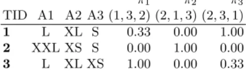
Given that the loss function that we aim to minimize is known beforehand, it makes sense to use it to measure the similarity between rankings. Therefore, we use Kendall’sτ. In this case, we think thatθsup= 0 would be a reasonable value, given that it separates the negative from the positive contributions. Table 1 shows an example of a label ranking dataset represented following this approach. To present a more clear interpretation, the example given in Table 1, the instance
({A1 =L, A2 =XL, A3 =S}) (T ID= 1) contributes 1 to the support count of the ruleitem:
Table 1.An example of a label ranking dataset to be processed by the APRIORI-LR algorithm. π1 π2 π3 TID A1 A2 A3 (1,3,2) (2,1,3) (2,3,1) 1 L XL S 0.33 0.00 1.00 2 XXL XS S 0.00 1.00 0.00 3 L XL XS 1.00 0.00 0.33
The same instance will also give a small contribution of 0.33 to the support count of the ruleitem
h{A1 =L, A2 =XL, A3 =S}, π1i
given their similarity. On the other hand, no contribution is given to the count used for the support of ruleitem
h{A1 =L, A2 =XL, A3 =S}, π2i
which makes sense as they are clearly different.
3
Discretization
Several Data Mining (DM) algorithms can improve their performance by us-ing discretized versions of continuous-valued attributes [9]. Given that a large number of algorithms, like the Naive Bayes classifier, cannot work without dis-cretized data [13] and the majority of real datasets have continuous variables, a good discretization method can be very relevant for the accuracy of the models. Discretization methods deal with continuous variables by partitioning them into intervals or ranges. Then, each of these intervals can be interpreted as a nominal value by DM algorithms.
The main issue in discretization is the choice of the intervals because a con-tinuous variable can be discretized in an infinite number of ways. An ideal dis-cretization method finds a reasonable number6 of cut points that split the data into meaningful intervals. For classification datasets, a meaningful interval should be coherent with the class distribution along the variable.
Discretization approaches can be divided into two groups:
Supervised vs Unsupervised When dealing with classification datasets the dis-cretization methods can use the values of the target variable or not. These are re-ferred to assupervisedandunsupervisedrespectively. Theunsupervised methods ignore the classes of the objects and divide the interval into a user-defined num-ber of bins. Supervised methods take into account the distribution of the class labels in the discretization process. Previous research states that the supervised methods tend to produce better discretizations than unsupervised methods [8].
6
An extreme discretization approach would create one nominal value for each contin-uous value but this is naturally not a reasonable approach.
Top-down vs Bottom-up Discretization methods with a Top-down or Bottom-up approach start by sorting the dataset with respect to the variable which will be discretized. In the Top-down approach, the method starts with an interval containing all points. Then, it recursively splits the intervals into sub-intervals, until a stopping criteria is reached.
In the Bottom-up approach, the method starts with the maximum number of intervals (i.e., one for each value) and then iteratively merges them recursively until a stopping criteria is satisfied.
3.1 Entropy based methods
Several methods, such as [6, 10], perform discretization by optimizing entropy. In classification, class entropy is a measure of uncertainty in a finite interval of classes and it can be used in the search of candidate partitions. A good partition is such that it minimizes the overall entropy in its subsets. Likewise, in discretization, a good partition of the continuous variable minimizes the class entropy in the subsets of examples it creates. In [10] it was shown that optimal cut points must be between instances of distinct classes. In practical terms, for all possible partitions the class information entropy is calculated and compared with the entropy without partitions. This can be done recursively until some stopping criterion is satisfied. The stopping criteria can be defined by a user or by a heuristic method like MDLP.
4
Discretization for Label Ranking
A supervised discretization method for LR should take into account the prop-erties of rankings as target variables. In this work, we propose an adaptation of the Shannon entropy for rankings. This entropy will be used in conjuction with MDLP as stopping criterion, the same way it is used for classification. First we describe our adaptation of the entropy for rankings and then we show how to integrate it with MDLP.
The entropy of classes presented in [10], which derives from the Shannon entropy, is defined as:
Ent(S) =−
k
X
i=1
P(Ci, S)log(P(Ci, S)) (2)
whereP(Ci, S) stands for the proportion of examples with classCi in a subset S andkis the total number of classes inS.
P(Ci, S) =#Ci N N is the number of instances in the subsetS.
As shown in equation 2 the Shannon entropy of a set of classes depends on the relative proportion of each class.
4.1 Entropy of rankings
In this section, we explain how to adapt the entropy of classes used in [10] for LR. We start by motivating our approach with a discussion of the use in LR of the concept of entropy from classification. We then show in detail our heuristic adaptation of entropy for rankings.
To better motivate and explain our approach, we introduce a very simple synthetic dataset,Dex, presented in Table 2. In this test dataset we have eight distinct rankings in the target column π. Even though they are all distinct, the first five are very similar (the label ranks are mostly ascending), but very different from the last three (mostly descending ranks). Without any further considerations, it is natural to assume that an optimal split point forDexshould lie between values 0.5 and 0.6 (instances 5 and 6).
Table 2.Example datasetDex: Small artificial dataset with some noise in the rankings
TID Att π λ 1 0.1 (1,2,4,3,5) a 2 0.2 (1,2,3,4,5) b 3 0.3 (2,1,3,4,5) c 4 0.4 (1,3,2,4,5) d 5 0.5 (1,2,3,5,4) e 6 0.6 (5,4,3,1,2) f 7 0.7 (4,5,3,2,1) g 8 0.8 (5,3,4,2,1) h
In the RAC approach, the rankings are transformed into eight distinct classes as shown in columnλ. As the table shows, the natural split point identified earlier is completely undetectable in columnλ.
As shown in equation 2, the entropy of a set of classes depends on the relative proportion of a class. If we measure the ranking proportion the same way, we get:
P(πi, S) = 1/8,∀πi∈Dex
We adapt this concept using the same ranking distance-based approach used to adapt the support for LRAR in APRIORI-LR [7] (equation 3). In fact, a similar line of reasoning as the one in Section 2.1 can be followed here. The uncertainty associated with a certain ranking decreases in the presence of similar – although not equal – rankings. Furthermore, this decrease is proportional to that distance. Pπ(πi, S) = PN j=1s(πi, πj) PK i=1 PN j=1s(πi, πj) (3)
WhereK is the number of distinct rankings inS.
As in [7], we use Kendallτ and the negative correlations are ignored (sec-tion 2.1). Note that a parallel can also be established with the frequentist view
used in entropy. Since Kendall τ is computed from the proportion of concor-dant pairs of labels, this can be seen as the proportion of concorconcor-dant pairwise comparisons.
However, this approach alone is not enough to give a fair measure for the entropy of rankings. The entropy of the set of classes {λ1, λ2} is the same as {λ1, λ3} or {λ2, λ3}. This happens because, λ1 is as different from λ2 as λ2 is
from λ3. However, in LR, distinct rankings can range fromcompletely different
tovery similar. Considering these two sets:
1){(1,2,3,4,5),(1,2,3,5,4)}
2){(1,2,3,4,5),(5,4,3,2,1)}
and since the ranking proportions will be the same in 1) and 2), the entropy will be the same. Also, from a pairwise-comparison point of view, the two similar rankings in set 1) match 14 pairs from a total of 15, while the rankings in 2) do not match any.
Considering that entropy is a measure of disorder, we believe that it makes sense to expect lower entropy for sets with similar rankings and bigger entropy for sets with completely different rankings.
For this reason we propose to add an extra parameter in the formula of entropy for rankings (equation 4) to force lower values on sets of similar rankings. This means we have to adapt Shannon entropy for a set of rankings to be more sensitive to the similarity of the rankings present in the set.
EntLR(S) = K
X
i=1
P(πi, S)log(P(πi, S))log(Q(πi, S)) (4)
where Q(πi, S) is the average similarity of the rankingπi with the rankings in the subsetS defined as:
Q(πi, S) =
PN
j=1s(πi, πj)
N (5)
For the same reason we find noise in independent variables, it is expected to observe the same phenomenon in ranking data. As the number of labels in-creases, we expect to observe it with more frequency, since the number of possible combinations for k labels grows to k!. As an example, instances 6, 7 and 8 in Dexcan correspond to observations of the same “real” ranking, say (5,4,3,2,1), but with some noise.
This measure of entropy for rankings we propose here will make the dis-cretization method more robust to noise present in the rankings. In order to support this statement we provide an analysis of the behavior of the method with induced and controlled noise.
The results presented do not include an analysis on partial orders. Given that, Kendallτ is a measure of the proportion of the concordant pairs of labels, this entropy measure can still work with partial orders, as long as there is at least one pairwise per instance.
4.2 MDLP for LR
MDLP [10] is a well known method used to discretize continuous attributes for classification learning. The method tries to maximize the information gain and considers all the classes of the data as completely distinct classes. For this reason, we believe that the latter, as is, is not suitable for datasets which have rankings instead of classes in the target.
MDLP measures the information gain of a given split point by comparing the values of entropy. For each split point considered, the entropy of the initial interval is compared with the weighted sum of the entropy of the two resulting intervals. Given an intervalS:
GainLR(A, T;S) =EntLR(S)−
|S1|
N EntLR(S1)−
|S2|
N EntLR(S2) Where |S1| and |S2| is the number of instances in the left side (S1) and the
number of instances in the right side (S2) of the cut pointT, respectively, in the
attributeA.
After the adaptation of entropy for sets of rankings proposed in Section 4.1, Minimum Description Length Principle for Ranking data (MDLP-R) comes in a natural way. We only need to replace the entropy for rankings in the MDLP definition presented in [10], which we transcribe below:
MDLPC Criterion The partition induced by a cut point T for a set S of N examples is accepted iff
GainLR(A, T;S)>
log2(N−1)
N +
∆LR(A, T;S) N and it is rejected otherwise.
Where∆LR(A, T;S) is equal to:
log2 3K−2−[KEntLR(S)−K1EntLR(S1)−K2EntLR(S2)]
5
Experimental Results
Since what we are proposing is essentially a pre-processing method, the quality of its discretization is hard to measure in a direct way. For this reason, the experimental setup is divided in two parts. In the first part we present the results obtained from controlled artificial datasets that should give an indication whether the method is performing as expected. The second part shows results of the APRIORI-LR algorithm [7] run on datasets from the KEBI Data Repository at Philipps University of Marburg [3].
Table 3 compares the intervals discretized by the MDLP-R and MDLP in dataset Dex. As expected, since there are eight distinct rankings, the RAC ap-proach with MDLP for classification will see eight distinct classes and break the dataset into eight intervals. MDLP-R, however, can identify the similarities of rankings, and only breaks the dataset into two intervals.
Table 4 gives a description of the benchmark datasets from KEBI Data Repository at Philipps University of Marburg [3].
Table 3.Discretization results using the MDLP and MDLP-R methods Partitions TID Att π λMDLP-R MDLP 1 0.1 (1,2,4,3,5) a 1 1 2 0.2 (1,2,3,4,5) b 1 2 3 0.3 (2,1,3,4,5) c 1 3 4 0.4 (1,3,2,4,5) d 1 4 5 0.5 (1,2,3,5,4) e 1 5 6 0.6 (5,4,3,1,2) f 2 6 7 0.7 (4,5,3,2,1) g 2 7 8 0.8 (5,3,4,2,1) h 2 8
Table 4.Summary of the datasets
Datasets type #examples #labels #attributes
autorship A 841 4 70 bodyfat B 252 7 7 calhousing B 20640 4 4 cpu-small B 8192 5 6 elevators B 16599 9 9 fried B 40769 5 9 glass A 214 6 9 housing B 506 6 6 iris A 150 3 4 segment A 2310 7 18 stock B 950 5 5 vehicle A 846 4 18 vowel A 528 11 10 wine A 178 3 13 wisconsin B 194 16 16
5.1 Results on artificial datasets
Results obtained with artificial datasets can give more insight about how the discretization method performs. The synthetic datasets presented in this sec-tion are variasec-tions of a simple one which has only two initial rankings π1 =
(1,2,3,4,5,6,7,8,9,10) andπ2= (10,9,8,7,6,5,4,3,2,1). To make it as simple
as possible, it has only one independent variable which varies from 1 to 100. The first 60 instances are variations of π1 and the remaining are variations ofπ2.
In order to test the advantages of our method in comparison with the RAC approach, we intentionally introduced noise in the target rankings, by performing several swaps. Each swap is an inversion of two consecutive ranks in every ranking of the data. For each ranking the choice of the pairs to invert is random. Swaps will be done repeatedly, to obtain different levels of noise.
We performed an experiment which varies the number of swaps from 0 to 100. The greater the number of consecutive swaps, the more chaotic the dataset will be, and hence more difficult to discretize.
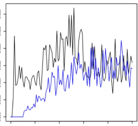
0 20 40 60 80 100 0.2 0.4 0.6 0.8 1.0 #Swaps K endall tau
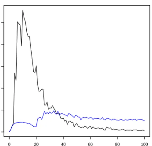
Fig. 1.Accuracy of the APRIORI-LR (expressed in terms of Kendallτ) as a function of the number of swaps, for MDLP (black) and MDLP-LR (blue).
0 20 40 60 80 100 0.000 0.005 0.010 0.015 0.020 0.025 0.030 #Swaps K endall tau
Fig. 2. Standard deviation of the ac-curacy of APRIORI-LR (in terms of Kendall τ) after discretization with MDLP-R (blue) and MDLP (black).
Figure 1 compares the accuracy of APRIORI-LR with two different dis-cretization methods, MDLP and MDLP-R. The graph, clearly indicates that the discretization with MDLP-R (blue line) leads to better results for APRIORI-LR, than with MDLP after a RAC transformation . While for the first cases the difference is not so evident, as the noise increases, MDLP-R gives a greater contribution.
However, if we analyze Figure 2 there is extra information in favor of MDLP-R. The standard deviation of the 10 runs of the 10-fold cross-validation is zero in the presence of small amounts of noise (until approximately 10 swaps). This means that, in a scenario with reasonable noise in rankings, if one decides to use MDLP-R there are more chances to get the best result than with MDLP.
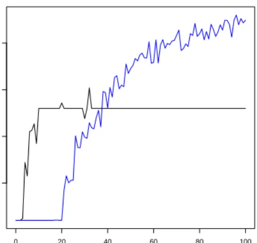
One great advantage of our method in this experiment can be seen in Fig-ure 3. In particular, for any number of swaps until 20, our method only makes one partition which means that the split point choice is also invariant to a rea-sonable amount of noise. This will result in a small number of rules generated by APRIORI-LR as supported by the graph in Figure 4. In other words, MDLP-R makes APRIORI-LR much more efficient because it only needs to create approx-imately 1/10 of the rules to obtain the same accuracy.
In Figure 5 we can see the percentage of instances from the test set that were not ranked with the default rule. Since the minimum confidence was set to 50%
0 20 40 60 80 100 10 20 30 40 #Swaps #P ar titions
Fig. 3.Comparison of the average number of partitions generated by MDLP-R (blue) and MDLP (black)
from this graph we can conclude that ARIORI-LR with MDLP is decreasing the number of rules with confidence equal or higher than 50%. Thus, MDLP-R creates more meaningful intervals which lead to higher confidence LRAR.
Additionally, in Figure 3 it is clear that, from a certain point, MDLP is no longer able to make the distinction of the target attributes and so the average number of partitions stays constant. On the other hand, the number of partitions by MDLP-R increases as the noise increases too, which is an indicator that our method is able to perform discretization even in complex situations.
5.2 Results on benchmark datasets
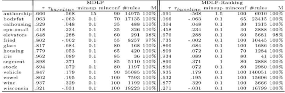
The evaluation measure is Kendall’s τ and the performance of the method was estimated using ten-fold cross-validation. For the generation of Label Ranking Association Rules (LR-AR) we used CAREN [2].
The similarity parameters used for the experiments are the same as used in [7]. The minimum support (minsup) was set to 0.1%. However, in some datasets, namely those with a larger number of attributes, frequent rule generation can be a very time consuming task. In this case, minsup was set to a larger value, 1% or higher.
When the algorithm cannot find at least one LRAR to rank a new instance, a default ranking is used. Since the usage of the default rule is only used as a last resourt, the minimum confidence (minconf) was adjusted with the same method used in [7] for parameter tunning. The latter aims to increase the percentage of test examples ranked without recourse to the default rule. This percentage is shown in columnM in Table 5.
Table 5 shows that both methods obtain similar results in benchmark datasets. As we observed in the results from artificial datasets, the number of rules
0 20 40 60 80 100 0 200 400 600 800 1000 #Swaps #Rules
Fig. 4.Comparison of the number of rules generated by APRIORI-LR after discretiza-tion with MDLP-R (blue) and MDLP (black)
0 20 40 60 80 100 0.2 0.4 0.6 0.8 1.0 #Swaps % of predictions
Fig. 5. Comparison of the percentage of instances from the test set that were not ranked with the default rule. MDLP-R (blue) MDLP (black)
generated after a MDLP-R discretization is higher than with MDLP in more noisy/complex datasets. This is due to a higher number of partitions. The same phenomenon is also clear in Table 5 where the number of rules is generally higher with a MDLP-R discretization.
A baseline method uses the default LRAR, which is a rule with the average ranking, and the accuracy is presented in columnτbaseline as show in Table 5
Table 5.Results obtained with MDLP discretization and withMDLP-Rdiscretization on bechmark datasets
MDLP MDLP-Ranking
τ τbaselineminsup minconf #rules M τ τbaselineminsup minconf #rules M authorship .666 .568 15 90 14975 100% .691 -568 1.5 100 6010 100% bodyfat .063 -.063 0.1 70 17135 100% .066 -.063 0.1 65 23415 100% calhousing .329 .048 0.1 35 488 100% .304 .048 0.1 30 1315 100% cpu-small .418 .234 0.1 35 326 100% .458 .234 0.1 40 3888 100% elevators .648 .288 0.1 60 291 98% .670 .288 0.1 60 5681 98% fried .802 -.002 0.1 55 8257 97% .735 -.002 0.1 100 10445 100% glass .817 .684 0.1 80 168 100% .860 .684 0.1 100 1686 100% housing .779 .053 0.1 65 420 100% .809 .072 0.1 70 1284 100% iris .962 .089 0.1 85 36 100% .934 .089 0.1 80 41 100% segment .898 .371 1 85 5110 100% .890 .371 1 80 2888 100% stock .894 .072 0.1 80 1197 100% .890 .072 0.1 80 2980 100% vehicle .847 .179 0.1 90 35085 100% .835 .179 0.1 100 140051 100% vowel .802 .195 0.1 100 7593 100% .632 .195 0.1 100 15606 100% wine .937 .329 0.1 100 1192 100% .877 .329 0.1 100 3666 100% wisconsin .321 -.031 0.1 100 18223 100% .271 -.031 0.1 100 16799 100%
6
Conclusions
In his paper we present a simple adaptation of the supervised discretization method, MDLP, for LR. This work was motivated by the lack of supervised discretization methods to deal with rankings in the target variable. The results clearly show that this is a viable LR method.
Our method clearly outperforms MDLP in the experiments with artificial data. In this work we empirically show that, in simple scenarios, MDLP-R deals with noisy ranking data accordingly to expected. Hence the latter is more reli-able, in this kind of situation, than MDLP.
In Section 5.1 there are two sides of the new MDLP-R. In the presence of very simple LR problems (#swaps≤20), it has less partitions and APRIORI-LR generates fewer rules than with MDLP. On the other hand, in more complex situations (#swaps >20) it has more partitions than MDLP and, consequently, APRIORI-LR creates more rules. The latter, in our opinion, cannot be seen as a disadvantage. The fact that there are more partitions being made means that the method is still able to identify similar groups of rankings even in very complex cases.
We believe that the measure of entropy for rankings proposed here, despite its heuristic nature, makes sense and its useful in the LR field. This new measure and MDLP-R bring new possibilities for processing ranking data and can motivate the creation of new methods for LR learning that cannot deal with continuous data. Furthermore, even though it was developed in the context of the LR task, it can be also applied to other fields such as regression since it is based on a distance measure such as Kendallτ.
This work uncovered several possibilities that could be better studied in order to improve the discretization in the LR field. They include: the choice of parameters in the stopping criterion; the usage of other entropy measures for rankings.
We also believe that it is essential to test the methods on real LR prob-lems like metalearnig or predicting the rankings of financial analysts [1]. The KEBI datasets are adapted from UCI classification problems. In terms of real
world applications, these can be adapted to rank analysts, based on their past performance and also preferences of radios, based on user’s preferences.
Acknowledgments
This work was partially supported by Project Best-Case, which is co-financed by the North Portugal Regional Operational Programme (ON.2 - O Novo Norte), under the National Strategic Reference Framework (NSRF), through the Euro-pean Regional Development Fund (ERDF).
We thank the anonymous referees for useful comments.
References
1. A. Aiguzhinov, C. Soares, and A. P. Serra. A similarity-based adaptation of naive bayes for label ranking: Application to the metalearning problem of algorithm recommendation. InDiscovery Science, pages 16–26, 2010.
2. P. J. Azevedo and A. M. Jorge. Ensembles of jittered association rule classifiers. Data Min. Knowl. Discov., 21(1):91–129, 2010.
3. W. Cheng, J. H¨uhn, and E. H¨ullermeier. Decision tree and instance-based learning for label ranking. In ICML ’09: Proceedings of the 26th Annual International Conference on Machine Learning, pages 161–168, New York, NY, USA, 2009. ACM. 4. W. Cheng and E. H¨ullermeier. Label ranking with abstention: Predicting par-tial orders by thresholding probability distributions (extended abstract). CoRR, abs/1112.0508, 2011.
5. W. Cheng, E. H¨ullermeier, W. Waegeman, and V. Welker. Label ranking with partial abstention based on thresholded probabilistic models. InAdvances in Neural Information Processing Systems 25, pages 2510–2518, 2012.
6. D. K. Y. Chiu, B. Cheung, and A. K. C. Wong. Information synthesis based on hierarchical maximum entropy discretization. J. Exp. Theor. Artif. Intell., 2(2):117–129, 1990.
7. C. R. de S´a, C. Soares, A. M. Jorge, P. J. Azevedo, and J. P. da Costa. Mining association rules for label ranking. InPAKDD (2), pages 432–443, 2011.
8. J. Dougherty, R. Kohavi, and M. Sahami. Supervised and unsupervised discretiza-tion of continuous features. InMachine Learning - International Workshop Then Conference -, pages 194–202, 1995.
9. T. Elomaa and J. Rousu. Efficient multisplitting revisited: Optima-preserving elimination of partition candidates. Data Min. Knowl. Discov., 8(2):97–126, 2004. 10. U. M. Fayyad and K. B. Irani. Multi-interval discretization of continuous-valued
attributes for classification learning. InIJCAI, pages 1022–1029, 1993.
11. M. Gurrieri, X. Siebert, P. Fortemps, S. Greco, and R. Slowinski. Label ranking: A new rule-based label ranking method. InIPMU (1), pages 613–623, 2012. 12. M. Kendall and J. Gibbons. Rank correlation methods. Griffin London, 1970. 13. S. Kotsiantis and D. Kanellopoulos. Discretization techniques: A recent
sur-vey. GESTS International Transactions on Computer Science and Engineering, 32(1):47–58, 2006.
14. B. Liu, W. Hsu, and Y. Ma. Integrating classification and association rule mining. Knowledge Discovery and Data Mining, pages 80–86, 1998.
15. G. Ribeiro, W. Duivesteijn, C. Soares, and A. J. Knobbe. Multilayer perceptron for label ranking. InICANN (2), pages 25–32, 2012.
16. C. Spearman. The proof and measurement of association between two things. American Journal of Psychology, 15:72–101, 1904.