Globalization and inequality
This chapter examines the relationship between the rapid pace of trade and financial globalization and the rise in income inequality observed in most countries over the past two decades. The analysis finds that technological progress has had a greater impact than globalization on inequality within countries. The limited overall impact of globalization reflects two offsetting tendencies: whereas trade globalization is associated with a reduction in inequality, finan-cial globalization—and foreign direct investment in particular—is associated with an increase in inequal-ity. It should be emphasized that these findings are subject to a number of caveats related to data limita-tions, and it is particularly difficult to disentangle the effects of technology and financial globalization since they both work through processes that raise the demand for skilled workers. The chapter concludes that policies aimed at reducing barriers to trade and broadening access to education and credit can allow the benefits of globalization to be shared more equally.
T
he integration of the world economythrough the progressive globalization of trade and finance has reached unprece-dented levels, surpassing the pre–World War I peak. This new wave of globalization is having far-reaching implications for the eco-nomic well-being of citizens in all regions and among all income groups, and is the subject of active public debate. Previous issues of the World
Economic Outlook have analyzed the impact of
glo-balization on business cycle spillovers and labor markets (April 2007), on inflation (April 2006), and on external imbalances (April 2005). This chapter makes a further contribution to the study of globalization by examining the
impli-cations for inequality and the distribution of income within countries, with a focus on emerg-ing market and developemerg-ing countries (often referred to as developing economies in the remainder of the chapter).
The debate on the distributional effects of globalization is often polarized between two points of view. One school of thought argues that globalization leads to a rising tide of income, which raises all boats. Hence, even low-income groups come out as winners from globalization in absolute terms. This optimistic view has parallels with the Kuznets hypothesis from the development literature, which pro-posed that even though inequality might rise in the initial phases of industrial development, it eventually declined as the country’s
transi-tion to industrializatransi-tion was completed. The
opposing school argues that although globaliza-tion may improve overall incomes, the benefits are not shared equally among the citizens of a country, with clear losers in relative and
pos-sibly even absolute terms.2 Moreover, widening
income disparities may not only raise welfare and social concerns, but may also limit the driv-ers of growth because the opportunities created by the process of globalization may not be fully
exploited. The sustainability of globalization
will also depend on maintaining broad support across the population, which could be adversely affected by rising inequality.
Against this background, this chapter addresses the broad question of how globaliza-tion affects the distribuglobaliza-tion of income within countries and the incomes of the poorest seg-ment of the population in particular. The main
See Kuznets (955) for the original formulation of this hypothesis.
2See The Economist (2000) and Forsyth (2000) for repre-sentative views.
See Birdsall (2007) and World Bank (2006). Note: The main authors of this chapter are Subir
Lall, Florence Jaumotte, Chris Papageorgiou, and Petia Topalova, with support from Stephanie Denis and Patrick Hettinger. Nancy Birdsall and Gordon Hanson provided consultancy support.
4
objectives are to () analyze the shifting pat-terns of globalization and income distribution over the past two decades, (2) identify the main channels through which increased trade and financial globalization affect the distribution of income within a country, and () offer policy suggestions in light of the evidence that would help countries take full advantage of the oppor-tunities from globalization while also ensuring that the benefits from globalization are shared appropriately across the population.
This chapter aims to extend the considerable literature on globalization and inequality along
several dimensions. Unlike previous studies,
which focus largely on trade globalization, this chapter also analyzes various channels of finan-cial globalization to offer a more comprehensive view on the overall impact of globalization. Moreover, the chapter aims to explain changes in inequality over time across a broad range of countries, rather than explain average levels of inequality across a cross section of countries at a common point in time. The analysis also uses a new high-quality data set recently developed by the World Bank, applying a more consistent methodology than do most other studies that rely on multiple data sources of uneven qual-ity. However, data issues remain a concern in any cross-country analysis of inequality, and the results of the estimations in all such analyses must be interpreted with some caution.
To anticipate the main conclusions, the avail-able evidence does suggest that income inequal-ity has risen across most countries and regions over the past two decades, although the data are subject to substantial limitations. Neverthe-less, at the same time, average real incomes of the poorest segments of the population have increased across all regions and income groups. The analysis finds that increasing trade and financial globalization have had separately iden-tifiable and opposite effects on income distribu-tion. Trade liberalization and export growth
See Goldberg and Pavcnik (2007) for a survey of theoretical and empirical research on the distributional
are found to be associated with lower income inequality, whereas increased financial openness is associated with higher inequality. However, their combined contribution to rising inequality has been much lower than that of technological change, especially in developing countries. The spread of technology is, of course, itself related to increased globalization, but technological progress is nevertheless seen to have a separately identifiable effect on inequality.5 The
disequal-izing impact of financial openness—mainly felt through foreign direct investment (FDI)—and technological progress appear to be working through similar channels by increasing the premium on higher skills, rather than limiting opportunities for economic advancement. Con-sistent with this, increased access to education is associated with more equal income distributions on average.
The next section reviews the evidence on both globalization and inequality over the past two decades, and how they have evolved across regions and income groups. The following sec-tion discusses the channels through which trade and financial globalization may be expected to influence inequality within countries and analyzes the empirical evidence to identify the main factors explaining changes in inequality. The concluding section offers some policy sug-gestions. Box . discusses in more detail the analytical and measurement issues arising from different methodologies used to collect and summarize inequality data across countries and regions. Box .2 looks in more detail at what might be learned from more in-depth analyses of individual country experiences and discusses how the conclusions of such studies do not easily lend themselves to generalization across countries.6
5Although much of the existing economic literature on globalization treats technological change as an exogenous variable, technological progress can also be viewed as potentially an additional channel through which global-ization operates.
6See also Fishlow and Parker (999) for a detailed analysis of the link between globalization and inequality
how has Globalization evolved?
World trade has grown five times in real terms since 980, and its share of world GDP has risen from 6 percent to 55 percent over
this period (Figure .).7 Trade integration
accelerated in the 990s, as former Eastern bloc countries integrated into the global trading system and as developing Asia—one of the most closed regions to trade in 980—progressively
dismantled barriers to trade.However, it is
noteworthy that all groups of emerging market and developing countries, when aggregated by income group or by region, have been catching up with or surpassing high-income countries in their trade openness, reflecting the wide-spread convergence of low- and middle-income countries’ trade systems toward the traditionally more open trading regimes in place in advanced
economies.8
Financial globalization has also proceeded
at a very rapid pace over the past two decades.9
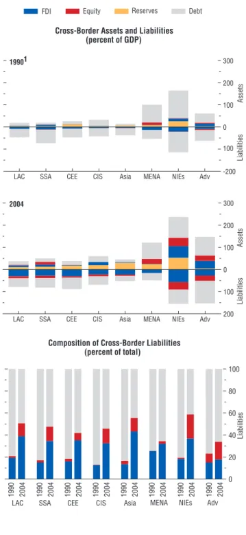
Total cross-border financial assets have more than doubled, from 58 percent of global GDP in 990 to percent in 200. The advanced economies continue to be the most financially integrated, but other regions of the world have progressively increased their cross-border asset and liability positions (Figure .2). However, de jure measures of capital account open-ness present a mixed picture, with the newly industrialized Asian economies (NIEs) and developing economies showing little evidence of convergence to the more open capital account regimes in advanced economies,
7Oil exports and imports are excluded from the trade measures but not from overall GDP. The charts in the top panel of Figure . use GDP-weighted averages, but the trends over time are similar when using simple averages.
8Country compositions of the regional and income groups are documented in Appendix ..
9For a comprehensive discussion of financial globaliza-tion and its implicaglobaliza-tions, see IMF (2007).
1980 85 90 95 2000 05 0 10 20 30 40 50 60 70 (GDP-weighted average)
“De Facto” Trade Openness (ratio of imports and exports to GDP)
1980 85 90 95 2000 05 40 50 60 70 80 90 100 110 120
Source: IMF staff calculations.
Maximum is the highest value in 2006 (Singapore). Median across countries for each year.
Data series begin in 1994 for central and eastern Europe and the Commonwealth of Independent States.
Tariff rate calculated as an average of the effective tariff rate (ratio of tariff revenue to import value) and of the average unweighted tariff rates.
1 2 3 4 1980 85 90 95 2000 05 0 20 40 60 80 100 120 140 160
180 By Region By Income Level
Low Lower middle Upper middle High 0 50 100 150 200 250 300 LA C CIS SSA MEN A
Asia CEE NIEs Adv LAC CIS SSA
MEN A Asia CEE NIEs Adv 0 5 10 15 20 25 30 35 40 45 Ratio to Median 1980 1990 2006 3 2 Ratio to Maximum1 1980 1990 2006 3 1980 85 90 95 2000 0540 50 60 70 80 90 100 110 120
By Region By Income Level “De Jure” Trade Openness
(100 minus tariff rate)
High
Low Upper middle
Lower middle
4
Trade globalization accelerated in the 1990s as countries of the former Eastern bloc integrated into the global trading system and developing Asia progressively dismantled barriers to trade.
Newly industrialized Asian economies (NIEs) Developing Asia (Asia) Commonwealth of Independent States (CIS)
Advanced economies (Adv) Latin America and the Caribbean (LAC) Middle East and north Africa (MENA) Central and eastern Europe (CEE) Sub-Saharan Africa (SSA)
which have continued to liberalize further. Of note, the share of FDI in total liabilities has risen across all emerging markets—from 7 percent of their total liabilities in 990 to 8 percent in 200—and far exceeds the share of portfolio equity liabilities, which rose from 2 percent to percent of total liabilities over the same period. Reduced government bor-rowing needs have also contributed to chang-ing liability structures, with the share of debt in total liabilities falling across all emerging market and developing country regions. Not surprisingly, the share of international reserves in cross-border assets has also risen, reflect-ing the accumulation of reserves among many emerging market and developing countries in recent years.
has income distribution Within Countries become less equal?
Cross-country comparisons of inequality are generally plagued by problems of poor reliability, lack of coverage, and inconsistent
methodology. Some of these issues are
dis-cussed in more detail in Box .. This chapter relies on inequality data from the latest World Bank Povcal database constructed by Chen and Ravallion (200, 2007) for a large number of developing countries. This database uses a more rigorous approach to filtering the individual income and consumption data for differences in quality than other commonly used databases, which rely on more mechanical approaches
0Both de facto and de jure measures have advantages and disadvantages, and are typically seen as complements rather than substitutes in empirical studies. See Kose and others (2006) for a discussion.
Taking an alternative approach, Milanovic (2005b, 2006) and World Bank (2007) review patterns of global income inequality, that is, income inequality across the world’s citizens, and their relation to globalization. Such studies typically conclude that global income inequal-ity has declined with the increase in per capita incomes in developing countries that globalization has fostered. Policy implications within countries of such analysis are less clear. A related branch of research on cross-country income inequality focuses on the impact of globalization
199 0 2004 199 0 2004 199 0 2004 199 0 2004 199 0 2004 199 0 2004 199 0 2004 199 0 2004 0 20 40 60 80 100 LAC SSA CEE CIS Asia MENA NIEs Adv 200
100 0 100 200 300 LAC SSA CEE CIS Asia MENA NIEs Adv -200 0 100
100 200 300
Figure 4.2. Financial Globalization
(GDP-weighted average)
The advanced economies (including the NIEs) continue to have the largest amount of cross-border financial assets and liabilities, but other regions of the world have also progressively increased their cross-border asset and liability positions.
FDI Equity Reserves Debt
Cross-Border Assets and Liabilities (percent of GDP) Assets Liabilities 19901 Assets Liabilities 2004 Liabilitie s
LAC SSA CEE CIS Asia MENA NIEs Adv Composition of Cross-Border Liabilities
data from the Luxembourg Income Study (LIS) database, which provides high-quality coverage for advanced economies, and the resulting full sample allows for more accurate within- and cross-country comparisons than are available elsewhere. Given limitations of data availability, the analysis in this chapter uses inequality data based on both income and expenditure surveys. Mixing these two concepts makes a compari-son of levels of inequality across countries and
regions potentially misleading. Given the
difficulty in comparing inequality levels across countries, this section discusses them briefly and focuses instead on changes, whereas the empirical analysis relies solely on changes in inequality to avoid the biases inherent in level estimations.
Based on observed movements in Gini coef-ficients (the most widely used summary measure of inequality), inequality has risen in all but the low-income country aggregates over the past two decades, although there are significant regional
and country differences (Figure .). While
inequality has risen in developing Asia, emerg-ing Europe, Latin America, the NIEs, and the advanced economies over the past two decades, it has declined in sub-Saharan Africa and the
2This database is available via the Internet at iresearch.worldbank.org/PovcalNet. Other databases include, for example, Deininger and Squire (998) and the World Income Inequality Database (2005), which includes an update of the Deininger-Squire database; the Luxembourg Income Study; and a large number of data series from central statistical offices and research studies.
See Deaton and Zaidi (2002) and Atkinson and Bourguignon (2000). Most advanced and Latin American economies construct inequality indices from income data, whereas most African and developing Asian countries use consumption data. World Bank (2006) illustrates how consumption-based Gini coefficients tend to show less inequality, in part because of government spending programs.
The Gini coefficient is computed as the average difference between all pairs of incomes in a country, nor-malized by the mean (see Box .). Other measures of inequality include decile and quintile ratios, the Atkinson index, and Theil’s entropy measure.
"De Facto" Financial Openness (ratio of assets and liabilities to GDP)
Figure 4.2 (concluded)
"De Jure" Financial Openness (capital account openness index)4
1980 85 90 95 2000 -2 -1 0 1 2 3 4 By Region 1980 85 90 95 2000 -2 -1 0 1 2 3 4 By Income Level High Low Upper middle Lower middle
Sources: Chinn and Ito (2006); Lane and Milesi-Ferretti (2006); and IMF staff calculations.
Data series begin in 1995 for central and eastern Europe and the Commonwealth of Independent States.
Maximum is the highest value in 2004 (Ireland). Median across countries for each year.
Index measuring a country's degree of capital account openness based on principal components extracted from disaggregated capital and current account restriction measures. 1 2 3 4 0 50 100 150 200 250 300
Asia LAC CEE CIS SSA
MENA NIEs Adv Asia LAC CEE CIS SSA MENA NIEs Adv 0 5 10 15 20 25 Ratio to Median 1980 1990 2006 1 3 Ratio to Maximum2 1980 1990 2006 1
Newly industrialized Asian economies (NIEs) Developing Asia (Asia) Commonwealth of Independent States (CIS)
Advanced economies (Adv) Latin America and the Caribbean (LAC) Middle East and north Africa (MENA) Central and eastern Europe (CEE) Sub-Saharan Africa (SSA)
Commonwealth of Independent States (CIS). This pattern remains broadly unchanged using population-weighted averages, except for emerg-ing market countries in Latin America, as a result of the recent declines in inequality in Brazil and Mexico. Among the largest advanced economies, inequality appears to have declined only in France, whereas among the major emerging market countries, trends are more diverse, with sharply rising inequality in China, little change in India, and falling inequality
in Brazil, Mexico, and Russia.6 These overall
measures of inequality do not, however, capture all country-specific characteristics of inequal-ity within countries. As Box .2 illustrates, a different method of aggregation of rural and urban inequality in China leads to a substan-tially less sharp increase in overall inequality, whereas in India there is substantial variation in the experience of individual rural and urban districts despite the relatively small changes at the national level.
A more detailed picture of inequality is revealed by examining income shares for dif-ferent country groups (Figure .). Overall, changes in income shares by quintile (succes-sive subsets with each containing 20 percent of the population) across regions and income levels mirror the evidence on inequality from Gini coefficients. However, the data show that rising Gini coefficients are explained largely by the increasing share of the richer quintiles
5Among the CIS countries, available evidence suggests that the sharp drop in inequality is partly a result of the reversal of the abrupt deterioration in income distribu-tion during the initial stages of transidistribu-tion. See World Bank (2000), which suggests that inequality was substan-tially higher in the early 990s in these countries.
6In a previous phase of (mainly trade) globalization, the East Asian economies grew rapidly during 965–89, while income distribution either improved or did not worsen. In addition to active government policies and reforms such as land reforms, public housing, invest-ments in health and rural infrastructure, and a manu-facturing export-oriented growth strategy, investment in education is cited as an important factor explaining low average inequality (see Birdsall, Ross, and Sabot, 995). However, data on inequality during this phase are highly Sources: Choi (2006); Povcal database; WIDER database; and IMF staff calculations.
Country coverage and years shown are limited to maintain constant country coverage. See Appendix 4.1.
Excludes Hong Kong SAR due to data unavailability.
Trends after 2000 are based on earnings data for full-time, year-round workers. 1 2 1980 85 90 95 2000 05 20 30 40 50 60 70
Figure 4.3. Cross-Country Trends in Inequality
(Gini coefficient)
Advanced economies Newly industrialized Asian economies
Latin America and the Caribbean Sub-Saharan Africa
Central and eastern Europe Commonwealth of Independent States Developing Asia
Middle East and north Africa
1985 90 95 2000 0520 30 40 50 60 1985 90 95 2000 05 20 30 40 50
60 Simple Average Population-Weighted Average Average of Country Gini Coefficients by Region
1985 90 95 2000 0520 30 40 50 60 1985 90 95 2000 05 20 30 40 50
60 Simple Average Population-Weighted Average Average of Country Gini Coefficients by Income Group
1980 85 90 95 2000 0520 30 40 50 60 70
Advanced Economies Emerging Market Economies Gini Coefficients in Selected Countries High income
Upper middle income Lower middle incomeLow income
France United Kingdom
Italy
Japan
Brazil South Africa Mexico
Russia China
India Germany4
Inequality has risen in developing Asia, central and eastern Europe, the NIEs, and the advanced economies, while falling in the Commonwealth of Independent States and, to a lesser extent, in sub-Saharan Africa.
2 United States3 3 1 1 4 Global Global
changes little. Looking at average income levels across quintiles, per capita incomes have risen across virtually all regions for even the poorest quintiles (Figures .5 and .6). The exception is Latin America, where there was a small overall decline, driven mainly by the adverse impact of economic and financial crises on the poor in several countries. However, incomes have since recovered from post-crisis lows. In fact, con-sistent with the evidence from the Gini coeffi-cients, the incomes of the poorest quintile have risen faster than those of other segments of the population in sub-Saharan Africa and the CIS countries, although from a very low base. Across all regions, the evidence therefore suggests that in an absolute sense the poor are no worse off (except in a few post-crisis economies), and in most cases significantly better off, during the most recent phase of globalization.
In summary, two broad facts emerge from the evidence. First, over the past two decades, income growth has been positive for all quintiles in virtually all regions and all income groups during the recent period of globalization. At the same time, however, income inequality has increased mainly in middle- and high-income countries, and less so in low-income countries. This recent experience seems to be a clear change in course from the general decline in inequality in the first half of the twentieth cen-tury, and the perception that East Asia’s rapid growth during the 960s and 970s was achieved while maintaining inequality at relatively low levels. It must be emphasized, however, that comparison of inequality data across decades is fraught with difficulty, in view of numerous caveats about data accuracy and methodological comparability.
What is the impact of Globalization
on inequality?
Against this background, it is natural to ask how much of the rise in inequality seen in middle- and high-income countries in recent
LAC SSA CEE CIS Asia NIEs MENA Adv Sources: Choi (2006); Japanese Statistics Bureau; Povcal database; WIDER database; and IMF staff calculations.
Data cover advanced economies (Adv), newly industrialized Asian economies (NIEs), developing Asia (Asia), Latin America and the Caribbean (LAC), sub-Saharan Africa (SSA), Middle East and north Africa (MENA), central and eastern Europe (CEE), and the Commonwealth of Independent States (CIS).
Includes only Korea and Taiwan Province of China. 1
Figure 4.4. Income Shares by Quintile
(Share of total income, population-weighted average)
0 10 20 30 40 50 60 70 80 90 100 By Region1 2
Increasing inequality is largely explained by the increasing income share of the richest quintile at the expense of the middle quintiles, while there has been little change in the poorest quintile.
Quintile 1 (poorest) Quintile 4 Quintile 2 Quintile 5 (richest) Quintile 3 1994 200 4 1994 2002 1996 2003 1996 2003 1992 2002 1990 2000 1990 2000 1990 2000 0 10 20 30 40 50 60 70 80 90 100 By Income Group Low income 200 0 1990 2000 1990 2000 1992 2002 1992 1990 Lower middle income 200 0 Upper middle
income High income Global
decades can be attributed to increased global-ization, and how much to other factors, such as the spread of technology and domestic con-straints on equality of opportunity. This section first discusses the channels through which the globalization of trade and finance could affect the distribution of incomes within a country, setting the stage for the empirical analysis that follows.
Channels through Which Globalization affects inequality
The principal analytical link between trade liberalization and income inequality provided by economic theory is derived from the Stolper-Samuelson theorem: it implies that in a two-country two-factor framework, increased trade openness (through tariff reduction) in a devel-oping country where low-skilled labor is abun-dant would result in an increase in the wages of low-skilled workers and a reduction in the compensation of high-skilled workers, leading to a reduction in income inequality (see Stolper and Samuelson, 9). After tariffs on imports are reduced, the price of the (importable) high-skill-intensive product declines and so does the compensation of the scarce high-skilled workers, whereas the price of the (exportable) low-skill-intensive good for which the country has relatively abundant factors increases and so does the compensation of low-skilled workers. For an advanced economy in which high-skill factors are relatively abundant, the reverse would hold, with an increase in openness leading to higher inequality.
An important extension of the basic model that weakens the dichotomy between advanced and developing economies in terms of distribu-tional effects is the inclusion of “noncompeting” traded goods, that is, goods that are not pro-duced in a country and are imported only as a result, for example, of very large differences in endowments across countries. Tariff reductions would reduce the prices of these goods—and therefore increase the effective real income of households—without affecting wages and prices
Sources: Choi (2006); Heston, Summers, and Aten (2006); Japanese Statistics Bureau; Povcal database; WIDER database; and IMF staff calculations.
Income or consumption share data are applied to real GDP per capita levels from Penn World Tables to calculate per capita income by quintile. See Appendix 4.1.
1
Figure 4.5. Per Capita Income by Quintile
(2000 international dollars, population-weighted average)
0 5000 10000 15000 20000 25000 0 2 4 6 8 10
Incomes have risen for all quintiles across all regions except for the poorest quintile in Latin America, related in part to the aftereffects of crises.
1993 2003
Latin America and the Caribbean 0 5000 10000 15000 20000 25000 0 2 4 6 8 10 Sub-Saharan Africa 0 5000 10000 15000 20000 25000 0 2 4 6 8 10
Central and Eastern Europe 0 5000 10000 15000 20000 25000 0 2 4 6 8 10 Commonwealth of Independent States 0 5000 10000 15000 20000 25000 0 2 4 6 8 10 Developing Asia 0 5000 10000 15000 20000 25000 0 2 4 6 8 10
Middle East and North Africa 0 5000 10000 15000 20000 25000 30000 35000 0 2 4 6 8 10
Newly Industrialized Asian Economies (NIEs) 0 10000 20000 30000 40000 50000 60000 0 2 4 6 8 10 Advanced Economies, excluding NIEs 2
Average annual growth in percent (right scale)
1994 2002 1996 2003 1996 2003 1992 2002 1990 2000 1990 2000 1990 2000 1 2 3 4 5 Quintile 1 2 3 4 5 Quintile 1 2 3 4 5 Quintile 1 2 3 4 5 Quintile 1 2 3 4 5 Quintile 1 2 3 4 5 Quintile 1 2 3 4 5 Quintile 1 2 3 4 5 Quintile -1 1
Sources: Heston, Summers, and Aten (2006); Japanese Statistics Bureau; Povcal database; WIDER database; and IMF staff calculations. Calculations are based on income share data except for India, Japan, Mexico, and Russia, where consumption share data are used. The income or consumption share data are applied to real GDP per capita levels from Penn World Tables to calculate per capita income by quintile. See Appendix 4.1. Based on household income share data.
1
Figure 4.6. Per Capita Income by Quintile in Selected Countries
(2000 international dollars) 0 5000 10000 15000 20000 25000 0 2 4 6 8 10
Despite overall increases in inequality in middle- and high-income countries, there is substantial variation in the experience of individual countries. 1996 2004 China 0 5000 10000 15000 20000 25000 0 2 4 6 8 10 India 0 5000 10000 15000 20000 25000 0 2 4 6 8 10 Brazil 0 5000 10000 15000 20000 25000 0 2 4 6 8 10 Mexico 0 10000 20000 30000 40000 0 2 4 6 8 10 Russia 0 10000 20000 30000 40000 0 2 4 6 8 10 Japan 0 10000 20000 30000 40000 50000 60000 0 2 4 6 8 10 France 0 10000 20000 30000 40000 50000 60000 0 2 4 6 8 10 United Kingdom 2
Average annual growth in percent (right scale)
1993 2003 1993 2003 1996 2004 1993 2002 1994 2004 1995 2001 1991 1999 1 2 3 4 5 Quintile 1 2 3 4 5 Quintile 1 2 3 4 5 Quintile 1 2 3 4 5 Quintile 1 2 3 4 5 Quintile 1 2 3 4 5 Quintile 1 2 3 4 5 Quintile 1 2 3 4 5 Quintile -1 0 10000 20000 30000 40000 50000 60000 70000 80000 0 2 4 6 8 10 United States 1991 2000 1 2 3 4 5 Quintile 1 2
Researchers on inequality employ several different measures, guided by the availability of underlying data and the focus of the research. Of these, the Gini index is a commonly used summary measure of the income distribution of a country.2 The Gini index captures the range between a perfectly egalitarian distribution in which all income is shared equally (a Gini coef-ficient of 0) and one where a single person has all the income (a coefficient of ). Gini coeffi-cients typically range from 0.20 to 0.65.
Despite the Gini index’s widespread use, numerous conceptual, methodological, and defi-nitional issues make it difficult to compare Gini indices across countries and over time. One major source of variation is that some Gini indi-ces are based on surveys of household consump-tion expenditure, whereas others are based on income surveys—a difference that can change a country’s observed Gini index on the order of 0.5 point. In general, consumption-based Gini indices tend to show lower inequality and are more commonly used in developing countries in which higher rates of self-employment in business or agriculture (where income fluctu-ates throughout the year) make measurement of incomes difficult. Consumption-based Gini indices are more common in Asia, sub-Saharan
Note: The main author of this box is Patrick Hettinger.
Measures of inequality include, in addition to the Gini index, ratios of the average income of the richest to poorest segments of the population, the Atkinson index, the Theil entropy measure, and the mean loga-rithmic deviation of income.
2The Gini index is defined as –––– ∑n
i= ∑ n j=
|
yi – yj|
,2n2m
where m is the mean income, yi and yj are the
indi-vidually observed incomes, and n is the number of observed incomes.
A general discussion of the difficulties in using the Gini index and data based on household surveys can be found in Deaton (200); Ravallion (200); and World Bank (2006).
Among other causes, lower measures of consumption-based inequality can result from consumption smooth-ing across time and greater measurement error for incomes. See, for example, Ravallion and Chen (996); and Meyer and Sullivan (2006).
Africa, and, more recently, in central and emerging Europe and the Commonwealth of Independent States, whereas income Ginis are commonly used in advanced economies and Latin America.5 Differences in definitions and survey methodologies further complicate the use of both consumption- and income-based Gini indices. Comparability of Gini indices based on consumption survey data can be limited as a result of differences in definitions of tion; variation in the number of consump-tion items that are separately distinguished in surveys; whether survey participants record their consumption or are asked to recall their con-sumption in an interview; changes in the length of the recall period during which survey partici-pants are asked to report their consumption; different methods used to impute housing, dura-bles, and home production consumption; incon-sistencies in the treatment of seasonality and the timing of surveys; underreporting or misleading reports of consumption of some items; and varia-tion in respondents within a household. Income inequality data can also vary depending on whether the income is pre- or post-tax; whether and how in-kind income, imputed rents, and home production are included; and whether all income—including remittances, other transfers, and property income—or only wage earnings are captured.6
More general concerns with both types of Gini indices are that some surveys are not nationally representative and exclude rural pop-ulations, the military, students, or populations living in areas that are expensive or dangerous to survey. In addition, survey nonresponse and underreporting of income—which occurs more often in the high-income groups in a country— can skew income distributions, thereby under-reporting inequality. Also, whether and how
5See, for example, Chen and Ravallion (200). 6For most advanced economies in this study, post-tax income is used, although the components of income vary across countries. See Luxembourg Income Study data as provided in the World Income Inequality Database.
of other traded goods.7 If this noncompeting
good is a large share of the consumption basket of poorer segments of society, a reduction in the tariff on the noncompeting good would reduce inequality in that country. More generally, in both advanced and developing economies, if tariffs are reduced for noncompeting goods that are not produced in a country but are con-sumed particularly by the poor, it would lead to lower inequality in both advanced and develop-ing economies.
The implications of the Stolper-Samuelson theorem, in particular the ameliorating effects of trade liberalization on income inequality in developing countries, have generally not been
verified in economy-wide studies.8 A particular
7See, for example, Davis and Mishra (2007) for an overview of analytical and empirical approaches to the relationship between trade, inequality, and poverty.
8See Milanovic (2005a) for a survey of recent papers linking trade globalization to inequality, which notes that
challenge has been to explain the increase in skill premium between skilled and unskilled workers observed in most developing coun-tries. This has led to various alternative analyti-cal approaches, including the introduction of () multiple countries where poor countries may also import low-skill-intensive goods from other poor countries and rich countries may similarly import high-skill-intensive goods from other rich countries; (2) a continuum of goods, implying that what is low-skill intensive in the advanced economy will be relatively high-skill intensive in a less-developed country (see Feenstra and Hanson, 996); and () intermediate imported goods used for the skill-intensive product. How-ever, these extensions have themselves presented additional challenges for empirical testing, and
most papers find either no statistically significant relation-ship or a negative relationrelation-ship between globalization and inequality.
a survey adjusts for price-level differences between urban and rural areas can significantly alter distribution data.
Finally, there are differences between indica-tors of household and individual inequality. Household inequality measures, which were much more common before 980, may show changing inequality over time merely as a result of changes in household size and composition. Adjusting inequality indicators to a per capita unit of analysis helps avoid this bias, and various methods have been adopted for making this adjustment.7
Although survey guidelines exist, they are not consistently applied over time and across coun-tries, so that different surveys and even different survey rounds can produce different results.8
7For several examples of how measures are adjusted, see World Income Inequality Database (2005).
8See Canberra Group (200); and Deaton and Zaidi (2002).
When comparing Gini indices, meticulous atten-tion to concepts, definiatten-tions, and the details of survey methodology is required to improve com-parability, and the World Bank’s Povcal database goes further than other databases in doing this.9 The database was created using primary data from nationally representative surveys with suf-ficiently comprehensive definitions of income or consumption. Attempts were made to ensure survey comparability over time within countries, although cross-country and within-country comparisons are still impaired because in many cases it was not possible to correct for differ-ences in survey methods. Finally, measures are calculated consistently and on a per capita basis. For the econometric analysis in this study, using changes over time in Gini indices from this database rather than levels can address some of the major concerns regarding comparability of indices across countries.
A complementary approach to the cross-country analysis of the impact of globalization on inequality used in this chapter is to look in detail at particular country experiences (see Goldberg and Pavcnik, 2007). The advantage of country studies is that they focus on more detailed measures of inequality (that is, wage inequality) and at a finer level of disaggregation geographically or by sector. In addition, they also use more detailed data for other variables, such as tariffs and social policies. Given that globalization may affect inequality through different channels and at different speeds in different countries, country studies can provide important insights that cannot be gained in cross-country work and in which policies and outcomes can be more closely related. The following overview of recent studies on Mexico, China, and India illustrates the usefulness as well as the limitations of country studies.2 Mexico
Mexico undertook far-reaching reforms between 985 and 99 that opened its economy to trade and capital flows. Over the same period, the earnings gap between high- and low-skilled workers began to widen, generating a substan-tial body of literature that examined whether this increasing gap was caused by the process of
Note: The main author of this box is Chris Papa-georgiou, with contributions by Gordon Hanson and Petia Topalova.
A limitation of most of these country studies is that they do not control explicitly for technological prog-ress and, in some cases, for financial globalization, both of which were found in this chapter to play a key role. Another limitation is the use of a difference-in-difference methodology that does not capture the countrywide effect of globalization on inequality. While liberalization may have an overall effect of increasing or lowering inequality, this methodology tests whether this overall effect was unequal, and whether certain industries or regions benefited more from globalization than others.
2Studies that focus on the experiences of Colombia, Argentina, Brazil, Chile, and Hong Kong SAR are summarized in Goldberg and Pavcnik (2007).
opening up. In broad terms, researchers have found that the patterns of trade liberalization may have contributed to increasing the earn-ings gap. Hanson and Harrison (999) find that trade protection was initially higher in less-skill-intensive sectors, and was reduced by more in these sectors during reform. If these tariff changes were passed through to changes in prices of goods, then the logic of the Stolper-Samuelson theorem would imply that the relative wage of skilled labor would have risen. Robertson (200) finds evidence in support of this conclu-sion, with the relative price of skill-intensive goods in Mexico rising during 987–9 and rais-ing the relative wages of white-collar labor.
Other studies with a slightly different focus find that although globalization may have contributed to widening earnings inequality in Mexico, low-skilled workers have benefited in absolute terms as a result of the policy changes. Nicita (200) shows that during the 990s, tariff changes raised disposable income for all house-holds, with richer households enjoying a 6 per-cent increase and poorer households enjoying a 2 percent increase, leading to a percent reduc-tion in the number of households in poverty. In a related work, Hanson (2007) finds that during the 990s, individuals in regions more exposed to globalization enjoyed a 0 percent gain in labor income relative to individuals in regions less exposed to globalization, resulting in a reduc-tion in poverty rates in high-exposure regions of 7 percent relative to low-exposure regions. China
The dramatic increase in trade liberalization in China has been accompanied by a large fall in poverty rates, but also an increase in income inequality, with the overall Gini coefficient ris-ing sharply from 0.28 in 98 to 0.2 in 200. The observed increase in overall inequality
In 988, urban workers at the 90th percentile had labor earnings that were .6 times those of workers at the 0th percentile. By 200, the ratio had grown to .7 times, with large fluctuations in relative earnings around the Mexican peso crisis in 99–95.
box 4.2. What do Country Studies of the impact of Globalization on inequality tell us? examples from Mexico, China, and india
is mostly attributed to growing differences between rural and urban household incomes and uneven growth in incomes among urban households (see top panel of the figure, from Lin, Zhuang, and Yarcia, forthcoming). Focus-ing on inequality between 988 and 995, Wei and Wu (2007) also find that the aggregate inequality numbers may obscure a more subtle pattern of underlying changes. These authors examine the effect of trade globalization on Chinese income inequality using new methods and two unique data sets on 9 urban and 0 rural Chinese regions. The first data set allows examination of urban-rural income inequal-ity and the second allows the examination of within-urban and within-rural inequality. The authors employ a decomposition of the Theil index that combines the urban-rural, intra-urban, and intra-rural inequalities into an overall measure of income inequality, arguing that their Theil decomposition approach more accurately captures the unequal effects of the different components of overall inequality.5
The first data set comes from the Urban
Statisti-cal Yearbook of China and Fifty Years of the Cities in New China: 1949–98, both published by China’s State
Statistics Bureau. The second data set consists of two surveys of households conducted in 988 and 995 by international economists and the Economics Institute of the Chinese Academy of Social Sciences. The study relies on data from urban areas and rural counties administered by cities—an administrative arrange-ment specific to China—but not rural counties admin-istered directly by prefectures.
5The Theil index is an alternative to the Gini coeffi-cient. One of the advantages of the Theil index is that because it is the weighted sum of inequality within subgroups, it is easier to decompose. The particular decomposition of the Theil index used in Wei and Wu (2007, pp. 25–26) was proposed by Shorrocks (980) and Mookherjee and Shorrocks (982). More specifically, overall inequality is given by I = VrλrIr +
VuλuIu + Vrλrlogλr + Vuλulogλu, where Vr and Vu are the
proportions of population living in rural and urban areas, respectively; λr and λu are the ratios of rural
and urban average incomes to the overall national average income, respectively; and Ir and Iu are
within-rural and within-urban Theil indices, respectively. The World Bank (997) estimates that 75 percent of the change in the overall inequality is explained by urban-rural inequality during the period 98–95.
China: Openness and Inequality in Urban and Rural Areas -2.5 -2.0 -1.5 -1.0 -0.5 0.0 0.5 1.0 1.5-0.6 -0.4 -0.2 0.0 0.2 0.4 0.6 0.8
Change of log urban/rural income ratio, 1988–9
3
Openness and Urban-Rural Income Inequality: Simple Correlation
Change of log exports to GDP ratio, 1988–93
-0.4 -0.3 -0.2 -0.1 0.0 0.1 0.2 0.3 0.4-0.2 -0.1 0.0 0.1 0.2 0.3
Openness and Within-Rural Inequality: Partial Correlation Change in Gini, 1988–9 5 Change in openness -0.3 -0.2 -0.1 0.0 0.1 0.2 0.3 0.4 0.5 0.6-0.06 -0.04 -0.02 0.00 0.02 0.04 0.06 0.08 Change in Gini, 1988–9 5
Openness and Within-Urban Inequality: Partial Correlation
Change in openness
Sources: Lin, Zhuang, and Yarcia (forthcoming); and Wei and Wu (2007).
Inequality is measured in terms of the Theil index and ranges from 0 to 1. 1 1985 90 95 99 2000 01 04 0.0 0.1 0.2 0.3 0.4
Decomposing National Inequality, 1985–2004
Rural Urban Between rural-urban
Illustrating the importance of the method of aggregation, the bottom three panels in the figure present correlations between trade open-ness and urban-rural inequality, within-rural inequality, and within-urban inequality. The authors’ formal econometric analysis, consistent with the correlations in the figure, reveals that trade liberalization reduces urban-rural income inequality, leads to a relatively small increase in intra-urban inequality, and decreases intra-rural inequality. More important, summing up the three components of inequality, the authors esti-mate that increased openness modestly reduces overall inequality.6
This finding contrasts with the more wide-spread perception that trade liberalization has contributed to the rise in income inequality in China. A key lesson from this exercise is that the appropriate decomposition and measurement of income inequality across different regions can modify the observed effect of openness on income inequality in China.
The Chinese experience does not necessarily imply that the effect of trade liberalization on income inequality suggested by this methodol-ogy would be the same in other countries, given the diverse mechanisms through which global-ization operates. Moreover, data limitations in many countries typically do not allow for the application of such a methodology.
India
India intensified reforms aimed at opening up its economy in the early 990s, through reduction in tariffs and nontariff barriers, low-ered barriers to foreign direct investment, and liberalization of restrictive domestic regulations. Kumar and Mishra (forthcoming) evaluate empirically the impact of the 99 trade liberal-ization in India on industry wages.7 The paper
6In related work using household survey data for 29 Chinese provinces for 988–200, Zhang and Wan (2006) find that trade liberalization increases the income share of the poor living in urban households.
7The data set combines microlevel data from the National Sample Survey Organisation with data on international trade protection for the years 980–2000.
uses variations in industry wage premiums and trade policy across industries and over time. Industry wage premiums are defined as the portion of individual wages that accrues to the worker’s industry affiliation after controlling for worker characteristics. Since different industries employ different proportions of skilled work-ers, changes in wage premiums translate into changes in the relative incomes of skilled and unskilled workers (see Pavcnik and others, 200; and Goldberg and Pavcnik, 2005). The results suggest that reductions in tariffs were associated with increased wages within an industry, likely reflecting productivity increases. In addition, the study finds evidence that trade liberalization has led to decreased wage inequality between skilled and unskilled workers. This is consistent with the larger tariff reductions in sectors with a higher proportion of unskilled workers.
Other studies focus on the effect of tariff changes on income inequality at the district level. Topalova (2007) relates post-liberalization variations in industrial composition across districts to the degree of opening to foreign trade and FDI across industries.8 Additional research applies a difference-in-difference methodology to investigate how consumption across the entire income distribution varied with the district’s exposure to a decline in protec-tion and the liberalizaprotec-tion of FDI. Results from this work suggest that trade liberalization led to an increase in inequality, especially in urban districts, where the incomes of the richest and those with higher education rose substantially faster relative to households at the bottom of the income distribution. Although the estimates for the rural sample are not statistically signifi-cant, across all measures of inequality the point estimates imply that a decline in tariffs is associ-ated with an increase in inequality. Moreover, there does not seem to be any relationship
8This study uses consumption-based data from 60 districts (those in the 5–6 largest states in India) and for two time periods, 987 and 999. For a detailed explanation of the data and estimation method used, see Topalova (2007).
none has been consistently established.9 This
has led to explanations for rising skill premiums based on the notion that technological change is inherently skill biased, attributing the observed increases in inequality (including in advanced economies) to exogenous technology shocks. Any empirical estimation of the overall effects of globalization therefore needs to account explic-itly for changes in technology in countries, in addition to standard trade-related variables.
An additional important qualification to the implications deriving from the Samuelson theorem relates to its assumption that labor and capital are mobile within a country but not internationally. If capital can travel across borders, the implications of the theorem weaken substantially. This channel would appear to be most evident for FDI, which is often directed at high-skill sectors in the host
economy.20 Moreover, what appears to be
rela-tively high-skill-intensive inward FDI for a less-9The level of aggregation of tariff data does not, for example, allow for clear identification of noncompet-ing imports in general and noncompetnoncompet-ing intermediate goods in particular. Furthermore, in a multicountry setting with more than one low-skill-abundant country, it is unclear which goods are exportable and which are importable.
20See Cragg and Epelbaum (996); and Behrman, Birdsall, and Székely (200).
developed country may appear to be relatively low-skill-intensive outward FDI for the advanced economy. An increase in FDI from advanced economies to developing economies could thus increase the relative demand for skilled labor in both countries, increasing inequality in both the advanced and the developing economy. The empirical evidence on these channels has provided mixed support for this view, with the impact of FDI seen as either negative, at least in
the short run, or inconclusive.2
In addition to foreign direct investment, there are other important channels through which capital flows across borders, including cross-border bank lending, portfolio debt, and equity flows. Within this broader context, some have argued that greater capital account liberaliza-tion may increase access to financial resources for the poor, whereas others have suggested that by increasing the likelihood of financial crises, greater financial openness may
disproportion-ately hurt the poor. 22 Some recent research has
2See Behrman, Birdsall, and Székely (200), who find negative effects in the short term in Latin America, and Milanovic (2005a), who suggests that the evidence from a wide sample of countries is inconclusive.
22See Agénor (2002) for a discussion of the channels through which financial integration may hurt the poor, and Fallon and Lucas (2002), who find that the evidence on the distributional effects of crises is not uniform.
between FDI and inequality within a district in either the rural or the urban samples.
Conclusion
This box demonstrates how country stud-ies can take advantage of more disaggregated and more detailed data to study the effects of globalization on inequality. However, no study can capture all aspects of this relation-ship, and each study focuses instead on some parameters of particular interest. In the case of Mexico, wage, rather than income, inequality was used to capture distributional disparities across regions. In the China example,
decom-position between urban and rural inequality was shown to be fundamental in the estimation of the globalization-inequality relationship. In the India study, detailed import-tariff data across industries and districts were used as the measure of trade openness. The results from these case studies reveal a more intricate picture of the globalization-inequality interrelation-ship that cannot be captured in cross-country studies. The evidence broadly suggests that the mechanisms through which globalization affects inequality are country- and time-specific, reflect-ing the great heterogeneity of countries and the nature and timing of their trade reforms.
found that the strength of institutions plays a crucial role: in the context of strong institutions, financial globalization may allow better consump-tion smoothing and lower volatility for the poor, but where institutions are weak, financial access is biased in favor of those with higher incomes and assets and the increase in finance from tap-ping global and not just domestic savings may
further exacerbate inequality.2 Thus, the
compo-sition of financial flows may matter, and the net impact may also be influenced by other factors, such as the quality of financial sector institutions.
In summary, analytical considerations suggest that any empirical analysis of the distributional consequences of globalization must take into account both trade and the various channels through which financial globalization oper-ates, and also account for the separate impact of technological change. Moreover, against the background of real-world patterns of trade and financial flows, theory does not provide clear guidance on whether globalization affects inequality in advanced and developing econo-mies differently.
an empirical investigation of
Globalization and inequality
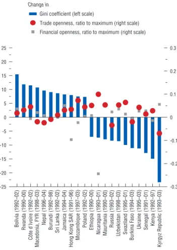
Despite common perceptions, casual obser-vation does not suggest an obvious association between changes in inequality across countries and changes in the degree to which coun-tries have globalized over the same period (Figure .7). But this is perhaps not surprising, given the multiple channels through which such a relationship would operate and the variety of other factors that are also relevant. This chapter thus looks closely at cross-country data, relating changes in inequality to a broad set of variables that may affect income distribution,
2See Prasad and others (2007) for a discussion of lower volatility from financial globalization. While Demirgüç-Kunt and Levine (2007) argue that financial development is more positive for the poorest segment of the population, primarily through its positive effect on overall growth, Claessens and Perotti (forthcoming) find that the outcome can be different as most of the benefits Sources: Lane and Milesi-Ferretti (2006); Povcal database; WIDER database; and IMF staff
calculations.
Sample includes the 11 countries with the greatest increase in Gini coefficient over the period, and the 11 countries with the greatest decrease.
Figure 4.7. Inequality Versus Globalization: Selected Countries
(Change in indicators over last available 10 years; years indicated)
-25 -20 -15 -10 -5 0 5 10 15 20 25 -0.3 -0.2 -0.1 0 0.1 0.2 0.3 Changes in inequality do not have an obvious association with changes in trade or financial openness.
Gini coefficient (left scale)
Trade openness, ratio to maximum (right scale) Financial openness, ratio to maximum (right scale)
Bolivia (1992–02) Rwanda (1990–00 ) Côte d'Ivoire (1992–02 ) Macedonia, FYR (1998–03 ) Nepal (1996–04 )
Burundi (1992–98) Sri Lanka (1992–02
)
Jamaica (1994–04
)
Hong Kong SAR (1991–96)
Mozambique (1997–03) Poland (1992–02) Ethiopia (1990–00 ) Nicaragua (1993–01) Mauritania (1990–00) Russia (1993–02) Uzbekistan (1998–03 ) Swaziland (1995–01) Burkina Faso (1994–03 ) Ukraine (1995–03 ) Senegal (1991–01) Kenya (1992–97) Kyrgyz Republic (1993–03 ) Change in 1 1
can be important in determining how inequality changes in countries over time.
• One key factor is the role of technology. To the extent that technological change favors those with higher skills and exacerbates the “skills gap,” it could adversely affect the distribution of income in both developing and advanced economies by reducing the demand for lower-skill activities and increasing the premium for higher-skill activities and returns on capital (see, for example, Birdsall, 2005; and the April 2007 issue of the World Economic Outlook). Technological development is measured in this study by the share of information and commu-nications technology (ICT) capital in the total capital stock, which has risen rapidly over the past 20 years across all regions (Figure .8). • A second important variable is access to
education. For a given level of technology, greater access to education would be expected to reduce income inequality by allowing a greater share of the population to be engaged in high-skill activities. Educational opportuni-ties have tended to increase across all regions, but with considerable cross-country variation. • A third factor affecting income
distribu-tion is the sectoral share of employment. In developing countries, a move away from the agricultural sector to industry could be expected to improve the distribution of income by increasing the income of
earning groups.2 In this context, greater
flexibility in labor markets that facilitates a move away from low-return occupations to those where opportunities are better can also be expected to improve the distribution of income (see Topalova, 2007).
• Another important variable that affects inequality is financial development, mea-sured as the ratio of private credit to GDP. As discussed in the previous section, even though 2Similarly, increases in the relative productivity of agri-culture might be expected to reduce income disparities by increasing the income of those employed in this sector.
Technology (ICT) Capital, Private Credit, Education, and Sectoral Employment Shares
Globalization is only one of the factors that have affected inequality. Rapid technological change, financial deepening, improvements in education, and the shift of employment away from agriculture are other significant developments with potentially important implications for inequality.
1980 85 90 95 2000 0 1 2 3 4 5 1980 85 90 95 2000 0 10 20 30 40 50 60 70 1980 85 90 95 2000 0 10 20 30 40 50 60
70 Employment Share in Agriculture
(percent of total employment) Employment Share in Industry (percent of total employment)
1980 85 90 95 2000 050 20 40 60 80 100 120 ICT Capital
(percent of total capital) Private Credit(percent of GDP)
1980 85 90 95 2000 05 0 20 40 60 80 1980 85 90 95 2000 05 0 2 4 6 8 10
12 Average School Years Percent of Higher Education
Sources: Barro and Lee (2000); Beck, Demirgüç-Kunt, and Levine (2000); Jorgenson and Vu (2005); and IMF staff calculations.
Credit to the private sector by deposit money banks and other financial institutions. Average schooling years in total population 15 years and older.
Percent of secondary school and higher education attained in total population 15 years and older. 1 2 3 1 2 3 Advanced economies
Developing Asia Latin America and the CaribbeanCentral and eastern Europe and Commonwealth of Independent States
Middle East, north Africa, and sub-Saharan Africa
financial development may reduce income inequality by increasing access to capital for the poor, this depends on the quality of institutions in a given country. In the context of weak institutions, the benefits of financial deepening may accrue disproportionately to
the rich, further exacerbating initial inequal-ity in access to finance.
The first stage of the empirical investiga-tion looks at the relainvestiga-tionship between sum-mary measures of trade and financial openness and income inequality. This is followed by a
table 4.1. determinants of the Gini Coefficient, Full Sample (Dependent variable: natural logarithm of Gini)
Summary Model (a) Benchmark Model (b) Sectoral Exports (c) Sectoral Productivity (d) Excluding Sectoral Employment Shares (e) trade globalization
Ratio of exports and imports to GDP –0.047
(1.50) Exports-to-GDP ratio –0.057 –0.048 –0.056 (2.56)** (2.15)** (2.41)** Agricultural exports –0.03 (2.49)** Manufacturing exports –0.002 (0.10) Service exports –0.006 (0.38)
100 minus tariff rate –0.002 –0.002 –0.003 –0.002 –0.003
(2.27)** (2.52)** (2.71)*** (2.61)*** (2.50)**
Financial globalization
Ratio of cross-border assets and liabilities to GDP 0.022
(1.24)
Ratio of inward FDI stock to GDP 0.04 0.038 0.035 0.039
(3.01)*** (3.06)*** (2.57)** (2.96)***
Capital account openness index 0.002
(0.36)
Control variables
Share of ICT in total capital stock 0.047 0.031 0.027 0.030 0.033
(2.79)*** (1.98)** (1.62) (2.03)** (2.01)**
Credit to private sector (percent of GDP) 0.06 0.051 0.049 0.050 0.042
(3.74)*** (3.49)*** (3.81)*** (3.54)*** (3.06)***
Population share with at least a secondary education 0.005 0.003 0.002 0.004 0.004
(2.02)** (1.47) (0.77) (1.82)* (2.08)**
Average years of education –0.355 –0.216 –0.182 –0.328 –0.359
(1.91)* (1.20) (1.00) (1.84)* (1.91)*
Agriculture employment share 0.04 0.05 0.052
(1.67)* (2.05)** (2.21)**
Industry employment share –0.091 –0.095 –0.098
(2.40)** (2.78)*** (2.26)**
Relative labor productivity of agriculture –0.037
(1.67)*
Relative labor productivity of industry 0.128
(3.03)***
Observations 288 288 284 279 288
Adjusted R-squared (within) 0.26 0.3 0.31 0.32 0.27
Source: IMF staff calculations.
Note: See Appendix 4.1. Heteroscedasticity-robust t-statistics are in parentheses; * denotes significance at the 10 percent level, ** denotes significance at the 5 percent level, and *** denotes significance at the 1 percent level. All explanatory variables are in natural logarithm, except the tariff measure, the capital account openness index, and the population share with at least a secondary education. The left- and right-hand-side variables are de-meaned using country-specific means (equivalent to doing a panel estimation with country fixed effects), and the equations include time dummies. The equations are estimated by ordinary least squares. FDI = foreign direct investment; ICT = information and communications technology.
cial openness and inequality. Other explanatory variables included in the estimations are the share of ICT in a country’s total capital stock, credit to the private sector, the average num-ber of years of education and its distribution, and the share of employment in agriculture and industry. The analysis focuses on changes in inequality over time and controls for differ-ences in levels across countries, using country
fixed effects.25 The model is estimated on a
panel of 5 countries (of which are emerg-ing market and developemerg-ing countries) over the period 98–200, with additional tests that split the sample between advanced and developing
economies.26
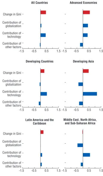
The results indicate that the main fac-tor driving the recent increase in inequality across countries has been technological prog-ress. Based on the benchmark model, which is described in more detail in Appendix ., technological progress alone explains most of the 0.5 percent average annual increase in the Gini coefficient from the early 980s (Table .,
column b; and Figure .9).27 Trade and
finan-cial globalization and finanfinan-cial deepening 25An additional advantage of focusing on within-country variation is to reduce the risk of omitted variable bias. The impact of common global shocks such as business cycles or growth spurts is excluded using time dummies.
26Since income and consumption surveys are not con-ducted annually, the estimations use an unbalanced panel with observations included only for years for which actual data are available. Moreover, given the smaller size of the samples for advanced and developing economies, the results on these subgroups are more tentative.
27The results are robust to including changes in GDP per capita as an explanatory variable. However, this vari-able was excluded in the reported estimations in order to estimate the full effects of the variables of interest, including their effect through higher overall growth. Other possible explanatory variables (democracy, constraints on the executive, flexibility of regulations, real exchange rate, and terms of trade) were initially included, but their effects were not robustly estimated. Comprehensive data on government social spending and transfers, migration, and remittances were not available across all countries, although these channels may poten-tially have important additional effects on the observed inequality outcomes.
Figure 4.9. Explaining Gini Coefficient Changes (Average annual percent change)
1,2
All Countries Advanced Economies
Developing Countries Developing Asia
Change in Gini Contribution of globalization Contribution of technology Contribution of other factors Change in Gini Contribution of globalization Contribution of technology Contribution of other factors
Latin America and the
Caribbean Middle East, North Africa, and Sub-Saharan Africa
Change in Gini Contribution of globalization Contribution of technology Contribution of other factors
Source: IMF staff calculations.
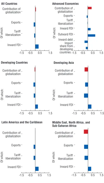
1981–2003 or longest subperiod for which all variables used in the regression are available. The contribution of each variable is computed as the average annual change in the variable times the regression coefficient on the variable (see Appendix 4.1). For the “All countries” panel, regression coefficients are taken from the full sample estimation in column (b) of Table 4.1. For the country group panels, regression coefficients are taken from Table 4.3, which provides group-specific estimates of the coefficients. See Figure 4.10 for the composition of the contribution of globalization. The contribution of other factors is the sum of the contributions of the ratio of credit to private sector to GDP, the education variables, the sectoral employment shares, and the residual.
1
2
The disequalizing effect of globalization was larger in advanced economies, in part because of outward foreign direct investment, while in developing countries, and especially in developing Asia, technological change was the main contributor to the rise in inequality. -1.5 -0.5 0.5 1.5 -1.5 -0.5 0.5 1.5 -1.5 -0.5 0.5 1.5 -1.5 -0.5 0.5 1.5 -1.5 -0.5 0.5 1.5 -1.5 -0.5 0.5 1.5