i
A NEAR REAL-TIME, HIGHLY SCALABLE,
PARALLEL AND DISTRIBUTED ADAPTIVE OBJECT
DETECTION AND RE-TRAINING FRAMEWORK
BASED ON THE ADABOOST ALGORITHM
By: Munther Abualkibash
Under the Supervision of Dr. Ausif Mahmood
DISSERTATION
SUBMITTED IN PARTIAL FULFILMENT OF THE REQUIREMENTS FOR THE DEGREE OF DOCTOR OF PHILOSOPHY IN COMPUTER SCIENCE
AND ENGINEERING THE SCHOOL OF ENGINEERING
UNIVERSITY OF BRIDGEPORT CONNECTICUT
iii
A NEAR REAL-TIME, HIGHLY SCALABLE, PARALLEL
AND DISTRIBUTED ADAPTIVE OBJECT DETECTION AND
RE-TRAINING FRAMEWORK BASED ON THE ADABOOST
ALGORITHM
iv
A NEAR REAL-TIME, HIGHLY SCALABLE, PARALLEL
AND DISTRIBUTED ADAPTIVE OBJECT DETECTION AND
RE-TRAINING FRAMEWORK BASED ON THE ADABOOST
ALGORITHM
ABSTRACT
Object detection, such as face detection using supervised learning, often requires extensive training for the computer, which results in high execution times. If the trained system needs re-training in order to accommodate a missed detection, waiting several hours or days before the system is ready may be unacceptable in practical implementations. This dissertation presents a generalized object detection framework whereby the system can efficiently adapt to misclassified data and be re-trained within a few minutes. Our developed methodology is based on the popular AdaBoost algorithm for object detection. AdaBoost functions by iteratively selecting the best among weak classifiers, and then combining several weak classifiers in order to obtain a stronger classifier. Even though AdaBoost has proven to be very effective, its learning execution time can be high depending upon the application. For example, in face detection, learning can take several days. In our dissertation, we present two techniques that contribute to reducing to the learning execution time within the AdaBoost algorithm. Our first technique utilizes a highly parallel and distributed AdaBoost algorithm that
v
exploits the multiple cores in a CPU via lightweight threads. In addition, our technique uses multiple machines in a web service similar to a map-reduce architecture in order to achieve a high scalability, which results in a training execution time of a few minutes rather than several days. Our second technique is a methodology to create an optimal training subset to further reduce the training execution time. We obtained this subset through a novel score-keeping of the weight distribution within the AdaBoost algorithm, and then removed the images that had a minimal effect on the overall trained classifier. Finally, we incorporated our parallel and distributed AdaBoost algorithm, along with the optimized training subset, into a generalized object detection framework that efficiently adapts and makes corrections when it encounters misclassified data. We demonstrated the usefulness of our adaptive framework by providing detailed testing on face and car detection, and explained how our framework applies to developing any other object detection task.
vi
ACKNOWLEDGEMENTS
In the name of God, the Most Gracious, the Most Merciful, I wholly devote my thanks to God who has helped me all the way to complete this work successfully. I owe a debt of gratitude to my loving family: my parents, my wife, Sawsan, and my daughters, Sarah and Lena, for all of their time waiting, and for their understanding and encouragement.
I am honored to have had the opportunity to work under the supervision of Dr. Ausif Mahmood. Throughout the course of this dissertation, Dr. Mahmood provided invaluable guidance, and worked tirelessly to help me craft this dissertation through several stages. His encouragement and support was vital to the completion of this dissertation.
I would like to express special thanks to Dr. Khaled Elleithy for his support, advice, and encouragement.
I would also like to express my gratitude to committee members Dr. Prabir Patra, Dr. Navarun Gupta, Dr. Miad Faezipour, and Dr. Saeid Moslehpour for their valuable feedback and discussion regarding this work.
I would like to thank Lydia Iarocci for assistance in proofreading and editing. Last but not least, I would like to thank all the staff of the School of Engineering for their support, who made my studies at the University of Bridgeport a wonderful and exciting experience.
vii
TABLE OF CONTENTS
ABSTRACT ... iv ACKNOWLEDGEMENTS ... vi LIST OF TABLES ... ix LIST OF FIGURES ... x 1 CHAPTER 1: INTRODUCTION ... 11.1 Research Problem and Scope ... 1
1.2 Motivation Behind the Research ... 4
1.3 Potential Contributions of the Proposed Research ... 5
2 CHAPTER 2: LITERATURE SURVEY ... 7
2.1 Introduction ... 7
2.2 The Concept of Boosting ... 7
2.3 AdaBoost Algorithm used by Viola and Jones ... 9
2.3.1 Integral Image ... 9
2.3.2 Extracted Feature Types and Selection ... 10
2.4 Previous Research on Parallel and Distributed AdaBoost ... 20
2.5 Previous Research on Training Classifiers on a Small Training Set ... 26
2.6 Summary ... 27
3 CHAPTER 3: RESEARCH PLAN ... 29
3.1 Parallel and Distributed Web Services-Based AdaBoost Architecture ... 29
3.1.1 Parallel Execution ... 32
3.1.2 Web Services and Parallel Execution on One-level Hierarchy ... 32
viii
3.1.4 Web Services and Parallel Execution on One-level Hierarchy with Number of Slave
Nodes ... 36
3.2 Extracting Minimum Size Subset that has 100% Detection Rate for Faces and Non-faces 38 3.3 Implementing a Cascade Structure Based on a Small Training Set ... 41
3.4 A Near Real-time Re-training ... 47
3.5 Summary ... 48
4 CHAPTER 4: RESULTS ... 49
4.1 Parallel and Distributed AdaBoost Testing Results ... 49
4.2 Pruning Techniques Testing Results ... 56
4.2.1 Pruning by Clustering ... 56
4.2.2 Pruning by Distance and Number of Neighbors ... 59
4.2.3 Pruning Using Recursive Elimination of Neighbors ... 60
4.2.4 Results of Pruning Techniques ... 62
4.2.4.1 Results of Pruning by Clustering ... 64
4.2.4.2 Results of Pruning by Distance and Number of Neighbors ... 65
4.2.4.3 Results of Pruning using Recursive Elimination of Neighbors... 66
4.3 A Near Real-time Re-training to Fix Results of Missed Objects and False Positives ... 67
4.3.1 The Proposed Framework Results for Cars ... 67
4.3.2 The Proposed Framework Results for Faces ... 74
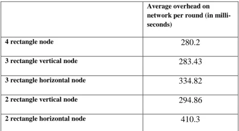
4.4 Power Analysis ... 78
4.5 Summary ... 86
5 CHAPTER 5: CONCLUSION ... 87
5.1 Future Directions ... 88
6 REFERENCES ... 89
ix
LIST OF TABLES
TABLE 2.1TOTAL NUMBER OF FEATURES USING 24X24 PIXELS WINDOW SIZE FOR LIENHART
AND MAYDT’S FEATURES [52] ... 13
TABLE 2.2EXAMPLE OF IMAGES AND LABELS ... 16
TABLE 2.3EXAMPLE OF IMAGES, LABELS, AND WEIGHTS... 16
TABLE 4.1COMPARISON OF THE FIRST FOUR APPROACHES USED ... 50
TABLE 4.2THE RESULT OF THE PREDICTIVE EQUATION BASED ON THE NUMBER OF NODES ATTACHED TO ONE SUB-MASTER NODE ... 52
TABLE 4.3OVERHEAD ON THE ONE-LEVEL NETWORK USING ONE MASTER AND 5 SLAVE NODES ... 52
TABLE 4.4OVERHEAD ON THE TWO-LEVEL NETWORK USING ONE MASTER,5 SUB-MASTER NODES, AND 25 SLAVE NODES ... 53
TABLE 4.5COMPARISON OF THE FIFTH APPROACH WITH DIFFERENT NUMBER OF NODES ... 54
TABLE 4.6EXAMPLE OF THREE IMAGES AFTER PRUNING BASED ON ID ... 64
TABLE 4.7EXAMPLE OF THREE IMAGES AFTER PRUNING BASED ON DISTANCE AND NUMBER OF NEIGHBORS ... 65
TABLE 4.8EXAMPLE OF THREE IMAGES AFTER PRUNING BASED ON RECURSIVE ELIMINATION OF NEIGHBORS ... 66
TABLE 4.9RESULTS OF RE-TRAINING TO DETECT A MISSED CAR ... 68
TABLE 4.10RESULTS OF RE-TRAINING TO DELETE FALSE POSITIVES ... 69
TABLE 4.11RESULTS OF DETECTING CARS BY THE PROPOSED FRAMEWORK WITHOUT RE -TRAINING ... 73
TABLE 4.12RESULTS OF RE-TRAINING TO DETECT A MISSED FACE ... 74
TABLE 4.13RESULTS OF RE-TRAINING TO DELETE FALSE POSITIVES ... 75
TABLE 4.14RESULTS OF DETECTING FACES BY THE PROPOSED FRAMEWORK WITHOUT RE -TRAINING ... 78
x
LIST OF FIGURES
FIGURE 2.1THE SUMMATION OF ALL PIXELS ON TOP AND TO THE LEFT OF X,Y IS THE
INTEGRAL IMAGE VALUE AT X,Y ... 9
FIGURE 2.2CALCULATING THE INTEGRAL IMAGE IN A RECTANGULAR REGION ... 10
FIGURE 2.3FIVE RECTANGULAR FEATURES.FIGURE (A) SHOWS TWO RECTANGLE HORIZONTAL AND VERTICAL FEATURES, FIGURE (B) SHOWS THREE RECTANGLE HORIZONTAL AND VERTICAL FEATURES, AND FIGURE (C) SHOWS A FOUR RECTANGLE FEATURE ... 11
FIGURE 2.4FEATURES (A, B, C, D, E, F, G, AND H) ARE EXAMPLES OF LINE FEATURES ... 12
FIGURE 2.5FEATURES (A, B, C, AND D) ARE EXAMPLES OF EDGE FEATURES ... 13
FIGURE 2.6FEATURES (A AND B) ARE EXAMPLES OF CENTER-SURROUND FEATURES ... 13
FIGURE 3.1ONE-LEVEL HIERARCHY FOR WEB SERVICES AND PARALLEL ADABOOST, BASED ON ONE MASTER AND FIVE SLAVE NODES (TOTAL OF SIX PCS) ... 30
FIGURE 3.2TWO-LEVEL HIERARCHY FOR WEB SERVICES AND PARALLEL ADABOOST, BASED ON ONE MASTER, FIVE SUB-MASTER NODES, AND 3 SLAVE NODES FOR EACH SUB -MASTER NODE (TOTAL OF TWENTY ONE PCS) ... 31
FIGURE 3.3ONE-LEVEL HIERARCHY FOR WEB SERVICES AND PARALLEL ADABOOST, BASED ON ONE MASTER AND N SLAVE NODES ... 31
FIGURE 3.4EXTRACTING AN OPTIMIZED TRAINING SUBSET ... 39
FIGURE 3.5EACH FEATURE VALUE IS CALCULATED IN EACH IMAGE FROM THE OPTIMIZED SUBSET OF THE TRAINING SET ... 40
FIGURE 3.6FINDING THE MULTIPLIERS FOR THE SUM OF ALPHAS ... 43
FIGURE 3.7MULTIPLIER COEFFICIENT FOR EACH STAGE TO ACHIEVE 100% TRUE POSITIVE DETECTION ... 44
FIGURE 3.8CLASSIFIER OF TWENTY ONE STAGES ... 44
FIGURE 3.9ARCHITECTURE FOR THE RE-TRAINABLE SYSTEM ... 48
FIGURE 4.1PARALLEL EXECUTION TIME BASED ON THE TOTAL NUMBER OF SLAVE WORKSTATIONS ... 50
FIGURE 4.2REAL AND PREDICTIVE PARALLEL EXECUTION TIME BASED ON TOTAL NUMBER OF SLAVE WORKSTATIONS IN THE LAST LEVEL ... 51
FIGURE 4.3PARALLEL EXECUTION TIME BASED ON THE TOTAL NUMBER OF SLAVE WORKSTATIONS USING THE MASTER –N SLAVE NODES APPROACH ... 54
xi
FIGURE 4.4REAL AND PREDICTIVE PARALLEL EXECUTION TIME BASED ON THE TOTAL
NUMBER OF SLAVE WORKSTATIONS USING THE MASTER –N SLAVE NODES APPROACH
... 55
FIGURE 4.5MULTIPLE RECTANGLES ON EACH FACE AND SOME FALSE POSITIVE RECTANGLES ... 56
FIGURE 4.6EACH 1-VALUE REPRESENTS A RECTANGLE IN THE REAL IMAGE IN FIGURE 4.5 ... 57
FIGURE 4.7A UNIQUE ID FOR EACH GROUP OF 1-VALUES ... 57
FIGURE 4.8THE 8 NEIGHBORS OF THE CENTER POINT ... 58
FIGURE 4.9(A, B, C) EXAMPLE OF THREE IMAGES USED FOR TESTING ... 63
FIGURE 4.10(A, B, C) EXAMPLE OF THREE IMAGES AFTER DETECTING THE EXPECTED FACES AND FALSE POSITIVES ... 63
1
1
CHAPTER 1: INTRODUCTION
1.1 Research Problem and Scope
Object detection is an important area of research in computer vision. One of the most popular approaches for object detection is based on combining many weak classifiers together to achieve one strong classifier through a technique called Boosting. A modified version of this technique was developed by Viola and Jones, where a classifier is created by iteratively selecting a best single feature (weak) classifier from a set of a very large number of potential features. If a sequential implementation is used for boosting, it becomes a time consuming process often requiring days of execution time to implement a classifier with a reasonable number of features. Thus, an efficient parallel boosting algorithm is highly desired for object detection [1].
Boosting has been applied to various object detection implementations such as face [2], car [3-5], and airplane detection [6]. Of these, face detection has received considerable attention as it has proven to be a more challenging field. Also, face detection is needed in many practical applications, such as intelligent human-computer interfaces, video conferencing, and face recognition. For face recognition, first, faces need to be detected by finding their locations in the image, then the faces are extracted, before finally performing the recognition [7].
2
Many approaches have been developed to detect faces in the last couple of decades. Some of these are based on statistical learning methods, e.g., Support Vector Machine [8], Neural network [9], and Bayesian decision rule [10]. Hjelmas and Low [11] and Yang et al. [12] provide surveys of most of the face detection approaches prior to 2002. Based on Yang et al.’swork, face detection approaches can be classified into four major categories: first, the knowledge-based method in which human knowledge is the basis for face determination; second, the feature invariant approach that makes finding the structure of facial features easy, even in difficult conditions such as strong lighting; third is the template matching method, which focuses on the storing of faces for matching purposes; finally, the appearance-based method that trains the computer to detect faces. Of these, the appearance-based approach yields better results but requires more processing. Since the speed of computers is continuously increasing, using appearance-based methods is preferred compared to the other methods. One of the most significant contributions to face detection work in the appearance-based category is from Viola and Jones [2, 13, 14]. The original Viola and Jones algorithm was published in 2001, and since then it has become the most popular approach to face detection because of its high accuracy and real-time detection capabilities.
Another survey in 2010 by C. Zhang and Z. Zhang [15] discusses the new enhancements in face detection since the previously published surveys of [11] and [12] in 2001 and 2002 respectively. Their main focus is on face detection through boosting algorithms. One of the examples of detecting faces through boosting has been done by Viola and Jones [2, 13, 14]. Viola and Jones’ algorithm is based on a variation of boosting technique called AdaBoost [16], short for Adaptive Boosting, which employs a
3
concept called integral image that greatly reduces the number of computations in the detection algorithm. Furthermore, it uses a cascade of classifiers in an effective manner to obtain high real-time face detection accuracy.
Since AdaBoost is resistant to overfitting [17, 18] and Viola and Jones’ algorithm [2, 13, 14] has proven itself to be accurate and fast at the same time, the purpose of this work is to focus on improving this approach by developing a framework that can adapt efficiently to false positives and false negatives in object detection in real implementations through a highly parallel and reduced optimized dataset re-training process. Learning from a smaller training dataset has the important advantage of better generalization in addition to reduced re-training execution time. When the system is able to obtain good classification results through a small number of training examples, this itself is strong proof of the system’s generalization abilities [19].
In this dissertation, in order to develop an adaptive near real-time and re-trainable object detection framework, a new parallel and distributed implementation of the AdaBoost boosting algorithm has been proposed and developed. The implementation of the proposed parallel AdaBoost not only reduces the execution time, it also requires less memory for the distribution of training samples to processing nodes. The memory requirement is further reduced by requiring fewer training samples. This has a positive effect on the execution time, as the entire training dataset can be easily stored in the main Random Access Memory (RAM), eliminating the disk swapping that usually occurs in a traditional AdaBoost implementation when the standard set of training samples is used, as provided by Viola and Jones. To exploit the parallelism at the multi-core level for this object detection framework, the Task Parallel Library (TPL) has been used. To further
4
reduce the execution time, the process incorporates distributed processing on a network of workstations through the use of web services. Even though parallel or distributed implementations of AdaBoost have been reported (e.g., [1, 20-37],) none of the existing parallel approaches matches this proposed implementation in terms of its efficiency in its execution time. This is mainly because the parallel approach is multifaceted; that is, it employs distributed processing in terms of web services and its highly parallel multi-core exploitation through TPL, and reduces memory usage through distribution and optimization of the training dataset.
1.2 Motivation Behind the Research
These days, there are many algorithms for object detection; however, none of them have a 100% detection rate. Therefore, better algorithms are needed so that the detection rate can be near 100% and false positives can be reduced. At the same time, it is also challenging to provide a high detection rate in real-time. Usually, training a classifier might take several days to learn to detect objects, and the difficulty in training a base classifier is known to be a computational problem [38, 39].
However, in cases where the system failed to detect a valid object, there should be a methodology where the system can be re-trained instantly so that such false negatives can be avoided. For example, where a face detection system is installed in a site, if an employee has a change in facial appearance because of an injury or changing hair styles, the system might fail to detect their face. In such cases, there is a need for a system that can be re-trained to adapt to changing features in near real-time. As a result, building a
5
framework able to re-train a classifier to take care of missed examples of an object, as well as to reduce the number of false positive examples, is highly needed.
This research is motivated by the drawbacks and limitations of existing systems, as well as the following reasons:
First, the AdaBoost algorithm [2, 13, 14] is one very famous approach in the object detection field. Second, to make the AdaBoost algorithm more useful, a huge amount of computation power is needed. Third, multi-core processors have become very common and effective in using multiple threads simultaneously, which greatly enhances computational power. Multi-core processors are the best suited to computer vision algorithms because of their high computational power and multi-threading features. Parallel and distributed AdaBoost can be used to speed up the training process in cases where a classifier must be trained in a very short time. For example, supposing there is a need to train a face detector on a client site, the system needs to be customized to the site’s specific conditions. In such cases, it is highly desirable that the training phase can be done as quickly as possible.
1.3 Potential Contributions of the Proposed Research
We develop a novel, highly parallel and distributed implementation of the Viola and Jones algorithm that exploits the multiple cores in a CPU via lightweight threads, and also uses multiple machines via web service software architecture, to achieve high scalability. Based on the number of processors available, a nearly linear increase in processing speed is achieved, and the learning of a feature in the AdaBoost algorithm can be accomplished within a few seconds. The training execution time is further reduced by
6
using a smaller optimized training dataset. The features extracted from this small optimized subset achieve a high detection rate. The significant speedup of the proposed parallel and distributed AdaBoost enables us to extract the optimized subset from the entire set. The optimized subset is yielded by replacing some images with other images based on the weight value assigned by the AdaBoost algorithm, until getting a small subset that can achieve high detection rates. We encapsulate the entire parallel and distributed system into a general object detection framework where the training dataset can be updated as a result of misclassified data, and the system re-trained within a few minutes. Therefore, this general object detection framework is considered an adaptive framework such that a smaller optimized training subset is used to yield high detection rates while further reducing the re-training execution time. We demonstrate the usefulness of our adaptive framework on face and car detection. The framework developed here is applicable to any object detection task.
7
2
CHAPTER 2: LITERATURE SURVEY
2.1 Introduction
There have been many attempts to speed up the AdaBoost algorithm. The following are two main approaches to speed up AdaBoost: (1) reducing the number of data points that participate in training the base learners or (2) reducing the search area by using only a small set of features [1]. In order to speed up AdaBoost more quickly, there is a way to use both approaches together: by using less data and fewer features, a significant reduction in computation time can be observed.
2.2 The Concept of Boosting
Boosting is a well-known ensemble learning method based on the concept that a strong classifier will be produced if repetitive enhancements are applied to any weak base-learner. The concept of boosting evolved from the theoretical question of whether one strong classifier can emerge from any weak learning classification tool. This concept was proven through the development of the first boosting algorithms by Schapire [40] and Freund [41].
Where a binary classification exists, the rate of accurate classification from a weak learner is somewhat higher than the rate from a random guess, while a strong
8
learner should obtain an almost completely accurate classification. In theory, the process of obtaining a strong learner is difficult in comparison to obtaining a weak learner [42].
Boosting algorithms learn by obtaining an accurate classification through iteratively merging weak learners. The concept of boosting was mentioned by Schapire and Freund in [43], where the classification of each base-learner achieves a somewhat better result than random guessing, because each base-learner has some useful information about the problem structure. However, there would be no difference in the weak learner’s performance by only repeating it several times on the same training set [44]. In boosting, the base-learner performance is improved by not only handling the base-learner itself, but by iterative re-weighting of the training set [43]. Therefore, the base-learner will obtain a different result from the information in every loop.
The success of the base-learner in one round will play a main role in objects’ weighting in the next round. As a result, misclassified objects will receive more concentration by being assigned higher weights.
The precision in boosting is yielded by incrementally raising the importance of the objects that are hard to classify. For each round, the weights are calculated based on the successful classification results of prior rounds. During each round, all misclassified objects from previous rounds will receive more attention. At the last stage, one accurate prediction is created by putting together all the outputs of the prior base-learners [44].
Another well-known ensemble learning method is called bagging [45]. The name baggingwasderivedfrom“bootstrapaggregation”.Itwasoneoftheeasiestapproaches to improving classification by using multiple samples from one data set.
9
At the beginning, bagging was used for decision tree models; however, it can also be applied for classification or regression. In the bagging approach, many different training set versions are used, where each set is applied to the training of a different model. In a regression situation, the results of the models are combined by averaging. However, in a classification situation, the results are combined by voting to generate one result. When a small modification occurs in the training set, then a serious change can happen in the model. As a result, Bagging is more successful in unstable nonlinear models [44, 46].
2.3 AdaBoost Algorithm used by Viola and Jones
One of the main contributions of Viola and Jones is the integral image [2, 13, 14]. The benefit of using the integral image is to speed up the computation of rectangular features used in AdaBoost. This section reviews the calculations in the integral image and describes the AdaBoost algorithm.
2.3.1 Integral Image
To get the integral image position values x, y, the summation of the all pixel values located above and to the left of x, y is taken. Figure 2.1 explains this concept.
10
The following equation explains the computations for the integral image:
where represents the integral image value, and represents the original image value.
Figure 2.2 Calculating the integral image in a rectangular region
For obtaining the integral image value for the dark rectangle in Figure 2.2, integral image values of points 1, 2, 3, and 4 are calculated for the following equation:
2.3.2 Extracted Feature Types and Selection
The features extractedin ViolaandJones’algorithm arebasedonHaarfeatures [2, 13, 14, 47]. By applying integral images, calculation of Haar features can happen in a constant time [48].
A further advantage of Haar features is the power of the features in dealing with lighting variance and noise. Subtracting the difference between the dark and light sides of the rectangle prevents the impact of noise and lighting variance, which would affect all
11
the pixel values of the entire image equally [49]. Another advantage of Haar features is the easiness of altering the scale of the features [50].
The five types of Haar features used in the original algorithm are shown in Figure 2.3.
Figure 2.3 Five rectangular features. Figure (a) shows two rectangle horizontal and vertical features, figure (b) shows three rectangle horizontal and vertical features, and figure (c) shows a four rectangle feature
To calculate the value of an image based on a particular feature (feature value), the sum of the integral image values for the pixels located in the light side of the rectangle are subtracted from the dark side [2, 13, 14]. The window size used for training and detecting purposes in face detection is 24x24 pixels. For scaling, the starting point is the smallest size of a rectangular feature, e.g., in a three rectangle feature type, it is 3x1 pixels; in a two rectangle feature type, it is 2x1 pixels. Each rectangular feature is scaled up until reaching a total window size of 24x24. As a result, the total number of features for each type is:
For a three rectangle feature type, 27,600 features For a two rectangle feature type, 43,200 features For a four rectangle feature type, 20,736 features
The total number for all features combined is: three rectangles horizontal + three rectangles vertical + two rectangles horizontal + two rectangles vertical + four rectangles = 27,600 + 27,600 + 43,200 + 43,200 + 20,736 = 162,336 features. During the learning
12
phase, all of these features will be computed for all faces in the training set. The set of faces used for training purposes in this study is the same one that has been used by Viola and Jones for face detection [2, 13, 14]. The size of each image is 24x24. There are 4,916 faces and 7,960 non-faces in the set [51]. Thus, the total number of all possible features in all training images is 2,090,238,336 (i.e. number of training images multiplied by features per image).
Lienhart and Maydt [52] added a set of 45° rotated Haar features, which improve the basic set of Haar features that was used by Viola and Jones, and which can also be computed in an efficient way in constant time at all scales. In addition, the extended set adds extra domain-knowledge to the training phase, which is tough to learn. Lienhart and Maydt mentioned that by employing these extra rotated Haar features, the false alarm rate decreased by about 10% at a specific hit rate.
14 feature prototypes were added by Lienhart and Maydt, which are divided into three different groups: eight line features, four edge features, and two center-surround features, as shown in Figure 2.4, Figure 2.5, and Figure 2.6.
Eight line feature prototypes
Figure 2.4 Features (a, b, c, d, e, f, g, and h) are examples of line features
13
Four edge feature prototypes
Two center-surround feature prototypes
After applying only the features that were not used by Viola and Jones on window size 24x24, the total number of features obtained after scaling is shown in Table 2.1.
Table 2.1 Total number of features using 24x24 pixels windowsizeforLienhartandMaydt’sfeatures[52]
Line features Number of features
a 20,736
c 20,736
e 4,356
Figure 2.5 Features (a, b, c, and d) are examples of edge features
a b c d
a b
14
f 4,356
g 3,600
h 3,600
Edge features Number of features
a 8,464
b 8,464
Center-surround features Number of features
a 1,521
b 8,464
Total 84,297
Lienhart and Maydt’s features were not implemented in this dissertation. However, adding the features that were used by Lienhart and Maydt (a total of 84,297 features) to the features that were used by Viola and Jones (a total of 162,336) would result in using a total of 246,633 features, which would increase the training time to find the best feature among total features.
15
Viola and Jones have used AdaBoost to select features and combine weak classifiers into one strong classifier [53]. Peter Harrington [54] has mentioned that “AdaBoostisconsidered by some to be the best supervisedlearningalgorithm.”
The conventional AdaBoost algorithm used by Viola and Jones works by assigning a weight to each image in the training set, where all images have an equal weight at the beginning. Training is started on the training set to obtain a first weak classifier and calculate the error of this weak classifier. Next, the weights of all images in the training set are adjusted based on the error, where falsely classified images are assigned a relatively higher weight. Then, the second weak classifier is trained based on the new updated weights [2, 13, 14, 54]. The training will be repeated to extract more weak classifiers, and the weights will be adjusted on every iteration until reaching the maximum number of iterations that is assigned by a user.
As a result, each α value for every weak classifier is determined based on the error value (ɛ) of that weak classifier, where each error value is calculated by dividing the number of misclassified images over the total number of images [54].Therefore,αvalue is calculated as seen in the following equation:
The main goal of a weak classifier is to get the optimal threshold among positive and negative examples for any rectangular feature. This technique has been known as the decision stump, which is considered a simple decision tree [55]. The pseudocode of implementing the decision stump, using the indexes of the sorted values of the features to accelerate the process, is explained later in this chapter. The selected threshold minimizes
16
the number of misclassified examples. The decision of a weak classifier is 1 or 0, i.e. positive or negative, as shown in the following equation:
where p is either 1 or -1, is the threshold, and f is the feature. Pseudocode of the AdaBoost algorithm:
Suppose there are N number of images in a training set. Each image is labelled as
either 0, for negative images, or 1, for positive images, as shown in Table 2.2
Table 2.2 Example of images and labels Images
Label 1 0 0 1
Initializing the weight for each image in the first round is shown in the following
table:
Table 2.3 Example of images, labels, and weights
Images
Label 1 0 0 1
Weight
where l is the total number of positive images (i.e. faces) and m is the total number of negative images (i.e. non-faces) in the training set
For t = 1 to T:
17
=
, where is the sum total of the weights of all images in the same round.
2. Calculate the error of all features, until finding the feature that has the minimum error. The selected feature is the best weak classifier in round
=
3. Based on the minimum error , which is determined by , find
4. As preparation for the next round, the weight should be updated:
where if is misclassified, otherwise, and =
At the end, after going through all rounds, the strong classifier is determined as
follows: where =
18
Pseudocode of the decision stump 1. Setminimum_error=+∞ 2. Set threshold = 0 3. Set sign = 0 4. Set current_error = 0 5. Set e_p = 0 6. Set e_n = 0 7. Set epsilon = 0 8. Set index = 0 9. Set h_classification = 0
10.Set total_error = summation of the weight of all images
11.Set negative_weights_sum = summation of the weight of all negative images only 12.Set positive_weights_sum = summation of the weight of all positive images only 13.Set negative_weights_sum_below = negative_weights_sum
14.Set positive_weights_sum_below = positive_weights_sum 15.For 1... Total number of images
Set index = the index of the image in the images list as ordered by the feature value
If the label of the current image in the loop returned by index presents a positive label
Subtract the weight of that current image from positive_weights_sum_below
19
Subtract the weight of that current image from negative_weights_sum_below
Set e_p = positive_weights_sum_below + (negative_weights_sum - negative_weights_sum_below)
Set e_n = negative_weights_sum_below + (positive_weights_sum - positive_weights_sum_below)
If e_p < e_n
Set current_error = e_p
If minimum_error > current_error Set minimum_error = current_error
Set threshold = the feature value of the current image Set sign = -1
Else
Set current_error = e_n
If minimum_error > current_error
Set minimum_error = current_error
Set threshold = the feature value of the current image Set sign = +1
16.For 1... Total number of images
If the feature value of the current image in the loop > threshold Set h_classification = sign
20
Set h_classification = sign * -1
If h_classification value does not match the label of the current image in the loop Set epsilon = epsilon + the weight value of the current image in the loop 2.4 Previous Research on Parallel and Distributed AdaBoost
Some AdaBoost algorithms that were mentioned in the literature paid more attention to enhancing the generalization error or the degree of toughness when it dealt with noisy data [23, 56, 57]. Additionally, different attempts have been made to parallelize AdaBoost to speed up learning time. K. Zeng et al. [25] parallelized AdaBoost through the hybrid usage of MPI, OpenMP, and transactional memory. By sharing data through transactional memory, OpenMP has been used for low level parallelization and MPI for high level parallelization. K. Zeng et al. [25] built a heterogeneous PC cluster system of sixteen PCs using two processor types. PCs with the same processor type were grouped. In one group, there are 8 PCs with Core2 Quad 2.8G processors and in the other group there are 8 PCs with Core2 Dual 2.8G processors. Each group has the PCs connected to each other through 100Mb Ethernet. The total number of images in the set includes 64,328 faces and 43,712 non-faces. The size of each image is 20x20 pixels, and the total number of Haar features is 299,298. Their AdaBoost algorithm ran for 1,000 rounds. K. Zeng et al. [25] reported a speedup of 31.2 over a sequential implementation with 48 cores. In our implementation where we used the Intel Xeon Quad-Core Processor E5-1620 3.6GHz and a RAM size of 16 GB, the speedup obtained was 44.5 when using 48 cores.
21
Another attempt was made by Lazarevic and Obradovic [26] to solve the problem of learning an enormous homogeneous database for training classifiers by distributing the database over many places. The database size was too large to fit in one place, preventing it from being located in the computer memory. Also Lazarevic and Obradovic [27] parallelized AdaBoost using a database that was distributed because of the enormous size of the datasets. Their approach is based on dividing the data into separate small sets to use each set later in training base classifiers. Outputs of these classifiers are then combined based on their accuracy. Their parallel boosting algorithm is capable of working on a distributed database; however, it is not suitable to work in environments such as distributed cloud computing since their architecture relies on the shared memory systems technique. In addition, Merler et al. [28] used weight dynamics to parallelize AdaBoost and named it P-Adaboost. It is noticed that the outputs of these three previous parallel AdaBoost algorithms [26-28] do not match the sequential AdaBoost outputs because the authors made some changes to the training process of the original version of AdaBoost. However, K. Zeng et al. [25] found the same output for both parallel and sequential AdaBoost. Idealy, there should be no differences in the output of parallelized AdaBoost and sequential AdaBoost except to reduce the training time.
Galtier et al. [29] used JavaSpace and MPJ to parallelize AdaBoost where the output of parallel AdaBoost is same as in the sequential one. Because of hierarchical hardware architecture, K. Zeng et al. used the hybrid programming model. However, Galtier et al. [29] used the message passing model. In addition, Galtier et al. [29] parallelized AdaBoost by distributing balanced load tasks to multiple workers. Their
22
work is based on heterogeneous processors in a geographically distributed environment. However, this kind of setup produces latency on the network. The authors mentioned that using virtual shared memory in large distributed locations did not prevent them from speeding up the process in many cases.
Galtier et al. [29] used 134,736 Haar features with a training dataset of 8,500 24x24-pixel images. The speedup obtained with 64 workers on a homogenous cluster was 53.9 as compared to their sequential implementation. In our algorithm, the total number of Haar features is much higher (i.e. 162,336) and the training dataset size is also larger (12,876 images of 24x24 pixels). Despite the large dataset and feature sizes, using 64 cores, we obtain a speedup of 55.7 and much less execution time per feature.
Palit and Reddy [1] used parallel AdaBoost to get a boosted ensemble classifier by using the computation process in many nodes working at the same time. This resulted in a better performance as compared to using the serial version of AdaBoost, and they were able to speed up computation time. One of the reasons for this is that each one of the nodes used for computation purposes works individually, where there is no data shared between nodes. As a result, there is no communication occurring between nodes. The basic structure of their parallel algorithm does not follow the basic structure of the serial version of AdaBoost. Palit and Reddy implemented and tested their parallel algorithm using the MapReduce framework. Their approach makes the computation process of each node independent from the other nodes in order to reduce the communication cost between nodes.
23
Another approach for speeding up AdaBoost, called LazyBoost, was done by Escudero et al. [30], which takes advantage of using different feature selection and ranking methods by training the base learner in each boosting iteration on a random small set of features of a selected fixed size. Another fast boosting algorithm has been developed by Busa-Fekete and Ke´gl [31] that uses multiple-armed bandits (MAB). In MAB, there are many small groups of the base classifier sets thatareconsidered“arms”. Therefore, in each boosting iteration, there is only one small set among all the small sets that will be chosen to be used by the boosting algorithm, instead of training the base classifier using all the sets. However, the work to speed up AdaBoost mentioned in [30, 31] was done on a single machine, and a parallel and distributed architecture was not applied; therefore, their achievement was bounded by the resources of the single machine used.
There is another approach in boosting parallelization, where the parallelization occurs in the weak learner instead of parallelizing the ensemble itself. Wu et al. [32] used MapReduce to create an ensemble of C4.5 classifiers, and they called it MReC4.5. To enable the classifiers to be used in different environments, they have to be established in the cloud or on cluster computers, and any operations on serial form should be sequenced at the model level.
Another framework built using MapReduce on a large data set for regression trees and learning classification purposes was done by Panda [33], and is called PLANET. However, the previous approaches [32, 33] cannot be generalized to be used in boosting ensemble methods, since they are mostly limited to use for weak learners.
24
In another parallelizied boosting algorithm, Fan et al. [34] implemented a scalable and distributed learning type of boosting algorithm. Among the entire training set, only a small part is used to train each different classifier. Two different ways have been used to train the classifiers: either using random samples (r-sample), or the entire training set is disjointed into separate small sets (d-sample) so that on every round, the weak learner will receive a different d-sample. The main focus of the approach in Fan et al. [34] was parallelization in space, not in time. By distributing massive data on multiple nodes, the space problem was handled. However, gaining faster speed in processing time had not yet been reached.
Another algorithm called the MultBoost algorithm was proposed by Gambs et al. [35]. It was basically created to accomplish computation privacy. The design of the MultBoost algorithm enables it to work in a parallel setting. However, it can be parallelized in both space and time if each node has independent data, and if the computation process of each node is totally isolated, and does not know or rely on other nodes’data. In the MultBoost algorithm, two or more nodes are able to start a boosting classifier in a privacy-preserving setting.
Huang and Shi [24] implemented a parallel and distributed AdaBoost. All the features that were used in AdaBoost training were divided into multiple feature blocks, where the structure of the feature block is based on three components: block number, basic data, and optimal feature of that block. The distributed system is based on client computers and a server pool, where all the computing nodes are in the server pool. In Adaboost, there are sequential and parallel parts; the client is responsible for the
25
sequential part, and all the parallel parts will be sent to the computation nodes. Once each node completes the assigned task, the output will be sent back to the client to combine it and produce the final result. Huang and Shi used 5,646 face and 13,030 non-face images collected from the Internet as a training set, and the size of each image was 20x20 pixels. They tested their parallel algorithm on 5 PCs where the CPU speed was 1.8GHz on each PC. The maximum obtained speed based on extracting 64 features was 2.66 times faster compared to their implementation of the sequential AdaBoost algorithm. However, using N nodes did not allow them to reach the ideal value of N times because the weights were updated in each iteration, which could not be parallelized. Also, they were not able to save that huge number of features in the memory simultaneously, which led to longer training.
Lozano and Rangel [36] worked to speed up boosting algorithm running time by changing the training process of the base learners from sequential to parallel. However, they accomplished boosting parallelization on different algorithms equivalent to AdaBoost, where several individual distributions of the data were used to train many base learners concurrently before combining them. Their algorithm is executed in batches, where the first batch works like bagging [37]. Probability simplex was used to obtain random individual distributions to train base classifiers. Different approaches were then implemented in the subsequent batches, which depended on the information generated from the execution of the base learners in the prior batches, in order to get a useful distribution. One main processor rapidly generated all these distributions and then sent them to individual processors to obtain a new trained batch of base learners. Lozano and
26
Rangel focused on methods more than performance and implementation problems. However, Galtier et al. [29] paid more attention to performance and implementation problems. Lozano and Rangel’s [36] approach is different as compared to Lazarevic and Obradovic’s [27] approach in that the whole data set is used to train the base learner of every processor [36].
2.5 Previous Research on Training Classifiers on a Small Training Set
Freund and Schapire [16] mentioned that it is possible to train a base learner using only a small set of randomly selected data instead of using the entire weighted data, by using the weight vector as a discrete probability distribution.
FilterBoost [58] is an algorithm for using a small set to train a base learner. It is based on the modification [59] of AdaBoost aimed at reducing the logistic loss. In every boosting iteration while using the FilterBoost algorithm, many labeled samples are generated. However, the base learner has the choice to accept or reject the generated sample point, and among the accepted points, only a small set is used in the base learner training process.
C. Shen et al. [60] proposed an approach to training classifiers to detect faces based on a small training set by using covariance features [61] instead of Haar features, and Fisher Discriminant Analysis (FDA) instead of decision stump.
After Viola and Jones [2] developed real-time face detection based on AdaBoost, much has been done to improve their work either by enhancing the boosting method or by speeding up the training process; for example, S. Z. Li and Z. Zhang [62] presented an enhanced FloatBoost method that enhances detection accuracy by using backward feature
27
selection in AdaBoost training. J. Wu et al. [63] accelerated the training process by using forward feature selection. P. Minh-Tri and C. Tat-Jen [64] used approximation to decrease the training time when using the decision stump.
X. Li et al. [65] combined active learning with AdaBoost to increase the classification performance of AdaBoost while using a small sample set for training. AdaBoost is applied to the current labeled sample set to get an optimal hyperplane, and selecting any unlabelled sample that is closest to the optimal hyperplane. One of the drawbacks of using active learning is the risk of uninformative examples, which overwhelm the active learning algorithm.
K. Levi and Y. Weiss [19] worked on training classifiers to detect objects based on small training sets. However, their features were presented using local edge orientation histograms (EOH) instead of Haar features.
2.6 Summary
Using both a smaller amount of data and features by reducing the number of data points that participate in training the base learners, and reducing the search area by using only a small set of features will result in a significant reduction in computation time, when compared to using only one of these methods.
There is another way of training classifiers by using online learning [66] instead of offline learning, which the majority of training processes do. N. C. Oza [66] proposed an online version of bagging and boosting. The way online learning algorithms work is by dealing with every single example of a training set as it arrives. Therefore, no example of the training set will be saved or reused. Regarding the speed of such an online
28
algorithm, N. C. Oza has mentioned that “such algorithms run faster than typical batch algorithms in situations where data arrive continuously. They are also faster with large training sets for which the multiple passes through the training set required by most batch algorithms are prohibitively expensive.” [66]
The critical part in online learning is the computation process of sample weights, because there is no previous knowledge about how difficult the sample is. As a result, an estimation of the importance of the sample is necessary while this sample goes through every base classifier [67].
Since our proposed framework is based on parallel AdaBoost and web services, and uses an optimized training set, memory is not a problem as in other cases. For now, there is no need to use online learning because of parallel and distributed offline learning.
29
3
CHAPTER 3: RESEARCH PLAN
3.1 Parallel and Distributed Web Services-Based AdaBoost Architecture
This chapter presents the implementation of the proposed framework in parallel and distributed AdaBoost. The original AdaBoost determines the best weak classifier in each round based on the minimum classification error. The AdaBoost algorithm must go through all features to determine which feature yields the minimum error. Since there is a large number of features, the execution time during the learning phase is high. Our parallel approach [68] speeds up the execution time by efficiently parallelizing the AdaBoost algorithm. We implement a four-way approach in order to get results in the shortest possible time. We run the main computational part of AdaBoost in parallel, using Task Parallel Library (TPL). Task Parallel Library is a library built into the Microsoft .NET framework. The advantage of using TPL is apparent in multi-core CPUs where the declared parallel workload is automatically distributed between the different CPU cores by creating lightweight threads called tasks [69].
To further improve the execution time of AdaBoost, we use web services to run parallel Adaboost on multiple workstations in a distributed manner. Our first-level architecture does workload division based on feature type. Since there are five feature
30
types, we use five workstations at Level 1. As shown in Figure 3.1, a total of six machines are used, one master and five slave nodes. To achieve further scalability, computation of each of the feature types is further expanded to a second level using web services. Figure 3.2 illustrates twenty-one PCs being used in a two-level hierarchy: master, sub-masters, and slave nodes. Figure 3.3 shows number of PCs being used in a one-level hierarchy: master and slave nodes.
Figure 3.1 One-level hierarchy for Web Services and Parallel AdaBoost, based on one master and five slave nodes (total of six PCs)
31
Figure 3.2 Two-level hierarchy for Web Services and Parallel AdaBoost, based on one master, five sub-master nodes, and 3 slave nodes for each sub-sub-master node (total of twenty one PCs)
Figure 3.3 One-level hierarchy for Web Services and Parallel AdaBoost, based on one master and N slave nodes
The following list consists of four approaches for speeding up execution times that are implemented in the AdaBoost algorithm:
Parallel execution
Web Services and Parallel execution on one-level hierarchy Web Services and Parallel execution on two-level hierarchy
32
Web Services and Parallel execution on one-level hierarchy with number of slave
nodes
3.1.1 Parallel Execution
All features are grouped based on type, such as three rectangle horizontal, three rectangle vertical, two rectangle horizontal, two rectangle vertical, and four rectangle. Each group is uploaded to the system memory in parallel. Once all of these have been loaded, the AdaBoost rounds from 1 to T begin. For each round, the result is to locate five features that have minimal error, in parallel, from five different groups. Among the five selected features, the feature that possesses the least minimum error is chosen. From that selected feature, the weights of all images are updated in preparation for the next round of the AdaBoost algorithm. One advantage of the previous mentioned approach lies within its execution time. Since selecting a minimum error feature runs simultaneously, the execution time is reduced by approximately a factor of five.
3.1.2 Web Services and Parallel Execution on One-level Hierarchy
Each group of features is distributed to a separate PC. Since five groups exist, five PCs are used for feature calculations, and the master coordinates the five PCs as shown in Figure 3.1. The parallel and distributed pseudocode for this approach is described below.
Pseudocode of one-level hierarchy (master and five slave workstations) Parallel and Distributed AdaBoost:
33
1) Example images where for negative and positive examples, respectively, are given
2) Prepare one master workstation and five slave workstations 3) Each slave workstation is assigned to one particular feature type
(slave workstation 1, Three rectangles Horizontal) (slave workstation 2, Three rectangles Vertical) (slave workstation 3, Two rectangles Horizontal) (slave workstation 4, Two rectangles Vertical) (slave workstation 5, Four rectangles)
4) On slave workstations: Initialize all images on each slave workstation 5) On master workstation:
Initialize weights for respectively, where and are the
number of negatives and positives, respectively For
1. Normalize the weights,
so that is a probability distribution 2. Send the weights to all slave workstations
3. On each slave workstation:
a. For each feature , train a classifier h which is restricted to using a single feature. The error is evaluated with respect to = h b. Send the classifier h with the lowest error to master workstation 4. On master workstation:
34
a. Among the received classifiers from each slave workstation, choose the classifier h with the lowest error
b. Update the weights: = where if example is
classified correctly, otherwise , and
6) The final strong classifier is:
h h
h
where
3.1.3 Web Services and Parallel Execution on Two-level Hierarchy
The previous technique divided the work based on feature type. Now, we further distribute the calculations in a feature type to another set of machines in the next hierarchical level as shown in Figure 3.2.
Pseudocode of two-level hierarchy (master, five sub-master workstations, and 25 slave workstations) Parallel and Distributed AdaBoost:
1) Example images where for negative and positive examples, respectively, are given
2) Prepare one master workstation, five sub-master workstations, and twenty five slave workstations
3) Each sub-master and its slave workstations are assigned to one particular feature type (sub-master workstation 1 and 5 slave workstations, three rectangles Horizontal)
35
(sub-master workstation 2 and 5 slave workstations, three rectangles Vertical) (sub-master workstation 3 and 5 slave workstations, two rectangles Horizontal) (sub-master workstation 4 and 5 slave workstations, two rectangles Vertical) (sub-master workstation 5 and 5 slave workstations, four rectangles)
4) On all slave workstations: Initialize all images on each slave workstation 5) On master workstation:
Initialize weights for respectively, where and are the
number of negatives and positives respectively For
1. Normalize the weights,
so that is a probability distribution 2. Send the weights to all sub-masters, and each sub-master sends the weights to
its slave workstations
3. Sub-masters divide the features between their slave workstations, where each slave workstation is responsible for an equal portion
4. On each slave workstation:
a. For each feature , train a classifier h which is restricted to using a single feature. The error is evaluated with respect to = h b. Send the classifier h with the lowest error to the assigned sub-master
workstation
c. Each sub-master chooses the classifier h with the lowest error amongst their slave workstations and sends it to the master workstation
36
a. Among the received classifiers from each sub-master, choose the classifierh with the lowest error
b. Update the weights: = where if example is
classified correctly, otherwise , and
6) The final strong classifier is:
h h
h
where
3.1.4 Web Services and Parallel Execution on One-level
Hierarchy with Number of Slave Nodes
The previous techniques divided the work based on feature types. Here, we distribute the work to all slave nodes, in balance, where each node will receive almost the same amount of data. Figure 3.3 shows the hierarchal master-slave configuration.
Pseudocode of one-level hierarchy (master and N slave workstations) Parallel and Distributed AdaBoost:
1) Example images where for negative and positive examples, respectively, are given
2) Prepare one master workstation and N slave workstations
3) Each slave workstation is assigned to an equal number of features 4) On master workstation:
37
Distribute all images to each slave workstation in parallel in order to initialize and sort the feature values of the images
Initialize weights for respectively, where and are the
number of negatives and positives, respectively For
5. Normalize the weights,
so that is a probability distribution 6. Distribute the weights to all slave workstations in parallel
7. On each slave workstation, where each slave workstation will work with other slave workstations:
a. For each feature , train in parallel a classifier which is restricted to using a single feature. The error is evaluated with respect to =
b. Send the classifier, with the lowest error to master workstation 8. On master workstation:
a. Among the received classifiers from each slave workstation, choose the classifier with the lowest error
b. Update the weights: = where if example is
classified correctly, otherwise, and
5) The final strong classifier is:
h h
38
where
3.2 Extracting Minimum Size Subset that has 100% Detection Rate for Faces and Non-faces
Viola and Jones used 4,916 faces and their mirror images, plus a large number of non-faces, to build their attentional cascade. Using that big number of non-faces has reduced the percentage of false positives. However, since we are building a framework able to re-train in a near real-time fashion, we have tried to find the optimized subset for both faces and non-faces that is capable of achieving a 100% detection rate once testing the extracted features of that subset on the entire set. The training set we have used has 4,916 faces and 7,960 non-faces [51]. We started with a small set of faces and non-faces and continuously replaced some of the images that have lowest weights based on the AdaBoost algorithm. After many tries and replacements, we have found that extracting 200 features from a subset of 800 faces and 800 non-faces was able to correctly classify all the images of the entire set, which means from a total of 1,600 faces and non-faces we were able to correctly classify the entire set of size 12,876. Based on that, 12% of the training set can be considered the optimized set that is capable of obtaining a high face detection rate and reducing the number of false positives.
39
Figure 3.4 Extracting an optimized training subset
Based on this trial, when we started to build the classification cascade, we set the minimum size of the subset to 800 faces and 800 non-faces. Therefore, in each stage, the classifier is based on a small part of the training set. However, the extracted features are tested on the entire set, and each time many images of faces and non-faces that have the lowest weights are replaced until a 100% detection rate is achieved. Then the process jumps to the next stage and replaces images until a specific condition is satisfied. Figure
3.4 shows the optimized subset extracted from the entire set and Figure 3.5 shows the value of each feature extracted from an optimized subset of the training set.
40
Figure 3.5 Each feature value is calculated in each image from the optimized subset of the training set
The optimization process may be explained mathematically: Given
where to find the smallest subset of
images that maximizes the detection rate , the optimization problem may be formulated as:
41
where , and denote the entire training set, the smallest optimized subset, and the
detection rate of the entire set obtained using , respectively
a solution is optimal if the final strong classifier correctly classifies the
positive images where , and minimizes the misclassified negative images where as the following:
where denotes the error of the final strong classifier , formulated as:
where
3.3 Implementing a Cascade Structure Based on a Small Training Set
Viola and Jones built their attentional cascade structure based on the AdaBoost algorithm in order to speed up the detection process by rejecting the majority of the scanned sub-windows. Their cascade has many stages, where in each stage there is a specific number of weak classifiers, and earlier stages have fewer weak classifiers than later stages. This will reduce the computation time by rejecting many of the false positive examples at the beginning. A sub-window will only reach the stages with more weak classifiers if it can successfully pass the earlier stages. This will result in a high face detection rate and reduce the false positive rate. However, to build an efficient cascade
42
able to detect almost all faces and reject a high percentage of non-faces, many different non-face images to train classifiers on each stage are required.
Since the goal was to build a framework that is able to re-train in near real-time by using a parallel and distributed structure, the cascade was built in a different way, where classifiers on each stage are based on a subset of the training set, instead of the entire set. However, that subset of the training set is still able to obtain a 100% detection rate for each stage in testing the classifiers of each stage on the whole training set. Using the parallel and distributed framework, testing discovered that a strong classifier having 200 weak classifiers can be extracted from a specific set of 800 faces and 800 non-faces to reach a 100% detection rate for both faces and non-faces when it is tested on the entire set. This subset was obtained by replacing the images that have the lowest weights among the subset until achieving an optimized subset that is able to reach 100% detection rates for faces in testing the entire set. From this point, a cascade was built that has 21 stages, where the first stage is based on 5 weak classifiers, the second one has 10 weak classifiers, the third one has 20 weak classifiers, and the number of weak classifiers increases by 10 on each stage until stage 21, which will have 200 weak classifiers. In Viola and Jones’ cascade structure, the final stages have 200 weak classifiers, and here the experiment followed Viola and Jones’ structure by not having more than 200 weak classifiers for any stage. This was desired because more weak classifiers means more computation time.
In the AdaBoost algorithm that has been used to build classifiers on each stage of the cascade, any sub window will be considered a face when the sum of alphas of all
43
weak classifiers in the sub window is greater than or equal to 0.5 multiplied by the sum of alphas that were obtained from training classifiers. This result is the threshold that will determine faces from non-faces, as seen in the following equation.
However, when using a few weak classifiers that were created on the optimized smaller training set, a 100% detection rate for faces will not be achieved unless we reduce the multiplier coefficient for the sum of alphas to less than 0.5. Even though this will result in false positives, we will handle the false positives in an additional stage to be explained later in this chapter. An optimum value for the multiplier coefficient that achieves a 100% true positive rate needs to be determined, as described in Figure 3.6.
Figure 3.6 Finding the multipliers for the sum of Alphas
To determine the optimum multiplier coefficient for the the sum of alphas, we started with a value of 0.5, and reduced it by .01 every time the detection rate on the entire training set was less than 99.9. Figure 3.7 shows that in the first stage, which has 5 weak classifiers, the coefficient value for multiplying the sum of Alphas is 0.18. In the second stage, which has 10 weak classifiers, the coefficient for multiplying the sum of Alphas is 0.29.