Multi-Tier Supplier Quality Evaluation in Global Supply Chains Feras A S Saleh A Thesis in The Department of
Concordia Institute for Information Systems Engineering (CIISE)
Presented in Partial Fulfillment of the Requirements For the Degree of Master of Applied Science (Quality Systems Engineering) at
CONCORDIA UNIVERSITY Montreal, Quebec, Canada
November 2015
CONCORDIA UNIVERSITY
School of Graduate Studies
This is to certify that the thesis prepared
By: Feras A S Saleh
Entitled: Multi-Tier Supplier Quality Evaluation in Global Supply Chains
and submitted in partial fulfillment of the requirements for the degree of Master of Applied Science (Quality Systems Engineering)
complies with the regulations of the University and meets the accepted standards with respect to originality and quality.
Signed by the final Examining Committee: Dr. Mohammad Mannan Dr. Govind Gopakumar Chair Examiner Dr. Jia Yuan Yu Examiner
Dr. Anjali Awasthi Supervisor
Approved by:
Chair of Department or Graduate Program Dean of Faculty
iii
Abstract
Multi-Tier Supplier Quality Evaluation in Global Supply Chains
Feras A S Saleh
Concordia University
Supplier quality evaluation is a critical part of quality management in global supply chains. Poor supplier quality results in not only monetary losses but also negatively impacts the business potential and future growth of buyer organizations. In this thesis, we propose a multi-tier supplier quality evaluation framework based on total cost of ownership and data envelopment analysis for quality management in global supply chains. The proposed approach comprises of three main steps. Firstly, we group the upstream suppliers based on common attributes using hierarchical cluster analysis. Then, we calculate the total cost of ownership for the grouped suppliers and their sub-suppliers using various qualitative and quantitative factors that are vital for quality management in global supply chains. In the third and the last step, we apply data envelopment analysis to compute the efficiencies of various suppliers to identify the best one (s) and recommend for selection. A numerical application is provided.
The proposed approach is very useful to decision makers in benchmarking supplier quality performances and setting improvement targets for supplier quality development in global supply chains.
iv
Acknowledgments
I would like to express my sincere gratitude to my supervisor, Dr. Anjali Awasthi, for her patience, guidance, and encouragement that she provided during this thesis work. I am truly thankful for her support, time and being there to answer my questions and queries so promptly. Her insightful discussions and suggestions made this work possible.
I would like to thank all the faculty members of Concordia Institute for Information Systems Engineering for the wonderful academic experience and the enormous knowledge they support their students with.
Finally, I would like to thank my wife and the mother of my two daughters, for her understanding and being so supportive during this journey.
v
Table of Contents
List of Figures ... vii
List of Tables... viii
Chapter 1 Introduction ... 1
1.1 Problem Definition ... 3
Chapter 2 Literature Review ... 5
2.1 Challenges for quality management in global supply chains ... 5
2.2 Collaboration for improving supply chain quality ... 8
2.3 Evaluating supplier quality ... 10
2.3.1 Total Cost of Ownership (TCO) ... 12
2.3.2 Analytic Hierarchy Process (AHP) ... 16
2.3.3 Goal Programming (GP) ... 19
2.3.4 Data Envelopment Analysis (DEA) ... 21
2.4 Supplier Quality Evaluation Framework ... 27
2.4.1 Problem definition and formulation of criteria ... 30
2.4.2 Pre-qualification ... 30
2.4.3 Final choice phase ... 31
2.4.4 The Proposed Framework... 31
Chapter 3 Solution Approach ... 33
3.1 Grouping of upstream suppliers using hierarchical cluster analysis ... 33
3.1.1 Hierarchical Cluster Analysis ... 34
3.2 Multi-tier supplier quality evaluation using TCO and DEA ... 38
vi
3.2.2 Network DEA ... 40
3.3 Recommendations for improving supplier quality ... 42
Chapter 4 Numerical Application ... 44
4.1 Hierarchical cluster analysis ... 44
4.1.1 Data Normalization ... 45
4.1.2 Assigning weights to product types ... 46
4.1.3 Applying hierarchical clustering ... 47
4.1.4 Recommendations ... 49
4.2 TCO and DEA ... 50
4.2.1 Recommendations ... 57
4.3 Sensitivity analysis ... 57
4.3.1 First Scenario: Evaluate without manufacturing and technology costs ... 57
4.3.2 Second Scenario: Evaluate without quality costs and price ... 58
4.3.3 Third Scenario: Evaluate without logistics and after sale costs ... 59
4.3.4 Fourth Scenario: Evaluate without social and environmental costs ... 60
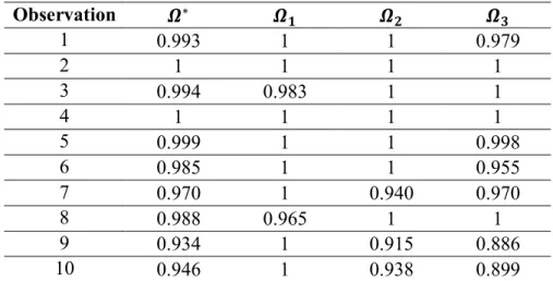
4.4 Results Validation ... 62
Chapter 5 Conclusions and Future Work ... 71
5.1 Conclusions ... 71
5.2 Future Work ... 71
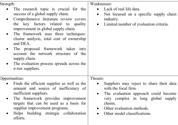
5.3 SWOT analysis ... 72
References ... 73
vii
List of Figures
Figure 1.1 Toyota vehicles recall in 2010 (Edwards, 2010, February 4) ... 2
Figure 2.1 Supply chain example (Regan, 2015) ... 5
Figure 2.2 Multi-tier supply chain ... 7
Figure 2.3 Hierarchical Structure ... 17
Figure 3.1 A sample dendrogram ... 36
Figure 3.2 Best cut method ... 37
Figure 4.1 Dendrogram with best cut ... 48
Figure 4.2 Example of 3-tier suppliers ... 50
Figure 4.3 Suppliers' efficiency scores ... 54
Figure 4.4 Efficiencies of the three suppliers ... 55
Figure 4.5 The supply chain of the Iranian beverage corporations’ case ... 63
viii
List of Tables
Table 2.1 Dickson supplier evaluation criteria ... 11
Table 2.2 Total cost of ownership literature review ... 13
Table 2.3 AHP Measurement Scale ... 18
Table 2.4 Summary of popular supplier evaluation techniques ... 26
Table 2.5 de Boer et al. (2001) supplier selection framework ... 28
Table 3.1 TCO costs' Categories ... 39
Table 4.1 Hypothetical upstream suppliers ... 45
Table 4.2 Normalized Data ... 46
Table 4.3 Weighted product types ... 47
Table 4.4 Cluster analysis final results ... 48
Table 4.5 Descriptive statistics ... 49
Table 4.6 Hypothetical data generated using Excel random routine ... 53
Table 4.7 Efficiency scores ... 54
Table 4.8 Input targets ... 56
Table 4.9 Efficiency scores without manufacturing cost... 58
Table 4.10 Efficiency scores without technology cost ... 58
Table 4.11 Efficiency scores without quality cost ... 59
Table 4.12 Efficiency scores without price ... 59
Table 4.13 Efficiency scores without logistics cost ... 60
Table 4.14 Efficiency scores without after sale cost ... 60
Table 4.15 Efficiency scores without social and environmental costs ... 61
ix
Table 4.17 The data of the Iranian beverage case study ... 69 Table 4.18 Calculation results of the Iranian beverage case study ... 69
1
Chapter 1
Introduction
With the complexity of today’s supply chains; firms have difficulty keeping track of all the activities happening in the supply chain. Less visibility and control of key processes have become the result of manufacturing, logistics and other roles such as outsourcing (Morehouse and Cardoso, 2011). As a result, the supply chain is now more vulnerable to frauds than before. Babies got poisoned by contaminated milk in China (Bradley, 2008) because one supplier decided to use melamine instead of protein nitrogen to gain some extra profit. In 2007, Canadian pet food manufacturing and retailer, Menu Food, had a massive recall of one popular pet food product because it caused sickness and death of animals as a result of high melamine level in some ingredients imported from Chinese suppliers (Chen et al., 2014). Moreover, Mattel recalled millions of toys in 2007 because the used paint contained high level of lead (Viswanadham and Samvedi, 2013).2
Figure 1.1 Toyota vehicles recall in 2010 (Edwards, 2010, February 4)
As a result, firms have strived to achieve successful supply chain collaboration. Collaboration can improve the traceability and visibility among the supply chain (Sarpong, 2014), which in turn improves the quality of the final product or service. Moreover, collaboration can deliver significant benefits to all parties such as excess inventory reduction, bullwhip avoidance, business synergy enhancement, flexibility and increase joint innovation (Cao and Zhang, 2011). Supply chain performance enhancement (Vereecke and Muylle, 2006) by leveraging the knowledge and resources of suppliers (Cao and Zhang, 2011) are some results of a successful collaboration.
Although product design, warehousing, and distributions centers can all be the subject of quality improvement programs; in this thesis we are focusing on purchasing as it contributes the most to the cost of quality. Both supplier evaluation and selection are essential for the success of the focal firm (Choi and Hartley, 1996; Singh, 2014). We argue that evaluation of the current suppliers is
3
the first step toward a successful collaboration relationship. Evaluation will reveal the weak areas of each supplier and recommend methods for improvement. Moreover, this evaluation will be the basis for supplier development program. We propose an approach based on Total Cost of Ownership (TCO) and Data Envelopment Analysis (DEA) due to their respective advantages. TCO looks beyond the quoted cost to cover additional true costs related to the entire purchasing cycle. In addition to the quoted price, it may include order placement costs, research costs, transportation costs, receiving costs, inspection costs, holding costs, and disposal costs (Bhutta and Huq, 2002). Consequently, TCO would help to understand the true costs associated with the quality of the purchased items.
DEA is a powerful non-parametric analysis technique that considers both quantitative and qualitative data. DEA does not require the decision maker to assign weights to each indicator but calculates weights from the given data. Additionally, DEA finds the efficient decision making units (suppliers) and computes the amount and source of inefficiency of inefficient suppliers (Cooper et al., 2007). It provides improvement targets for inefficient suppliers to become efficient. These targets values can be the basis of a new supplier improvement program.
1.1
Problem Definition
Supplier evaluation process is very critical to purchasing management. It is a complex multiple criteria decision making problem that requires careful selection of criteria (Omurca, 2013). Both qualitative and quantitative criteria should be used in evaluating the supplier performance. Additionally, it should speak the language of business, or money, to ensure acceptance among purchasing managers. It must also reflect the network structure of the supply chain. As a result, all the n-tier suppliers and the linkages between them should be evaluated for overall quality management in supply chains.
4
The aim of this thesis is to develop a multi-tier supplier quality evaluation framework for improving the quality of global supply chains. This involves:
1. Grouping of upstream suppliers using hierarchical cluster analysis 2. Evaluation of supplier quality at multiple tiers.
3. Identification of improvement targets for poorly performing suppliers and recommendations generation.
5
Chapter 2
Literature Review
2.1
Challenges for quality management in global supply chains
Mentzer et al. (2001) define supply chain as a set of firms that have direct upstream and downstream flows of products, services, finances, and information from a source to a customer. According to Bozarth and Handfield (2006), supply chain can be defined as a network of manufacturers and service providers that work together to transform and transport goods from the raw materials stage through the end user. Figure 2.1 illustrates the various stakeholders involved in a supply chain.
6
Supply chain can be classified into two main categories: product supply chain and service supply chain. Automobiles, electronics, fresh foods are some examples of product supply chain. Examples of service supply chain are healthcare, education, banking etc. The quality management practices may vary depending on the nature of supply chain. For example, fresh fruit supply chains have a long lead-time and a very high uncertainty level with regards to supply and demand. It requires an efficient management and the use of modern decision technology tools (Soto-Silva et al., 2015). Automobiles industry have very complex supply chains that start from extracting the basic raw materials until the delivery of final product. These supply chains requires innovative approaches to manage different supply chain activities (Vonderembse et al., 2006). In electronics supply chain, demand uncertainty and inventory control challenges are the main side effects due to the short life cycle of these products. Moreover, the complexity of these products requires a wide range of supply materials (Tse et al., 2016). For service supply chains, e.g. healthcare, the supply chain starts from supplying state of the art equipment and medicines from warehouses to clinics and hospitals. Management faces major challenges in managing these supply chains because of their great impacts on public health. It requires precise medical supply according to patient’s needs (Jahantigha and Malmir, 2015).
In today’s world it is not possible for a single organization to own its entire supply chain like the Ford Company in the first half of the 20th century (Gelderman, 1989). To stay competitive in
global market; organizations have to outsource many critical business processes and value chain activities to suppliers thousands of miles away to reduce cost or increase responsiveness (Nieminen and Takala, 2006). Therefore, the supply chain has become more and more complex. Especially when the direct supplier (first tier) outsources part of its business to another supplier
7
(second tier). In this case we have multi-tier suppliers and a multi-tier supply chain. Figure 2.2 presents the diagram of a multi-tier supply chain.
Figure 2.2 Multi-tier supply chain
With globalization, organizations face several challenges in managing supply chain quality (Jain and Benyoucef, 2008; Kuei et al., 2011; Morehouse and Cardoso, 2011; Tse and Tan, 2011; Klassen and Vereecke, 2012; Tachizawa and Wong, 2014). To name a few are:
Less visibility and control of key processes
8 Protecting the environment
Considering the environment in order to survive in today’s environmentally conscious market.
Social issues
Labour practices by global suppliers in developing countries, which includes worker safety, working conditions, workers’ rights and child’s labour.
Inventory reduction
Applying JIT philosophy can lead to significant cost-savings, however, the supply chain may become more vulnerable as they have very little inventory to buffer any interruptions in supply.
Adopting advanced technologies
To facilitate effective decision making; firms should identify technology applications that participate effectively in the global progress. Examples of such technology are enterprise resource planning (ERP), customer relationship management (CRM), and product lifecycle management (PLM).
Therefore, firms are striving to achieve successful supply chain collaboration to limit some of these impacts. Collaboration can improve the traceability and visibility among the supply chain members (Sarpong, 2014), which in turn improves the quality of the final product or service.
2.2
Collaboration for improving supply chain quality
Anthony (2000) stated that supply chain collaboration occurs “when two or more companies share the responsibility of exchanging common planning, management, execution, and performance measurement information”. Furthermore, he suggested “Collaborative relationships
9
transform how information is shared between companies and drive change to the underlying business processes”.
In today’s business environment; collaboration is more important than ever as technologies are rapidly changing, competition is growing, outsourcing is increasing, and the growth of very specialised companies is taking place (Sarpong, 2014). Several authors have discussed the benefits of successful collaboration. We mentioned some of these benefits in the previous chapter. Other benefits include more sales volume from downstream buyers, lower operational costs, word-of-mouth referrals, and new product and process innovations resulting from a working relationship between trusting partners (Sarpong, 2014). Additionally, collaboration improves and assists the environment and social aspects of sustainability (MacCarthy and Jayarathne 2012).
Many firms have started to realize that it is not enough to collaborate with the first-tier suppliers only. To achieve the full potential benefits of collaboration; firms should collaborate with lower tier suppliers as well. For example, Puma’s sustainability report covers up to the fourth tier of suppliers, and Nike is auditing hundreds of second-tier apparel suppliers (Lee et al., 2012). IKEA is working with its suppliers to comply with the code of conduct (Andersen and Skjoett-Larsen, 2009). Similarly, Hewlett-Packard and Migros manage sub-suppliers to ensure they fulfill the requirements of corporate sustainability standards (Grimm et al., 2014).
The first step in collaboration is partner selection which starts with supplier evaluation in buyer-supplier partnerships. In the following section we will explore different approaches for buyer-supplier evaluation and reveal their weaknesses and strengths.
10
2.3
Evaluating supplier quality
Supplier evaluation is a multi-criteria decision making problem that involves several qualitative and quantitative factors. Several studies have been conducted to develop decision-making models that can address this problem effectively (Zeydan et al., 2011). Ghodsypour and O’Brien (1998) classify supplier evaluation models into two groups: single objective models and multiple objective models. Single objective models use one criterion, such as the cost, as an objective function and other criteria as constraints. This approach has two weaknesses: it weights all constraints equally which rarely happens in reality, and it faces significant difficulties when considering qualitative factors. Moreover, it is very risky to rely on a single criterion when evaluating a supplier. Therefore, using a multi-criteria approach is preferable over the single criterion approach (Zeydan et al., 2011).
One of the earliest contributions to supplier evaluation and selection criteria was of Dickson (1966). In his study he identified 23 criteria for supplier evaluation. Furthermore, he found that quality, delivery and performance history are the most important criteria (see Table 2.1). Erdem and Gocen (2012) list 60 criteria for supplier evaluation among which price, quality, availability and delivery are the most significant ones. These results confirm the multi-criteria nature of supplier evaluation problem.
11
Evaluation Criteria Rank
Quality 1
Delivery 2
Performance History 3
Warranties and claim policies 4
Production facilities and capacity 5
Price 6
Technical capability 7
Financial position 8
Procedural compliance 9
Communication system 10
Reputation and position in industry 11
Desire for business 12
Management and organization 13
Operating controls 14
Repair service 15
Attitude 16
Impression 17
Packaging ability 18
Labor relations record 19
Geographical location 20
Amount of past business 21
Training aids 22
Reciprocal arrangements 23
Table 2.1 Dickson supplier evaluation criteria
According to Ho et al. (2010) and Erdem and Gocen (2012), supplier evaluation and selection approaches can be classified into:
Linear weighting models such as Analytic hierarchy process, interpretative structure modeling, fuzzy set theory, and total cost of ownership.
Mathematical programming models such as data envelopment analysis, linear programming, mix integer programming, and goal programming.
Artificial intelligence models and Statistical/probabilistic models such as case based reasoning, genetic algorithm, neural network, and expert systems.
Supplier evaluation should be extended beyond the first-tier suppliers to cover all suppliers across the supply chain. Many researches consider this as one way to manage the supply chain (Rao,
12
2002; Zhu and Sarkis, 2004;Andersen and Skjoett-Larsen, 2009; Mueller et al., 2009; Zhu et al., 2012). Ho et al. (2010) and Noshad and Awasthi (2015) reviewed several published articles on multi-criteria decision making approaches for supplier evaluation and selection. DEA was the most popular individual approach per Ho et al. (2010) while AHP and DEA based approaches were the most popular per Noshad and Awasthi (2015). In the following section we will examine popular approaches found in literature. Additionally, a summary for these approaches is presented in table 2.4.
2.3.1 Total Cost of Ownership (TCO)
An IT research and advisory company called Gartner was the original developer of the total cost of ownership (TCO) concept in 1987. They used it to compute the total costs of owning and managing IT infrastructure in a company (Bermen et al., 2007). Later, the concept has been used to calculate total cost of purchased goods in general (Ellram, 1993). TCO is a purchasing tool and a philosophy which is aimed at understanding the real cost of buying a particular good or service from a supplier (Ellram, 1995). It is a complex approach that requires the firm to determine the associated costs and find ways to quantify non-monetary costs if they want to better understand and manage their costs. It may include in addition to the quoted price, order placement costs, research costs, transportation costs, receiving costs, inspection costs, holding costs, and disposal costs (Bhutta and Huq, 2002).
Although there are other selection and evaluation approaches closely related to TCO, such as life-cycle costing, zero-base pricing, cost-based supplier evaluation, and cost ratio method, none of them received significant, widespread support in literature or in practice (Ellram, 1995). Complexity, situation-specific application, over-reliance on some factors and inadequate
13
consideration of others are some of the factors that could be the reasons behind the lack of support (Bhutta and Huq, 2002).
Author, Year Incentive to Use TCO TCO Cost Categories
Bhutta and
Huq (2002) Supplier Selection Manufacturing Quality Technology After sales services Degraeve and
Roodhooft (1999)
Supplier Selection Three hierarchic levels: Supplier level activities Ordering level activities Unit level activities Degraeve et
al. (2005) Evaluating organization’s strategic procurement options
Purchasing managers performances evaluation Understanding the costs of purchasing
activities
Cost matrix of supplier, product, order, unit (cash, non cash) versus acquisition, reception, possession, utilization, elimination Dogan and
Aydin (2011) Supplier Selection Product design cost Downtime cost Logistics cost Operation cost Quality related cost Administrative cost Transaction cost Ellram (1993) Supplier performance evaluation
Decision making Supplier selection
Understanding the costs of purchasing activities
Pre-Transaction costs Transaction costs Post-Transaction costs Hurkens et al.
(2006) Negotiating prices Identify and prioritize improvement actions Understand the consequences of changing
volume allocation among suppliers.
Dealer buy
Quality confirmation Quality check Adverse buy
Warehousing (Handling, Inventory holding, Storing) Supplier returns
Supplier monitoring Cash flow
Maltz and
Ellram (1997) Including non-monetary factors into make/buy decisions
Management Quality Delivery Service Communications Price
14
On the other hand, there has been more focus on TCO among the published articles. Table 2.2 highlights some of these articles along with the incentives of using TCO and the cost categories suggested by different researchers. It can be seen that many researches have considered supplier selection as the main reason for choosing TCO while others considered supplier evaluation as the main motive. But the common reason is to reveal the true cost of purchasing activities (Ellram, 1993). Only (Maltz and Ellram, 1997) considered it from another perspective by incorporating TCO into the make/buy decision.
2.3.1.1 Barriers to TCO
Despite these efforts, TCO is still a complex approach and many organizations face a lot of difficulties and barriers when trying to implement it. Ellram (1995) considered lack of an accounting and costing system as a major challenge. Many organizations use activity based costing as a way to overcome this barrier (Ellram, 1993; Ellram, 1995; Sohal and Chung, 1998). Culture change is another barrier, a change from price orientation towards understanding total cost. That’s why TCO is considered more a philosophy than a tool (Ellram, 1995). Furthermore, there is no standard model for TCO analysis. Using TCO models may vary inside the organization according to the importance of the purchase (Ellram, 1995; Ferrin and Plank, 2002).
2.3.1.2 Benefits of TCO
TCO delivers many benefits to organizations. Cost transparency is pointed as the basic advantage of applying a TCO approach (Bremen et al., 2007). Other benefits considered by Ellram (1995) are improving the supplier evaluation and selection process, defining the supplier performance expectations for the organization and the supplier, help prioritize areas in which supplier performance would be most beneficial (such as supplier continuous improvement), creating
15
major cost saving opportunities, improving firm’s understanding of supplier performance and cost structure, and using cost information as a basis for supplier negotiations. Only Bhutta and Huq (2002) pointed out that TCO helps in building strategic collaboration efforts.
2.3.1.3 TCO Cost Categories
Table 2.2 illustrates that authors categorized cost according to the functional departments in an organization. Maltz and Ellram (1997) used the categories as management, quality, delivery, service, communications, and price. Ellram (1993) suggested a more general approach based on the order of occurrence: pre-transaction costs, transaction costs, post-transaction costs. Pre-transaction costs involve all costs related to activities that occur prior to order placement such as identifying requirements, searching for a supplier, negotiation, and supplier evaluation. Transaction costs occur at the time of purchasing and receiving the ordered item. Price, delivery charges, and inspection are some examples of transaction costs. Post-transaction costs occur after closing the order. In other words, post- transaction costs include all activities that happen after the organization owns the ordered item such as maintenance costs and quality failures costs (Ellram, 1993).
Hurkens et al. (2006) conducted a study on a service sector organization (a vehicle glass repair and replacement company) to show how TCO information can influence strategic decision regarding allocation of volumes. They used the cost categories as buying from dealer, quality confirmation, quality check, adverse buy, supplier returns, supplier monitoring, and cash flow. Bhutta and Huq (2002) categorized production into manufacturing, quality, technology, and after sales services costs to compare between total cost of ownership and analytic hierarchy process approaches. Manufacturing costs include raw material, labor, and machine depreciation. Quality costs are related to activities performed to monitor and control quality such as inspection, cost of
16
rework, and scrap. Designing and engineering costs are some examples of technology costs. Finally after sales costs are related to after sales activities such as warranty and customer claims (Bhutta and Huq, 2002; Garfamy, 2006).
Degraeve and Roodhooft (1999) developed a decision-making model to minimize TCO when selecting a supplier. The model is based on three hierarchical levels. The first level is the supplier’s activities that are performed when a specific supplier is used. For example, inspection and quality audit. On the next level we have ordering level activities. Activities on this level should be performed each time an order is assigned to a supplier. Unit level activities are at the last level and performed for a unit in a specific order. For example, production downtown cost related to a defective item purchased from a supplier.
Degraeve et al. (2005) presenting a matrix model consisting of supplier level, product level, order level, and unit level activities and their associated life cycle costs. Furthermore, Dogan and Aydin (2011) proposed a model that combines total cost of ownership and Bayesian networks to efficiently select a supplier using product design cost, downtime cost, logistics cost, operation cost, quality related cost, administrative cost, and transaction cost as the cost categories.
Researchers have presented different costs categories to serve different purposes as can be seen from the previous section but no study so far, according to our knowledge, suggested cost categories from collaboration perspective. This thesis is trying to fulfill this gap by incorporating collaboration into our selection of the cost categories.
2.3.2 Analytic Hierarchy Process (AHP)
Saaty first developed the Analytic Hierarchy Process (AHP) method in 1980. AHP provides a multiple criteria framework for situations involving intuitive, rational, quantitative, and
17
qualitative aspects. It provides a mathematical model to assign weights to multiple alternatives using a scheme of pairwise comparison (Singh, 2014). AHP allows complex problems to be represented in a hierarchical form that consists of at least three levels, the goal, the criteria, and the alternatives (Bhutta and Huq, 2002). Figure 2.3 shows an example of the hierarchal form of AHP in the supplier evaluation context.
Figure 2.3 Hierarchical Structure
Managerial experience then will drive the computations by assigning weights to each criterion. Thus, quantifying the managerial experience is required at this stage. According to Bhutta and Huq (2002), the scale presented in Table 2.3 is the most common scale used for this analysis. Next step is to construct a matrix that compares each criterion with other using this measurement scale.
18
Preference Numerical Scale
Extremely preferred 9
Very strongly to extremely
preferred 8
Very strongly preferred 7
Strongly to very strongly
preferred 6
Strongly preferred 5
Moderately to strongly preferred 4
Moderately preferred 3
Equally to moderately to
strongly preferred 2
Equally preferred 1
Table 2.3 AHP Measurement Scale
Once the matrix is ready we can start the calculation process as follows: 1) Compute the sum of each column.
2) Divide each cell by the column total. 3) Calculate row averages.
Similarly, we develop the suppliers’ matrix by assigning a score to each supplier with respect to the criteria under consideration. Then, the above steps are followed to calculate the weight of each supplier. Finally, the scores of each supplier are calculated by multiplying the founded scores in the criteria matrix with the weights in the suppliers’ matrix, which give us the final scores of each supplier.
Many researchers have used AHP for supplier selection and evaluation (Akarte et al., 2001; Muralidharan et al., 2002;Chan, 2003; Liu and Hai, 2005; Hou and Su, 2007; Bruno et al., 2012; Deng et al., 2014) due to the flexibility, simplicity, and the capability of this approach to incorporate both quantitative and qualitative criteria. On the other hand, AHP has the
19
disadvantage that the number of pairwise comparisons may become very large when having many alternatives and criteria (𝑛(𝑛 − 1)/2). Additionally, another disadvantage is the artificial limitation of the 9-point scale. For instance, if alternative X is 5 times more important than alternative Y, which is 5 times more important than alternative Z. In this case, it is not possible for AHP to handle the fact that alternative X is 25 times more important alternative Z (Macharis et al., 2004).
2.3.3 Goal Programming (GP)
Charnes and Cooper first presented this technique in 1961. Later, Lee and Ignizio improved it in 1972 and 1976 respectively. Goal programming (GP) is a multi-objective decision making technique (Bal et al., 2006). GP involves a set of goals that may often contradict each other. Therefore, it is not possible to satisfy all goals at the same time as achieving one goal may cause another goal to deviate from its own target. Thus, the purpose of GP is to minimize the deviation between achievement of goals and their aspiration levels (Liao and Kao, 2010).
To construct a GP model, we use the following steps (Ignizio, 1976): i. Define the decision variables.
ii. Determine the goal and system constraints.
iii. Decide the preemptive priority factors and the relative weights. iv. Define the nonnegative requirement.
The mathematical formulation for GP can be as following (Romero, 2004): Min ∑q𝑖=1| 𝑓j(𝑋) − 𝑏𝑖|
subject to 𝑋 ∈ 𝐹
20
𝐹 is a feasible set
𝑋 is an element of 𝐹
𝑓j(𝑋) is a linear function of 𝑖𝑡ℎ goal.
𝑏i is the aspiration level of the 𝑖𝑡ℎgoal.
𝑞 is the total number of goals
GP is useful in the cases of multiple goals that are conflicting and not all achievable. Subsequently, goal programming allows ranking of goals so that the lower priority goals are considered only when higher priority goals are fully satisfied. Also GP is useful when a satisfactory solution is required rather than an optimized solution (Hughes and Grawoig, 1973). As a result, various studies used GP for supplier selection and evaluation either as an individual approach or combined with other approach such as AHP. For instance, Karpak et al. (2001) and Osman and Demirli (2010) developed GP model to evaluate suppliers and allocate orders. Çebi and Bayraktar (2003) applied an integrated AHP-GP approach for supplier selection. Weights of suppliers were evaluated using AHP. Then the GP model uses these weights as an input for finding the best supplier. Wang et al. (2004), Perçin (2006), Kull and Talluri (2008), Mendoza et al. (2008) and Erdem and Gocen (2012) presented different AHP-GP approaches for supplier selection and evaluation.
GP has some problems. One major problem arises from the requirement of setting the goal achieving order, i.e., the weights of each goal. If the model did not produce an acceptable solution then the purchasing managers may alter the priority structure until an acceptable solution is generated. This may be costly and time consuming (Karpak et al., 2001). Furthermore, the goal achievement nature of GP may not be appropriate for supplier evaluation for the purpose of
21
collaboration. As stated before, GP will not achieve all goals at the same time and the generated solution is satisfactory rather than an optimum one.
2.3.4 Data Envelopment Analysis (DEA)
2.3.4.1 Basic Model
DEA is a popular technique for supplier evaluation and selection (Braglia and Petroni, 2000; Liu
et al., 2000; Forker and Mendez, 2001; Narasimhan et al., 2001; Talluri and Baker, 2002; Talluri and Sarkis, 2002; Talluri and Narasimhan, 2004; Garfamy, 2006, Ross et al., 2006; Saen, 2006; Seydel, 2006).
DEA was originally developed by (Charnes et al., 1978) to evaluate non-profit and public sector organizations. It was known as the Charnes, Cooper and Rhoades (CCR) model. Since then DEA has become one of the most effective techniques to measure the performance of organizations such as business firms, government departments, hospitals etc. It does not require the decision maker to define weights for each indicator. It simply calculates the weights from the given data. Moreover, DEA is capable of distinguishing the benchmark entities based on the efficiency score and finding the amount and source of inefficiency of inefficient entities (Cooper et al., 2007). The objective of DEA is to find the efficiency score of all units under evaluation. These units are called decision-making units or (DMUs). DMU is defined as an entity that consumes inputs to produce outputs and whose performance is to be evaluated (Cooper et al., 2007). DMUs can be the members of a supply chain, firms or simply departments of a single organization.
The first step in evaluating the performance of a DMU is finding a virtual DMU that will be the most efficient unit (called efficient frontier). Then DEA compares all DMUs to the efficient frontier to find their efficiency scores. The efficiency score is defined as weighted sum of outputs
22
divided by weighted sum of inputs. This does not mean we need to assign weights as DEA calculates weights automatically based on the given inputs and outputs. Cooper et al. (2007) set the following rules for selecting the inputs and outputs:
All inputs and outputs should have numerical data which is assumed to be equal or greater than zero.
The selection of inputs, outputs and DMUs should be relevant to the study. Efficiency scores should reflect the following principles:
i. Smaller input amounts are preferable. ii. Larger output amounts are preferable.
The measurement units across the different inputs and outputs should not be the same. Suppose we have 𝑛 different DMUs and each one has 𝑚 input items and 𝑠 output items.
Efficiency = Sum of weighted outputs Sum of weighted inputs
which can be reformulated per CCR-DEA (Cooper et al., 2007) into the following linear program: Min𝜃𝑝 ∑ 𝑥𝑛𝑗 𝑖𝑗𝜆𝑗≤ 𝜃𝑝𝑋𝑖𝑝 for all 𝑖 = 1, … . , 𝑚 subject to ∑ 𝑦𝑛 𝑟𝑗𝜆𝑗 ≥ 𝑦𝑟𝑝 𝑗 for all 𝑟 = 1, … . , 𝑠 ∑ 𝜆𝑛 𝑗 = 1 𝑗 where:
𝜃𝑝 is the efficiency score of DMUp ( the DMU under evaluation )
23
𝑦𝑟𝑝 is the produced amount of output 𝑟 by DMUp
𝜆𝑗 is the computed weights associated with DMUj determining whether it is a benchmark for
DMUp
𝑥𝑖𝑗 is the consumed amount of input 𝑖 by DMUj
𝑦𝑟𝑗 is the produced amount of output 𝑟 by DMUj
The above equations simply mean that the computed virtual DMU should satisfy two conditions: (i) consume the same or less input amount than DMUp. (ii) Produce the same or more output than
DMUp.
Moreover, we should note the following: i. DMUp is efficient when 𝜃𝑝 = 1. ii. DMUp is inefficient when 𝜃𝑝 < 1. iii. Efficiency cannot be greater than 1.
2.3.4.2 Network DEA
The major drawback of traditional DEA is that it treats DMUs as a “black box” by considering only the initial inputs and the final outputs and omits the actual activities happening inside (Lewis and Sexton, 2004; Kao, 2009; Zhu, 2009; Azbari et al., 2014; Yang et al., 2014). For example, traditional DEA can be used for selecting an efficient supplier among proposed suppliers for a new product but it cannot be used to evaluate the current upstream suppliers, as it will ignore the sub-suppliers and current linkages between them. Therefore, network DEA is preferable in these cases for its advantages over the traditional DEA. Specially, its ability to detect efficiencies missed by the traditional DEA. Network DEA considers the intermediate linkages as the outputs of the previous stages and the inputs to the next stage.
24
Many approaches for network DEA have been presented over the years. Aoki et al. (2010) developed a network DEA model based on the RAM model presented by Cooper et al. (1999) to optimize the supply chain. Mirhedayatian et al. (2014) proposed a network DEA model to assess green supply chain management in the existence of dual-role factors, undesirable outputs, and fuzzy data. Tajbakhsh and Hassini (2014) developed a multi-stage DEA capable of evaluating the sustainability of the supply chain members. Chen and Yan (2011) created three network DEA models to evaluate the performance of supply chains under the concept of centralized, decentralized, and mixed organizational mechanisms.
Despite its many benefits, DEA has some drawbacks. First, the decision-maker may be confused when defining the input and output criteria. Second drawback comes from the subjective assignment of qualitative criteria. Finally, DEA finds the efficient supplier who generates more output while using less input. Therefore, can an efficient supplier be considered an effective one? (Ho et al., 2010).
This thesis is using the network DEA model presented by Zhu (2009) which embodies the structure of the supply chain to define and evaluate efficiency of the supply chain and its individual members. Moreover, the model yields a list of optimal values for all members that establish an efficient supply chain.
25
Technique Description Benefits Drawbacks Supplier evaluation in
literature
TCO A purchasing tool which is aimed at understanding the real cost associated with the entire purchasing cycle
Cost transparency Improves supplier
evaluation and selection process
Defines the supplier performance expectations Helps prioritising supplier
performance areas
Cost savings opportunities Better understanding of
supplier performance and cost structure
Can be the basis for supplier negotiations
Helps building strategic collaboration efforts.
Complex approach as it may require methods to
quantifying non-monetary costs
Lack of an accounting and costing system
Requires culture change No standard model
Ellram (1993);Degraeve and Roodhooft (1999);Dogan and Aydin (2011);Bhutta and Huq (2002)
AHP A mathematical model that allows complex problems to be represented in a hierarchal form.
Flexibility Simplicity
Can incorporate quantitative and qualitative criteria
Very complex pairwise comparisons in case of many alternatives and criteria.
Artificial limitation of the 9-point scale.
Akarte et al. (2001); Muralidharan et al. (2002); Chan (2003); Liu and Hai (2005); Hou and Su (2007); Bruno et al. (2012); Deng et al. (2014)
GP A multi-objective decision making technique that involves a set of goals that may
contradict with each other.
Helps when we have multiple goals that are conflicted and not all achievable.
Allows ranking of goals so that the lower priority goals are considered only when higher priority goals are fully satisfied
Can be used when satisfied solution is required rather
Can be costly and time consuming
The generated solution will be a satisfactory solution rather than an optimum one
Karpak et al. (2001); Çebi and Bayraktar (2003);Wang et al. (2004); Perçin (2006); Kull and Talluri (2008); Mendoza et al. (2008); Osman and Demirli (2010); Erdem and Gocen (2012)
26 than an optimized solution
Technique Description Benefits Drawbacks Supplier evaluation in
literature
DEA A linear programming based technique to measure the
efficiency of a set of entities that have multiple inputs and
outputs.
Non-parametric analysis technique
Considers both quantitative and qualitative data
Finds the efficient supplier as well as the amount and source of inefficiency of inefficient suppliers Provides improvement
targets
May draw confusion when defining the input and output criteria
Subjective assignment of qualitative criteria Can mislead the purchase
manager, as efficient supplier may not be an effective one.
Braglia and Petroni (2000); Liu et al. (2000); Forker and Mendez (2001); Narasimhan et al. (2001); Talluri and Baker (2002); Talluri and Sarkis (2002); Talluri and Narasimhan (2004); Garfamy (2006); Ross et al. (2006); Saen (2006); Seydel (2006)
27
2.4
Supplier Quality Evaluation Framework
de Boer et al. (2001) developed a decision making framework for supplier selection that expands the purchasing model of Faris et al. (1967) and the model of Kraljic (1983) to include more situations that are not usually found in literature. They differentiate between three types of procurement situations: first time buy, modified rebuy, and straight rebuy of routine and strategic items. Additionally, they propose four phases of the supplier selection process: problem formulation, formulation of criteria, qualification, and supplier selection. Their framework is presented in table 2.5.
First time buy situation usually consists of a brand new product or service with unknown suppliers. In this phase, the level of uncertainty is the highest and no previous historical data about the suppliers is available. As a result, this is the most complex procurement situation and group decision-making is required to solve it.
Modified rebuy is related to buying a new product or service from a known supplier or buying a modified or existing product from a new supplier. The uncertainty level in this case is moderate. On the other hand, in straight rebuy situation we have enough information about the required product or service. Furthermore, an agreement already exists with a known supplier and it is just a matter of placing an order.
28
First Time Buy Modified Rebuy
(Leverage Items)
Straight Rebuy (Routine Items)
Straight Rebuy (Strategic Items) Problem Definition Whether to use a supplier or
not
Either to use more, less or other suppliers
Do we need to replace the current supplier?
How to deal with the current supplier?
Formulation of
Criteria
Various importance levels Unrepeatable decision No previously defined
criteria or suppliers historical data available
Moderate to high importance
Repeatable decision Previously defined
criteria and suppliers historical data available
Low to moderate importance
Repeatable decision Previously defined
criteria and suppliers historical data available
High importance Repeatable evaluation Previously defined
criteria and suppliers historical data available
Qualification Various importance levels Small initial set of
suppliers
Sorting rather than ranking
No historical data available
Large number of initial suppliers
Sorting and ranking Historical data available
Large number of initial suppliers
Sorting rather than ranking
Historical data available
Very small number of suppliers
Sorting rather than ranking
Historical data available
Choice Small initial set of suppliers
Ranking rather than sorting
Several criteria A lot of interaction No historical data
available
Various importance levels One time used
Small to moderate
number of initial suppliers Ranking rather than
sorting
How to allocate volume? Less criteria
Fewer interaction Historical data available Model can be used again
Small to moderate
number of initial suppliers Ranking rather than
sorting Less criteria Fewer interaction Historical data available Model can be used again Single sourcing rather
than multiple sourcing
Very small number of suppliers (usually one) Historical data available It is evaluation rather than
selection Sole sourcing
29
It can be noticed from table 2.5, that although de Boer et al. (2001) presented different important levels for the first buy situations but steps of the supplier selection process are the same regardless of the importance. In the rebuy situations, selection steps may vary. In the following paragraphs we will show how de Boer et al. (2001) linked these variations to Kraljic (1983) model.
Kraljic (1983) classified the purchase items into leverage, strategic, bottleneck, and routine. In the case of routine item, de Boer et al., (2001) indicated that it is not worthy for an organization to frequently search for new suppliers that could supply the item because of its low value. Therefore, similar routine items are usually purchased from one or two suppliers. As per de Boer
et al. (2001) any modification related to the specifications of the purchased items are dealt by the current supplier. An evaluation of the supplier is carried out periodically and a new supplier is selected if needed.
Similarly, bottleneck and strategic items have fixed suppliers. The current supplier deals with any changes to the specifications of these items. The reason behind this is different from that of the routine items. These items involve high supply risk because of their unique specifications or the rare material. Therefore, the decision models are only for evaluation and monitoring these suppliers.
On the other hand, modified rebuy situations are usually related to leverage items. In this case, there are many suppliers to select from. A frequent selection of suppliers occurs more often because of high value of these items. An agreed vendor list is the outcome of the first three steps (Problem definition, formulation of criteria and prequalification) and the final supplier is selected from this list (de Boer et al., 2001).
30
In the section below, we will list the different methods found in literature for different phases of supplier selection process.
2.4.1 Problem definition and formulation of criteria
For the problem definition phase, there are not many works on supplier selection. de Boer et al.
(2001) found two methods that can be used for formulation of criteria. The first technique is called Interpretive Structural Modelling (ISM). The second method is an expert system that covers different phases in the selection process including the supplier selection criteria. This system is based on literature review and knowledge of a senior purchasing manager.
2.4.2 Pre-qualification
de Boer et al. (2001) defined pre-qualification as the process of selecting an acceptable set of suppliers from the whole set. The methods commonly used in this phase are categorical methods, data envelopment analysis, cluster analysis and case based reasoning systems.
In categorical methods, the supplier is evaluated based on both the buyer’s experience and historical data. The supplier is evaluated as positive, neutral or negative. The buyer later gives an overall rating and the suppliers are classified into these three categories.
de Boer et al. (2001) suggested DEA and cluster analysis for categorizing suppliers prior to the final selection. Case based reasoning can also be used. It is a software system based on artificial intelligence that aids decision makers with helpful information and experiences from past decisions.
31 2.4.3 Final choice phase
In this phase, linear weighting, total cost of ownership, mathematical programming, statistical and artificial intelligence based models are often used for selecting the appropriate suppliers (de Boer et al., 2001).
In linear weighting models, each criterion is given a weight. Then the weights are multiplied by the criteria ratings and summed. AHP is an example of this method.
Total cost of ownership is a tool and philosophy to achieve a better understanding of the real cost of buying a particular good or service from a supplier (Ellram, 1995). Mathematical programming models aid the decision maker in formulating the purchasing problem into an objective mathematical formula that should be maximized or minimized by altering the values of its variables (de Boer et al., 2001).
Statistical models deal with “stochastic uncertainty” related to supplier selection.
Finally, artificial intelligence based models are learning based software systems that can be consulted for selecting an appropriate supplier.
2.4.4 The Proposed Framework
de Boer et al. (2001) addressed supplier evaluation mainly at one level whereas in this thesis we propose a framework for multi-tier supplier evaluation. Therefore, we are dealing with a different problem as shown below:
Problem definition
Evaluate the current n-tier suppliers to study the possibility of collaboration. Formulation of criteria
The historical data is available as we are evaluating existing suppliers. Both qualitative and quantitative criteria are used in evaluating the supplier performance.
32 Qualification
Cluster analysis is used to classify suppliers into groups with similar characteristics. This is an essential step when there are a large number of suppliers whose evaluation can be costly and time consuming.
Final choice
This phase consists of two steps. First, we find the true cost associated to each supplier using TCO. In the second step, we use the TCO results as input to the DEA model to find the efficient suppliers. TCO and DEA help identify the weak points in supplier performances and suggest improvement targets. These improvement targets cannot be identified if we use another model than DEA in this phase.
33
Chapter 3
Solution Approach
Our solution approach involves three main steps:1. Grouping of upstream suppliers using hierarchical cluster analysis 2. Multi-tier supplier quality evaluation using TCO and DEA
3. Identifying targets for improving poor quality suppliers performance
3.1
Grouping of upstream suppliers using hierarchical cluster analysis
The first step involves classifying suppliers into groups on the basis of similar characteristics. This is an essential step when there are a large number of suppliers that make the evaluation process costly and time consuming. In this step, we will classify only the first-tier suppliers as the lower-tier suppliers will be grouped automatically based on their first-tier suppliers. We base our classification on the following criteria. These criteria were identified based on our previous experience with supply chain projects.
Cost of Quality
It is the cost related with avoiding poor quality or cost that is encountered as a result of poor quality. It can be categorized into prevention costs, appraisal costs, internal costs, and external failure costs (Evan and Lindsay, 2005).
Risk
Supply risk is defined as “the probability of an incident associated with inbound supply from individual supplier failures or the supply market occurring, in which its outcomes result in the
34
inability of the purchasing firm to meet customer demand or cause threats to customer life and safety” (Zsidisin, 2003).
Location
It is a numerical value to represent the supplier geographical location (country name). Product type
A numerical value to represent the type of product purchased from the supplier. For instance, raw material, spare parts, and packaging materials.
Organization profile (size)
It is the number of employees in supplier’s firm. Cost sustainability
Energy cost, water cost, social policies, fines and penalties.
3.1.1 Hierarchical Cluster Analysis
Hierarchical cluster analysis can be classified into: agglomerative approaches and divisive approaches. Agglomerative approach is a bottom-up approach where initially each value is a cluster in its own. Then each pair of clusters is merged together until only one cluster is left. On the other hand, divisive approach considers the whole dataset as one cluster at the beginning, and then splits them into further clusters (Al Salem, 2012).
In order to use these approaches, first distance measure needs to be chosen. Al Salem (2012) listed the following measures to find how two objects are similar or dissimilar:
1. Euclidean distance: It is a popularly used measure. Euclidean distance uses the formula
𝑑𝑖𝑗 = √∑k=1p (𝑥𝑖𝑘− 𝑥𝑗𝑘)2 to compute the distance between two objects 𝑥𝑖𝑘 and 𝑥𝑗𝑘 for
35
2. Manhattan distance: It calculates total absolute distance between two objects under the
𝑘𝑡ℎ variable value of the p-dimension using the formula, 𝑑
𝑖𝑗 = ∑pk=1|𝑥𝑖𝑘− 𝑥𝑗𝑘|. 3. Minkowski distance: The previous two measures are a special case of this one.
𝑑𝑖𝑗 = (∑pk=1|𝑥𝑖𝑘− 𝑥𝑗𝑘|𝑟)1/𝑟 𝑟 ≥ 1
Next step is to link the objects to clusters using one of the below linkage methods as per Al Salem (2012):
1. Single linkage distance: The linkage is determined based on the minimum distance between two objects.
2. Complete linkage: The linkage is determined based on the maximum distance between two objects.
3. Average linkage: The linkage is determined based on the average distance between elements of one cluster and the other clusters.
The linkage of objects to clusters will construct a tree diagram called dendrogram. A dendrogram shows how the elements of each cluster are connected and the distance at which clusters are joined. Figure 3.1 illustrates a sample dendrogram.
36
Figure 3.1 A sample dendrogram
In this thesis we are using hierarchical cluster analysis as it is a straightforward clustering technique. Moreover, this technique does not require the number of clusters to be known at the beginning. Once the dendrogram is constructed; the number of clusters can be retrieved from the diagram. We are using the best-cut method to find the number of clusters. Best-cut method is the largest distance width of range between two connected distances. For example in figure 3.2, the best cut lies between distance 19 and 12. This is because the width of range 𝑑𝑖𝑗 between distance 19 and 12 is equal 7 which is larger than between 12 and 8. Therefore, we have 3 clusters. Cluster 1 contains supplier 5, 6, 7, 3 and 4. Cluster 2 has supplier 1 and 2. Finally the remaining suppliers are in cluster 3.
37
Figure 3.2 Best cut method Thus, our grouping approach will be as follows:
1. Since our data variables are in different units, normalization is required. We will be using
the formula 𝑧 = (𝑥−𝑥̅)𝑠 where 𝑥 is the data value, 𝑥̅ is the mean, and 𝑠 is the standard
deviation.
2. Assigning weights to product type values to ensure that suppliers with the same product type stay together.
3. Applying hierarchical clustering using Euclidean distance measures and the complete linkage method.
38
3.2
Multi-tier supplier quality evaluation using TCO and DEA
Our evaluation framework is based on Total Cost of Ownership (TCO) and Data Envelopment Analysis (DEA). The first step involves finding the true cost associated to each supplier using TCO. We will go beyond the quoted price and try to figure out how much it will cost us if we continue dealing with the current suppliers. Furthermore, we will not just evaluate the first tier (direct) suppliers but all the n-tier suppliers. This is important if we are aiming towards a successful collaboration.
We will expand the model presented by Garfamy (2006) to include categories related to global supply chain collaboration. Our approach evaluates the whole upstream suppliers whereas Garfamy (2006) approach could be useful to select the best supplier among the suppliers supplying a given part. Therefore, to evaluate our networked suppliers we will need different DEA than the one Garfamy (2006) has used. We will use the Network DEA model presented by Zhu (2009) as stated in the previous chapter.
39
TCO Categories TCO Sub Categories Author Global
Context Measurement Method Product Vs.
Service
Input/ Output Manufacturing
Costs
Raw Material Bhutta and Huq (2002) Yes Quantitative costs P I
Labour Yes Quantitative costs P I
Machine depreciation Yes Quantitative costs P I
Quality Costs Quality Audit Cost Song et al. (2007) Yes Qualitative cost:
Inspection cost and validation cost: Standard cost per hour x time spent
P,S I
Rework Cost Song et al. (2007) Yes Rework cost per unit x number of unit reworked P I Quality Confirmation Hurkens et al. (2006) Yes Qualitative cost:
Labor cost of quality confirmation:
No. of assigned people x Labor cost x Percentage of labor spent on quality confirmation.
Quality confirmation cost per supplier: No. of checks required to accept a new item x Labor cost of quality confirmation.
P,S I
Design Costs Technological capability Dogan (2011) Yes Qualitative cost:
He propose an assumption that the design cost will decrease if the supplier is technologically capable, flexible and financially healthy supplier
P I
Flexibility Yes P I
Financial Factors Yes P I
Logistics Costs Freight Dogan (2011) Yes Quantitative costs P I
Handling and packaging Yes Quantitative costs P I
Tariffs, duties and Import fees
Yes Quantitative costs P I
Customer Service Yes Quantitative costs P I
Outbound costs Yes Quantitative costs P I
Tariffs warehousing Yes Quantitative costs P I
After sale service Service Cost Bhutta and Huq (2002) Yes Quantitative costs P I
Social / Environmental Costs
Energy Cost None Yes Quantitative costs P I
Water Cost None Yes Quantitative costs P I
Social Policies None Yes Inspection Cost:
No. of assigned people x Labor cost x Percentage of labor spent on inspection.
P,S I
Fines and Penalties None Yes Quantitative cost P I
Price Price Bhutta and Huq (2002) Yes Quantitative costs P,S I
40 3.2.1 Total Cost of Ownership
Direct and indirect costs are broken down into 6 categories. These TCO costs can be considered as a guide depending on the industry or service type. Table 3.1 details these cost categories. The total cost of ownership of each supplier is calculated as the quoted price plus the associated costs.
3.2.2 Network DEA
Suppose we have 𝑛 tier suppliers under evaluation (𝑛 DMUs). For each supplier we have 𝐽
observations and a different set of inputs and outputs. If these inputs and outputs are associated with a specific member of the supply chain, we call them “direct” inputs and direct outputs (Zhu, 2009). We refer to them as DIΔ and DO Δ, where, DIΔ represents the direct inputs and DO Δ represents the direct outputs for a supply chain member Δ.
There are also “intermediate” inputs and outputs between two supply chain members, where usually the outputs from one member become inputs to other member. Calculation of the intermediate measures should be done through coordination among the members of the supply chain (Parlar and Weng, 1997;Thomas and Griffin, 1996). For example, one member would like to maximize the price while the other may prefer to minimize the cost.
In our module we will use the network DEA formula presented by (Zhu, 2009):
𝛺∗ = min ∑𝑛𝑖=1𝑤𝑖𝛺𝑖 ∑𝑛𝑖=1𝑤𝑖 subject to ( 𝑆𝑢𝑏 − 𝑆𝑢𝑏 𝑆𝑢𝑝𝑝𝑙𝑖𝑒𝑟 𝑆1) ∑𝐽𝑗=1𝜆𝑗𝑥𝑖𝑗 𝑆1 ≤ 𝛺1𝑥𝑖𝑗0 𝑆1 𝑖 ∈ 𝐷𝐼𝑆1 ∑𝐽𝑗=1𝜆𝑗𝑦𝑟𝑗 𝑆1 ≥ 𝑦 𝑟𝑗0 𝑆1 𝑟 ∈ 𝐷𝑂 𝑆1
41 ∑𝐽𝑗=1𝜆𝑗𝑧𝑡𝑗 𝑆1−𝑆2 ≥ 𝑧𝑡𝑗0 𝑆1−𝑆2 𝑡 = 1, … , 𝑇 𝜆𝑗 ≥ 0, 𝑗 = 1, . . , 𝐽 (Sub Supplier S2) ∑𝑗𝑗=1𝛽𝑗𝑥𝑖𝑗 𝑆2 ≤ 𝛺 2𝑥𝑖𝑗0 𝑆2 𝑖 ∈ 𝐷𝐼𝑆2 ∑𝐽𝑗=1𝛽𝑗𝑦𝑟𝑗 𝑆2 ≥ 𝑦𝑟𝑗0 𝑆2 𝑟 ∈ 𝐷𝑂 𝑆2 ∑𝐽𝑗=1𝛽𝑗𝑧𝑡𝑗 𝑆1−𝑆2 ≤ 𝑧 𝑡𝑗0 𝑆1−𝑆2 𝑡 = 1, … , 𝑇 ∑𝐽𝑗=1𝛽𝑗𝑧𝑚𝑗 𝑆2−𝑆3 ≥ 𝑧 𝑚𝑗0 𝑆2−𝑆3 𝑚 = 1, … , 𝑀 𝛽𝑗 ≥ 0, 𝑗 = 1, . . , 𝐽 (Supplier S3) ∑𝐽𝑗=1𝛿𝑗𝑥𝑖𝑗 𝑆3 ≤ 𝛺 3𝑥𝑖𝑗0 𝑆3 𝑖 ∈ 𝐷𝐼𝑆3 ∑𝐽𝑗=1𝛿𝑗𝑦𝑟𝑗 𝑆3 ≥ 𝑦 𝑟𝑗0 𝑆3 𝑟 ∈ 𝐷𝑂 𝑆3 ∑𝐽𝑗=1𝛿𝑗𝑧𝑚𝑗 𝑆2−𝑆3 ≤ 𝑧𝑚𝑗0 𝑆2−𝑆3 𝑚 = 1, … , 𝑀 𝛿𝑗 ≥ 0, 𝑗 = 1, . . , 𝐽 where:
42
𝛺∗ is the optimum efficiency of the supply chain, can be viewed as the supply chain best practice when it’s equal to 1
𝑤𝑖 is a user specific weight preference assigned to reflect the preference over each supplier.
𝜆𝑗 is the 𝑗𝑡ℎ observation computed weights of the sub-sub-supplier.
𝛽𝑗 is the 𝑗𝑡ℎ observation computed weights of the sub-supplier.
𝛿𝑗 is the 𝑗𝑡ℎ observation computed weights of the supplier.
𝑥𝑖𝑗 𝛥 is the consumed amount of input i by supplier Δ in the 𝑗𝑡ℎ observation.
𝑦𝑟𝑗 𝛥 is the produced amount of output r by supplier Δ in the 𝑗𝑡ℎ observation.
𝑧𝑡𝑗 𝑆1−𝑆2 is the 𝑡𝑡ℎ intermediate output from sub-sub-supplier S