9-8-2015
Segmentation and Classification of Remotely
Sensed Images: Object-Based Image Analysis
Abdul Haleem Syed
Follow this and additional works at:
http://scholarworks.rit.edu/theses
This Dissertation is brought to you for free and open access by the Thesis/Dissertation Collections at RIT Scholar Works. It has been accepted for inclusion in Theses by an authorized administrator of RIT Scholar Works. For more information, please [email protected].
Recommended Citation
Syed, Abdul Haleem, "Segmentation and Classification of Remotely Sensed Images: Object-Based Image Analysis" (2015). Thesis. Rochester Institute of Technology. Accessed from
by
Abdul Haleem Syed
B.S. Rochester Institute of Technology, 2008
A dissertation submitted in partial fulfillment of the requirements for the degree of Doctor of Philosophy in the Chester F. Carlson Center for Imaging Science
College of Science
Rochester Institute of Technology
September 8th, 2015
Signature of the Author
Accepted by
ROCHESTER, NEW YORK
CERTIFICATE OF APPROVAL
Ph.D. DEGREE DISSERTATION
The Ph.D. Degree Dissertation of Abdul Haleem Syed has been examined and approved by the
dissertation committee as satisfactory for the dissertation required for the
Ph.D. degree in Imaging Science
Dr. Eli Saber, Dissertation Advisor
Dr. David Messinger
Dr. Nathan Cahill
Dr. Alan Entenberg
Date
1.1 Consider an image with three categories A,B, and C. Each category is char-acterized by its own uniquegrain and extent. In this illustration Category A has fine grain support, Category B has medium grain, while Category C is defined on a coarser grain. . . 8
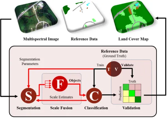
1.2 Proposed Object-Based Classification System with added scale-fusion stage. The process from end to end involves four interwoven stages: Segmentation, Fusion, Classification, and Validation. . . 9
1.3 High resolution image shown at various scales. Note how different structures are prominent at different scales. Al-Masirah Island, Oman. Image courtesy of Digital Globe c . . . 11
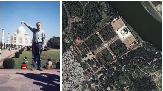
1.4 A strong hierarchy is imposed on size of objects when images are taken from a satellite. Left: Image of a person appearing to be bigger than the Taj Mahal. Right: Image of Taj Mahal from IKONOS satellite. . . 14
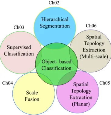
1.5 Thesis is organized into six chapter, all geared to improve object-based image classification. . . 17
2.1 At a very abstract level the semantic object structure of this image is land and water. . . 21
2.2 A scale-tree is the first approximation to the underlying semantic object tree of the image. . . 22
2.3 Major subtasks in spatial processing. It is important to note that in this breakdown, the tasks are not mutually exclusive. For example, description and detection are closely tied together. Having richer descriptions of objects in the image will aid in detection. Likewise, segmentation and representa-tion are also closely tied together.. . . 23
2.4 Object Model : Each region is defined not only by its own properties, but also with the properties of its children. Regions can combine with other adjacent regions to form super-objects and are in turn made up of smaller sub-objects. In this example node 6 and its sub-tree form a rich description of the object represented by that node.. . . 26
2.5 The image on the right is an abstraction of the image on the left. Structures in the image smaller than the specified minimum region size have been hidden. 27
2.6 Abstraction through SCRM i.e. hiding details/regions below a given scale. This mechanism can also be seen as generating segmentations at multiples scales for this specific image. Observing these images, one can see that as the MRS parameter is changed, structures at different scales are brought out. 28
2.7 Hierarchical Scale Space Representation derived using object oriented prin-ciples: Abstraction, Encapsulation, Modularity, and Hierarchy. . . 29
2.8 Scale-tree of a simple image. The underlying segmentations shown in Figure 2.7 . . . 31
2.9 Scale-tree of a simple image. The underlying segmentations shown in Figure 6.3 . . . 31
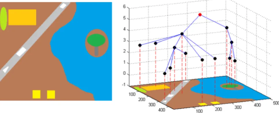
2.10 Scale-tree of a simulated image. The underlying segmentations shown in Figure 2.12 . . . 32
2.11 Scale-tree of a cartoon image simulating the nadir view. See Figure 2.13 to see the simultaneous segmentation and tree view of this image at different levels . . . 32
2.12 Simultaneous tree-segmentation view at different levels for scale-tree shown in in Figure 2.10. . . 34
2.13 Simultaneous tree-segmentation view at different levels for scale-tree shown in in Figure 2.11. . . 35
3.1 Assigning each pixel of the image a label of known class. Image cDigital Globe . . . 36
3.2 The five constructs of a supervised classification task (1) Image (2) Training Set (3) Class Map (4) Testing Set (5) Confusion Matrix . . . 37
3.3 Toy example for computation of confusion matrices . . . 39
3.4 Performance evaluation of support vector machine classifier applied to Uni-versity of Pavia Image (a) Legend (b) Reference Data (c) Color Composite (d) Classification Map . . . 46
4.1 Proposed object-based classification algorithm which starts with the selec-tion of up to n category specific best scales, for a ncategory classification problem. This is followed by an error-minimizing scale fusion stage. In the end, the final class map is obtained by performing a classification of the combined object map. . . 49
4.2 Color composites of the four datasets used in this study: (a) RIT Subset, (b) Rochester Downtown, (c) University Pavia, and (d) Huston Image. . . . 51
4.3 Subsystem view of supervised classification systems: (a) pixel-based, (b) object-based which includes an additional segmentation stage, and (c) Pro-posed: an object-based system with added error modeling. The dotted red lines indicate communication between the subsystems. . . 52
4.4 Consider a a system with perfect ground truth data (eSQSA = 0) and a perfectly trained classifier (eCLS = 0). Without any aggregation (segmen-tation) of the input, this system has zero error. This system will be used to study the impact of increasing aggregation level on the system error. . . 53
4.5 The effect of input aggregation (segmentation) on classification output. No-tice how, under-aggregation does not effect the classifier performance. Also, in rows 4 and 5, you’ll notice that despite of having a perfect classifier the system error is non-zero. Here over-aggregation has impeded the classifiers ability to make the correct decision. We name these misclassifications the over-aggregation-error (eAGG). . . 54
4.6 Consider a a system with high resolution input data but low resolution reference data and a perfectly trained classifier (eCLS = 0). In the absence of aggregation (eAGG = 0), the error of this system arises from mismatch between the very high resolution of input image and low resolution nature of the ground truth. . . 55
4.7 The extra sources of error in an OBC system arising from scale mismatch errors. Over aggregation of input leads toeAGGimpeding the classifier judg-ment while under aggregation brings out the eSQSA which stems from the mismatch between the high resolution classifier output and low resolution ground truth. . . 56
4.8 The best aggregation level for each category is determined through the interaction of the segmentation and the classification subsystems. This step determines the best grain level for each individual category. Selection of the best level is based on maximizing the per-class classification accuracy for that category. . . 58
4.9 Grain and extent at best scales for nine categories of University of Pavia dataset. Each pair of images shows a class map (extent) on the left and its underlying segmentation (grain) on the right. The different granular-ity levels are produced by the levels of a hierarchical segmentation. The sequence presented here, (a) through (i), begins with the coarsest segmen-tation category (Gravel) and ends with the finest segmensegmen-tation category (Trees). Further details of segmentation and classification are provided in 4.5.2. . . 60
4.10 Flow chart of the Fusion Mechanism to obtain a combined object map (COM). Note that the final combined object map contains both coarse and fine grain segments simultaneously. In the zoomed-in areas of final maps, notice how the red category (Bricks) has coarse grain support while the dark green (Trees) category has fine grain support. In essence, the grain for each portion of the map has been tailored to give the best classification for that portion. . . 61
4.11 Boundary placement between categories changes based on the granularity used to make the estimate. Estimates for extent using three different gran-ularity levels are illustrated in (a), (b), and (c). The multi-scale nature of extent is shown in (d), which gives rise to a separation of the image areas into two categories: (e) areas claimed by only one class called the undis-puted territories, and (f) areas claimed by more than one category, conflict zones. . . 63
4.12 Per-Class-Accuracies produced by the algorithms are compared for four data sets. Comparison is between the traditional single scale algorithm (Single Cut) and the multi-cut-and-fused (Proposed). Results of pixel based classification (Pixel-Based) are also included as a baseline. Marker is placed at the mean class accuracy over 10 runs, each with a random selection of training and test data from the ground truth. The ±1 standard deviation from the mean is indicated with the error bars. . . 67
4.13 Analysis of overall accuracy (OA%) over the four data sets. Comparison is between the traditional single scale (SC) algorithm and the multi-cut-and-fused (Proposed). Results of pixel-based classification (PB) are also included as a baseline. The red bar is an average over 10 runs, each with a random selection of training and test data from the ground truth. The blue box shows ±1 standard deviation from the mean. . . 69
4.14 Visual examination of differences between single-cut (SC) and multi-cut-and-fuse (MCF) approach on the Pavia University Image : (a) RGB com-posite, (b) closer look, (c) Extent obtained by SC strategy, (d) Extent obtained by multi-cut-and-fuse strategy, (f) Conflict Zone, (g) Grain from SC approach, (h) Grain from multi-cut-and-fuse approach.. . . 71
4.15 Dataset I - RIT Subset Image - Visual comparison of classification results between the single-cut scale selection approach and proposed multi-cut-and-fused method. In addition, the conflict zone map shows regions where scale-mismatch error exists. . . 76
4.16 Dataset II - Rochester Downtown Image - Visual comparison of classification results between the single-cut scale selection approach and proposed multi-cut-and-fused method. In addition, the conflict zone map shows regions where scale-mismatch error exists. . . 77
4.17 Dataset III - University Pavia Image - Visual comparison of classification results between the single-cut scale selection approach and proposed multi-cut-and-fused method. In addition, the conflict zone map shows regions where scale-mismatch error exists. . . 78
4.18 Dataset IV - Huston Image - Visual comparison of classification results between the single-cut scale selection approach and proposed multi-cut-and-fused method. In addition, the conflict zone map shows regions where scale-mismatch error exists. See Table 4.12 for a color legend of the class map. . . 79
4.19 RIT Subset Image (a) Color Composite (b) Ground Truth . . . 85
4.20 Rochester Downtown Image (a) Color Composite (b) Ground Truth . . . . 86
4.21 University Pavia Image (a) Color Composite (b) Ground Truth. . . 87
4.22 Huston Image (a) Color Composite (b) Ground Truth . . . 88
5.1 Objects appear, as coherent image regions, at different levels. The biggest white object in image (a), is over-segmented in levels 1 & 2, but appears as a coherent region in level 3. . . 91
5.2 Scale-tree corresponding to the image shown in Figure 5.1(a). Each region is displayed as a node. The position of the node on the vertical axis is a function of its position in the scale-space. The scale-tree captures the rela-tionships between regions of the different levels of a multi-scale segmentation. 92
5.3 Eight possible topological configurations between two spatial regions A and B. . . 94
5.4 Illustration of a regions boundary, exterior, and interior obtained from a binary mask of the region. Note that the three elements Ao, A−,and ∂A
are all defined on pixels. . . 95
5.5 Subdivision of the Euclidean space. . . 96
5.6 Dart labeling to define segments. Finite and infinite faces are defined by the direction in which the segments are traversed.. . . 97
5.7 Deriving the permutationσ . . . 97
5.8 Deriving the permutationϕ for a finite face from Figure 5.6a. . . 98
5.9 Deriving the Combinatorial Map of the image. . . 99
5.10 Simple image with regions in various topological arrangements. Note that in (b) only the darts representing the regions are shown to avoid clutter. . . 102
5.11 Closer examination of R4 and R7 . . . 104
5.12 Flow chart to querying topological relationship between two regions using the dart representation . . . 106
5.13 A section of a high-resolution image from WorldView-2 Sensor with a spatial resolution < 0.5m in GSD. Segmentation maps going from fine to coarse details.. . . 106
6.1 Block diagram of overall framework with three main pieces. Pixel to dart conversion, Multi-Scale Region Merging, and Update of data structures that maintain the hierarchy . . . 111
6.2 Illustration of pixel-based support versus dart-based support for a simple image. . . 112
6.3 abstraction . . . 114
6.4 Multi-level segmentation of image. Note that progressively lesser number of darts will be needed to describe the regions as the number of levels go up. This is because going from one level to the next via region merging involves dart removal operations. . . 116
6.5 Recall that the arraysσ andλencode the topology of a single segmentation [70]. Σ and Λ are their multi-dimensional equivalents. In this case, these two arrays encode the segmentation hierarchy shown in Figure 6.4. . . 117
6.6 Encoding and updating ofσ from one level to the next by removal of a dart K={−8}. . . 118
1.1 Basic characteristics of some standard spaceborne sensor instruments [65] . 10
3.1 Performance metrics for toy example . . . 40
3.2 Confusion matrix and computation of the user and producers accuracies . . 40
3.3 Normalized Confusion matrix as a realization ofPX,Xˆ(x,xˆ) . . . 41
3.4 Interpreting the kappa values [55] . . . 42
3.5 Critical values for three commonly used levels of significance. . . 44
3.6 University of Pavia Image Classification Performance . . . 47
4.1 Pairwise statistical significance testing between the algorithms using McNe-mar’s test. The comparison is between single-cut-scale-selection (SC) and multi-cut-and-fuse (Proposed). Middle column SC/Proposed is the column of interest. Comparison with pixel-based is also included for completeness and baseline. Statistically significant differences (zα>1.96) are indicated in bold font. Significance detected in the middle column is also highlighted in red. . . 68
4.2 Overall and per-class accuracies onPavia University data set using recent classification techniques. Comparison is made between pixel based classi-fication (PBC) accuracy and algorithm based classiclassi-fication (ALG). PBC results from spectral information alone, where ALG acts on some com-bination of spatial and spectral information through grouping or spatial regularization.. . . 73
4.3 Performance metrics for dataset I - RIT Subset Image. Highest accuracies are highlighted in bold. Accuracy difference between proposed multi-cut-and-fused approach and the single-cut scale selection approach is shown in the last column. Collective improvement in per-class accuracies, Σ(∆2−1) = 0.83%. . . 80
4.4 Performance metrics for dataset II - Rochester Downtown Image. Highest accuracies are highlighted in bold. Accuracy difference between proposed multi-cut-and-fused approach and the single-cut scale selection approach is shown in the last column. Collective improvement in per-class accuracies,
Σ(∆2−1) = 5.55%. . . 81
4.5 Performance metrics for dataset III - University Pavia Image. Highest ac-curacies are highlighted in bold. Accuracy difference between proposed multi-cut-and-fused approach and the single-cut scale selection approach is shown in the last column. Collective improvement in per-class accuracies, Σ(∆2−1) = 16.94%. . . 81
4.6 Performance metrics for dataset IV - Huston Image. Highest accuracies are highlighted in bold. Accuracy difference between proposed multi-cut-and-fused approach and the single-cut scale selection approach is shown in the last column. Collective improvement in per-class accuracies, Σ(∆2−1) = 24.10%. . . 82
4.7 Segmentation parameters for the four datasets. . . 83
4.8 Parameters for the Scale Fusion stage. Category specific best levels (scales) are selected from the segmentation hierarchy based on performance metric F-1 or PA . Note that either of the metrics can be used for scale fusion but the choice of PA metric yielded best results for the University Pavia image (see Section 4.3.2.1). . . 84
4.9 Classifier training details for the RIT Subset image. . . 85
4.10 Classifier training details for the Rochester Downtown image. . . 86
4.11 Classifier training details for the University Pavia image. . . 87
4.12 Classifier training details for the Huston image. . . 88
5.1 σ encoded as an array of integers indexed by darts. . . 98
5.2 Topology of regions from Figure 5.9(b) encoded as arrays of integers. . . 100
5.3 Topology of regions, from Figure 5.10a, encoded as arrays of integers. . . . 102
5.4 Comparing the time required to generate a region-adjacency-list for all the regions in an image for multiple segmentations. . . 107
6.1 Algorithm for SCRM. . . 113
6.2 Basic algorithm to update permutation σ for each level . . . 118
I Object-Based Classification System 3
1 Introduction 4
1.1 Challenge 1: Accuracy . . . 4
1.1.1 Object Based classification (OBC) . . . 4
1.1.2 Scale Selection Problem . . . 5
1.1.3 Related Work . . . 6
1.1.4 Proposed Solution . . . 8
1.2 Challenge 2: Efficiency . . . 9
1.2.1 Increased Volume . . . 9
1.2.2 Scale and Sensor Diversity. . . 10
1.2.3 Related Work . . . 11 1.2.4 Proposed Solution . . . 12 1.3 Applicability . . . 12 1.4 Context . . . 13 1.5 Research Highlights . . . 15 1.5.1 Conference Publications . . . 15 1.5.2 Journal Publications . . . 16 1.6 Thesis Overview . . . 16 2 Hierarchical Segmentation 19 2.1 Introduction. . . 19 2.2 Motivation . . . 23 2.2.1 Complexity . . . 24 2.2.2 Scale . . . 24
2.2.3 Organization Of Multiscale Information . . . 25
2.3 Proposed Framework and Image Representation. . . 25
2.3.1 Object-based Approach to deal with Complexity . . . 25
2.3.2 Image Region as an Object (Object Model) . . . 26 xi
2.3.3 Mechanism for Encapsulation . . . 27
2.3.4 Dealing with the Organization Issue (scale-tree). . . 28
2.4 Results. . . 30
2.5 Conclusion . . . 32
3 Supervised Classification 36 3.1 Supervised Classification Task. . . 36
3.1.1 The Five Constructs . . . 37
3.2 Evaluation Methodology . . . 38
3.2.1 Toy Example . . . 38
3.2.2 Performance Metrics . . . 40
3.2.3 The Expected Agreement . . . 40
3.2.4 Kappa Coefficient & Its Variance . . . 41
3.3 Significance Testing . . . 43
3.3.1 Better than a Random Classifier?. . . 43
3.3.2 Are Improvements Statistically Significant? . . . 44
3.3.3 Confidence Intervals around ˆκ . . . 45
3.4 Classification of University of Pavia Image . . . 46
4 Scale Fusion 48 4.1 Introduction. . . 48 4.1.1 Objectives . . . 48 4.1.1.1 Proposed Algorithm . . . 48 4.1.1.2 Original Contributions . . . 49 4.1.2 Chapter Organization . . . 49 4.2 Study Areas . . . 50 4.3 Methods . . . 51
4.3.1 A model for Scale-Mismatch Errors in an OBC System. . . 51
4.3.1.1 Over-Aggeregation Error (eAGG) . . . 52
4.3.1.2 Scale-of-Question-Scale-of-Answer Error (eSQSA) . . . 54
4.3.1.3 Hierarchical Segmentation and OBC Errors . . . 55
4.3.2 Proposed Algorithm: Eliminating Scale-Mismatch Errors through Scale Fusion. . . 57
4.3.2.1 Category Based Characteristic Scale Selection . . . 57
4.3.2.2 Fusion Mechanism . . . 60
4.3.3 Evaluation Method . . . 64
4.4 Results. . . 66
4.4.1 Per-class Performance Evaluation . . . 66
4.4.2.1 Overall Accuracy (µ±σ ) . . . 68
4.4.2.2 Statistical Significance. . . 68
4.4.3 Visual Evaluation: Class Maps and Conflict Zones . . . 70
4.4.4 Additional Performance Metrics . . . 72
4.4.5 Benchmarking . . . 73
4.5 Conclusions . . . 74
4.5.1 Addendum to Results . . . 76
4.5.1.1 Classmaps for the Four Datasets . . . 76
4.5.1.2 Tables of Accuracy Metrics . . . 80
4.5.2 Experimental Details. . . 82
4.5.2.1 Hierarchical Segmentation . . . 82
4.5.2.2 Scale Fusion Mechanism. . . 83
4.5.2.3 Supervised Classification . . . 85
II Efficient Spatial Information Extraction 89 5 Encoding of Topological Information 90 5.1 Introduction. . . 90
5.2 The Region Connection Calculus Model . . . 93
5.3 The Combinatorial Maps Model (CM). . . 95
5.3.1 The CM Model Definitions . . . 96
5.3.2 Applying the CM Model to Image Regions . . . 98
5.3.3 Querying Topological Adjacency & Containment . . . 100
5.4 Results and Discussion . . . 101
5.4.1 Example Image and it’s Dart-based Representation . . . 102
5.4.2 Deriving the RCC-8 Relationships Using The CM Model . . . 103
5.4.3 Querying the topology of any two regions Ri and Rj . . . 105
5.4.4 Performance Comparison . . . 105
5.5 Conclusions and Future Work . . . 107
6 Discrete Topology for Multiple Scales 109 6.1 Abstract . . . 109
6.2 Introduction. . . 109
6.3 Framework Based on Discrete Topology . . . 111
6.3.1 Conversion from Pixels to Darts . . . 112
6.3.2 Merging Mechanism to Generate a Hierarchy . . . 113
6.3.3 Data Structures & Procedures to Encode the Hierarchy . . . 114
6.3.3.2 Update of LAMBDA (Λ) . . . 119
6.4 Results. . . 119
6.5 Conclusions . . . 120
7 Conclusions & Future Work 121 7.1 Contributions . . . 122
7.1.1 Conference Publications . . . 123
7.1.2 Journal Publications . . . 123
Abdul Haleem Syed
Submitted to the
Chester F. Carlson Center for Imaging Science in partial fulfillment of the requirements
for the Doctor of Philosophy Degree at the Rochester Institute of Technology
Abstract
Land-use-and-land-cover (LULC) mapping is crucial in precision agriculture, environ-mental monitoring, disaster response, and military applications. The demand for improved and more accurate LULC maps has led to the emergence of a key methodology known as Geographic Object-Based Image Analysis (GEOBIA). The core idea of the GEOBIA for an object-based classification system (OBC) is to change the unit of analysis from single-pixels to groups-of-single-pixels called ‘objects’ through segmentation. While this new paradigm solved problems and improved global accuracy, it also raised new challenges such as the loss of accuracy in categories that are less abundant, but potentially important. Although this trade-off may be acceptable in some domains, the consequences of such an accuracy loss could be potentially fatal in others (for instance, landmine detection).
This thesis proposes a method to improve OBC performance by eliminating such accu-racy losses. Specifically, we examine the two key players of an OBC system : Hierarchical Segmentation and Supervised Classification. Further, we propose a model to understand the source of accuracy errors in minority categories and provide a method called Scale Fusion to eliminate those errors. This proposed fusion method involves two stages. First,
tation and supervised classification. Next, these estimated scales (segmentation maps) are fused into one combined-object-map. Classification performance is evaluated by com-paring results of the multi-cut-and-fuse approach (proposed) to the traditional single-cut (SC) scale selection strategy. Testing on four different data sets revealed that our pro-posed algorithm improves accuracy on minority classes while performing just as well on abundant categories.
Another active obstacle, presented by today’s remotely sensed images, is the volume of information produced by our modern sensors with high spatial and temporal resolution. For instance, over this decade, it is projected that 353 earth observation satellites from 41 countries are to be launched. Timely production of geo-spatial information, from these large volumes, is a challenge. This is because in the traditional methods, the underlying representation and information processing is still primarily pixel-based, which implies that as the number of pixels increases, so does the computational complexity. To overcome this bottleneck, created by pixel-based representation, this thesis proposes a dart-based discrete topological representation (DBTR), where the DBTR differs from pixel-based methods in its use of a reduced boundary based representation. Intuitively, the efficiency gains arise from the observation that, it is lighter to represent a region by its boundary (darts) than by its area (pixels). We found that our implementation of DBTR, not only improved our computational efficiency, but also enhanced our ability to encode and extract spatial information.
Overall, this thesis presents solutions to two problems of an object-based classifica-tion system: accuracy and efficiency. Our proposed Scale Fusion method demonstrated improvements in accuracy, while our dart-based topology representation (DBTR) showed improved efficiency in the extraction and encoding of spatial information.
Object-Based Classification
System
Introduction
This thesis presents solutions to two problems of an object-based classification system: accuracy and efficiency. Section1.1, presents introduction and background to the accuracy problem. Followed by Section 1.2, which provides background on the efficiency problem. Section1.3, discusses the applicability of our proposed methods. Section1.5, highlights our research contributions. Finally, Section1.6, presents an overview and thesis organization.
1.1
Challenge 1: Accuracy
1.1.1 Object Based classification (OBC)
Land-use-and-land-cover (LULC) mapping is crucial in precision agriculture, environmen-tal monitoring, disaster response, and military applications [38]. The demand for improved and more accurate LULC maps has led to the emergence of a key methodology known as Geographic Object-Based Image Analysis (GEOBIA). The core idea of the GEOBIA for an object-based classification system (OBC) is to change the unit of analysis from single-pixels to groups-of-pixels called ‘objects’ through segmentation [2][17]. Among other things, this
approach solved the paradox of lowered classification accuracy with use of successively higher spatial resolution data that was observed as sensor technologies improved. This was because ‘objects’, when acted upon as a unit, shielded the high variability of individ-ual pixels from the classifier leading to better performance [56]. While the new paradigm solved problems, it also raised new challenges such as thescale selection problem.
1.1.2 Scale Selection Problem
The scale selection problem is the challenge of deciding on an appropriate level of pixel grouping to yield meaningful objects, where the amount of grouping dictates the size (scale) of the objects produced. In practice, scale selection in an OBC system translates to the issue of segmentation-parameter selection [53, 36, 72, 34, 42, 47]. In [16], Blashke noted that defining a scale parameter for segmentation is the most difficult and problematic is-sue. This is because high-resolution remotely-sensed images generally contain information simultaneously at several scales, all embedded in one spatial layer often without any a priori scale knowledge. A target of interest may be a rare occurrence (needle in a hay stack) or an abundantly repeating object (e.g. buildings in urban scenes). Alternatively, an analyst may be interested in monitoring a much larger entity such as an industrial compound. Hence, a single-best-scale solution that serves all categories of interest has been elusive.
This can be seen from classification results of some recent publications on a widely used hyperspectral data set (Pavia University Image). For instance, [8] proposed a multi-scale conditional random field framework for region based classification, which improved overall accuracy by 12.2% compared to a baseline pixel-based classification (PBC). How-ever, individual accuracies forTrees and Shadows category were lost by 12.2% and 2.1% respectively. In another case, authors of [43] proposed a spatial-spectral method that incorporates morphological attribute profiles to account for spatial dependencies. Their
method improves overall accuracy by 17.5%, however, 6.2% accuracy is lost in the Shad-ows category. In both cases, although the overall accuracy increased, the less abundant categories lowered in accuracy compared to the original pixel-based result. A similar pat-tern was also observed in results reported by [52, 38]. In these instances, a 2% loss in accuracy of Trees category seems harmless, however the consequences of such a loss in
Landmine detection accuracy could be potentially fatal [80]. This raises the question, for the minority class results, what is the source of errors (misclassifications)?
Modeling of error sources within an OBC system is still in its infancy. For instance, its known that an OBC system has three subsystems: Segmentation, Classification, and Validation. Yet, it is common practice to report one lumped overall accuracy metric (OA% = 1- Error%) [60, 4, 51]. This provides no indication as to whether the error is from segmentation or the classification stage. Visa and Salembeir point out that making such a distinction is important because ignoring the quality of the segmentation can lead to biased results [77]. For the four cases presented, [52,8,43,38] , within each individual reference, the same classification mechanism (training, testing, & classifier) was used for both the baseline (PBC) and their proposed algorithm; therefore it is likely that these errors are being introduced from the segmentation stage (grouping, spatially regularizing). A method to eliminate these segmentation stage errors has recently been proposed. It involves choosing, not one, but appropriate segmentation scales for all distinct categories of interest and intelligently combining them.
1.1.3 Related Work
Recently, Sellaouti et al. proposed a hierarchical classification based Region growing (HCBRG) method where segmentation and classification collaborate to determine the fi-nal classification map [66]. The HCBRG algorithm overcomes the limitations of region merging by deriving high quality seeds and growth criterion cues from the supervised
classification step. It intelligently avoids the single-best-scale selection problem through iterative collaboration between segmentation and classification. However, this technique does not explicitly determine the best segmentation scale for each category thereby provid-ing estimates for only a classification map (extent) and not the underlyprovid-ing segmentation (grain).
Authors of [85,83,82] overcome this challenge with their multi-granularity synthesis segmentation method. Like [66], their segmentation and classification work in collabora-tion, the process starts based on the initial classificacollabora-tion, where the image is divided into mutually exclusive land category masks. Appropriate scale of aggregation is determined for each mask (category). Merging is stopped when classification accuracy for each cat-egory is maximized. Finally, the masked regions are combined into a unified map which provides both segmentation (grain) and classification (extent). The challenge with this approach is that, although grain was discovered through multiple scales (region merging levels), the extent was determined only at a single scale (pixel level). This implies that such a methodology may perform well farther away from the boundaries, but the performance at the boundaries has not been optimized at appropriate category scales.
In the methods referenced thus far, we note that some aspects of scale were modeled while others were not. For instance, category extent was modelled by [66] , but grain was neglected. The opposite was true in [85, 83, 82], where grain was modelled at multiple scales while the extent was not. Our proposed approach differs from such methods in its use of a more complete description of scale, based on principles from Landscape Ecology. The following concepts are of particular interest : Characteristic Scale, Grain, Extent, and Transition Zones. Turner et al. [75] asserted that avoiding scale mismatch errors requires explicit consideration of the characteristic scale of each phenomenon of interest, where a characteristic scale is the scale at which a pattern or an ecological phenomenon principally operates (Figure1.1).
(a) Three Categories (b) Category Grain (c) Category Extent
Figure 1.1: Consider an image with three categories A,B, and C. Each category is characterized by
its own uniquegrain andextent. In this illustration Category A has fine grain support, Category
B has medium grain, while Category C is defined on a coarser grain.
A full specification of a characteristic scale requires specifying both its grain and extent; where grain is the size of the individual units of observation i.e. the smallest entities that can be distinguished [79] and extent defines the spatial span of the population we wish to sample [81]. Together, these components define the upper (extent) and lower (grain) resolution limits of a study. Finally, the exact appearance of boundaries (extent), changes depending on the scale of observation. Woodcock and Strahler [81] observed that classes in most environment are not pure, especially at the transition area from one category to the next. Therefore, although characteristically different, at the transition the two classes grade together subtly, with all combinations occurring in the middle [81], these areas of transition can be designated as transition zones. Unlike the prior art, we explicitly model these concepts of grain, extent, and transition zones in our algorithm ; with the objective of minimizing the scale mismatch errors.
1.1.4 Proposed Solution
To overcome the challenges highlighted thus far, we formulate the OBC problem as that of multiple-scale-selection followed by error-minimizing-fusion. Our objective is to test the hypothesis that, for a supervised classification task, scale-combination outperforms single-scale-selection. We postulate that minority category accuracy errors are related to the scale selection problem, specifically, it’s manifestation inside of an OBC system.
Further we postulate that explicitly considering the characteristic scale of each category will minimize errors and improve performance globally while preserving accuracy of less abundant categories.
Figure 1.2: Proposed Object-Based Classification System with added scale-fusion stage. The
process from end to end involves four interwoven stages: Segmentation, Fusion, Classification, and Validation.
1.2
Challenge 2: Efficiency
1.2.1 Increased Volume
With rapid developments in satellite and sensor technologies, there has been a dramatic increase in the availability of high resolution (HR) remotely sensed images. For example,
the WorldView-2 sensor can capture images at<0.5mresolution with a collection capacity of 300,000 sq mi/day (See Table 1). At this rate, this instrument alone can cover the entire USA in 12 days. It is projected that 353 earth observation (EO) satellites will be launched in this decade as compared to 33 in the previous decade [1]. Hence, the ability to collect images remotely is expected to far exceed our capacity to analyze these images manually. Consequently, techniques for assisted analysis are urgently needed to support analysts in generating effective results in an efficient and timely manner.
1.2.2 Scale and Sensor Diversity
Apart from the increased volume, another important facet which adds to the complexity of the problem is the wide diversity of the acquired data from different sensors: SAR, LIDAR, infrared, electro-optic, etc. These instruments cover a wide range of spatial, spectral and temporal resolutions. Therefore, there is a growing need for multi-sensor fusion algorithms capable of seamlessly integrating data for improved quality [57]. Advances in information fusion have surfaced in other domains such as medical imaging [78], where MRI, fMRI, and PET modalities have been combined to assist radiologists in providing more accurate diagnosis. However, such techniques are not directly applicable to remotely sensed imagery due, in part, to the wide variability of the scale at which these images are captured (See Figure1.3 for a brief illustration).
Table 1.1: Basic characteristics of some standard spaceborne sensor instruments [65]
Instrument Bands Ground Spot Distance (Spatial) Revisit Rate (Temporal) Landsat TM 7 30 m , 120 m 16 days
QuickBird 5 2.44 m, 0.61 m 1 - 5 days
AVHRR 5 1.1 km 0.5 day
Figure 1.3: High resolution image shown at various scales. Note how different structures are
prominent at different scales. Al-Masirah Island, Oman. Image courtesy of Digital Globe c
This issue is precipitated, in general, by the extensive range of sizes/scales at which objects of interest may appear in HR remotely sensed images. A target of interest may be a rare occurrence (needle in a hay stack) or an abundantly repeating object (e.g. buildings in urban scenes). Alternatively, an analyst may be interested in monitoring a much larger entity such as an industrial compound. This wide variation in scale contributes significantly to the complexity of the problem. High resolution remotely sensed images generally contain information simultaneously at several scales; all embedded in one spatial layer often without any a priori scale knowledge. Traditional linear-scale-space techniques attempt to create multi-scale representations by creating a stack or pyramid, where a given level is generated by down-sampling a higher resolution version [64]. Since these techniques address more than one scale they have an inherent advantage over single-segmentation-output methods. However, these methods have yet to address two main challenges. First, the number of scales needed in a stack to represent any given image is generally unknown. Using a regularly sampled stack will often result in lost information and may also generate levels that contain no relevant information. Second, the down sampling mechanism often gives rise to blurred edges/images. Consequently, an improved scale-space representation is needed to effectively handle the above described problem.
1.2.3 Related Work
Several Multi-scale techniques have been proposed to address the aforementioned issues (See [32] for a comprehensive survey). These multi-scale representations are hierarchical
in nature and are derived through various groupings of homogeneous image pixels/regions in the feature space. Commonly used features for grouping are spectral signatures, tex-ture and shape. A multi-resolution/hierarchical segmentation was proposed in [11], where the process of generating a hierarchy starts with each pixel as an object and then succes-sively merges additional pixels based on criteria of similarity and homogeneity. A similar approach was proposed by [84], where multi-scale segmentations were used to synthesize coherent ground objects. The above mentioned techniques tackle the issue of scale through multi-scale segmentation; but do not leverage topological features as in [70][49] or address the scalability of their representation to images from multiple sensors. Hence, a frame-work of image analysis is needed to tackle the issues of scale, complexity and information organization at the initial stages of the processing chain rather than dealing with these issues at later stages.
1.2.4 Proposed Solution
To overcome the above mentioned issues, we propose a framework for a discrete topology based multi-scale segmentation of high resolution satellite images. This proposed rep-resentation builds-on and improves our previous research on scale-space reprep-resentation [69] and topological information extraction and encoding [70]. Our goal is to provide an effective foundation/framework that will facilitate/assist analysts in tasks such as tar-get detection/recognition, classification, change detection, and multi-sensor information fusion.
1.3
Applicability
The significance of this research is primarily embedded in its ability to advance a framework that utilizes multi-scale segmentations, and topological features to characterize
informa-tion in a hierarchical representainforma-tion. Its primary goal is to assist analysts in effectively and efficiently process scenes for intelligence purposes.
• Organization and sorting of a large area scene: The proposed research will give the analyst an ability to sort the image content by scale in an intuitive representation that allows for better comprehension of the scene. It will enable rapid sifting of the hierarchy in order to find and focus on appropriate object resolution levels for a given task, i.e., looking for an automobile vs. a building.
• Query of topological information: The proposed work will provide the analyst the ability to query topological relationships i.e., finding out what objects are included or adjacent in a given area/object of an image. This provides the analyst with a way to perform analysis on the surroundings of an object-of-interest, thereby incorporating contextual information in the decision making process.
• Multi-sensor data fusion: This research will provide a unified framework to com-bine information from multiple sensors into a common representational format. The benefits of multi-sensor fusion will include increased spatial and temporal cover-age, increased robustness to sensor failures, better noise suppression and increased estimation accuracy.
1.4
Context
As discussed earlier, segmentation is a key step in the object-based image analysis chain. As a result, the literature presents a plethora of approaches to solve the segmentation problem. Many times the segmentation approach adopted is dictated by the application domain. For satellite images, the class of segmentation methods that fall under the “Hier-archical Segmentation” type are particularly well suited. This is because the large distance
between the satellite and objects being imaged imposes a perspective where relative size between the objects is preserved.
Figure 1.4: A strong hierarchy is imposed on size of objects when images are taken from a satellite. Left: Image of a person appearing to be bigger than the Taj Mahal. Right: Image of Taj Mahal from IKONOS satellite.
Satellite images maintain a strict hierarchy on the size of objects that appear in them. That is, a building, which is a physically bigger object, will appear bigger than a person, a physically smaller object. This is not always the case with regular images. For instance, in Figure1.4, given the perspective of the first image, a human appears bigger than the Taj Mahal, and the relative size of the objects is not preserved. However, such a distortion is not possible from the satellite image view (Figure 1.4, Right). This observation of strict hierarchy on size also provides the intuition for Size-Constrained-Region-Merging algorithm presented in Chapter 2.
1.5
Research Highlights
Key contribution of this thesis are:
1. Application of Landscape Ecological concepts to segmentation and classification 2. A model to understand scale-mismatch errors
3. Category-aware scale detection and fusion for eliminating errors 4. Spatial localization of scale-mismatch errors
5. Improved accuracy in less-abundant and fine-grained categories
6. Algorithm for spatial topology extraction using combinatorial math model 7. Implementation of discrete topological framework for remotely sensed images 1.5.1 Conference Publications
1. Y. Hu, A.H.Syed, E. Saber, N. Cahill, and D. Messinger, “Dynamic scale-space representation based on a MRF region merging model,” GEOBIA 2014
2. Y. Liang,A.H.Syed, N. Cahill, E. Saber, D. Messinger,“Application of Tree Match-ing Techniques to High Resolution Remotely Sensed Images towards Object Detec-tion,” GEOBIA 2014
3. A.H.Syed, E. Saber, and D. Messinger,“Discrete Topology Based Hierarchical Seg-mentation for Efficient OBIA : Applications to Object Detection in Satellite Images,” ISPRS 2013
4. A.H.Syed, E. Saber, and D. Messinger,“Encoding of Topological Information in Multi-Scale Remotely Sensed Data: Applications to Segmentation and OBIA,” GEO-BIA 2012 (Best Paper Award)
5. A.H.Syed, E. Saber, and D. Messinger, “Scale-Space Representation of Remotely Sensed Images using Object-Oriented Approach, ” SPIE 2011
1.5.2 Journal Publications
1. A.H.Syed, N. Cahill, D. Messinger, Y. Liang, and E. Saber, “Category-Aware Scale Fusion Improves Object-Based Classification: A Solution to the Scale Selection Prob-lem,” Journal of Remote Sensing of Environment 2015 (Submitted May 5th) 2. A.H.Syed, N. Cahill, D. Messinger, Y. Liang, and E. Saber, “The Effect of Object
Definition on Object-Based Classification Accuracy: A Study,” Journal of Remote Sensing of Environment 2015 (In Preparation)
1.6
Thesis Overview
The first three chapters are aimed at improving the accuracy aspect of an object-based classification system:
Chapter 2presents the derivation of a Hierarchical Segmentation based on the princi-ples of object-based image analysis. The hierarchical scale-space representation is designed to meet the challenges, of complexity, scale, and organization, that are often associated with high resolution remotely sensed images. Elements of the representation such as ob-ject definition and encapsulation mechanism are described. Followed by demonstration of the hierarchical segmentation on some synthetic and real images.
Chapter 3 presents supervised classification and its evaluation methodology. First, a brief review of supervised classification of remotely sensed images is included. Followed by details on the evaluation methodology and statical significance testing. Performance evaluation method for an individual algorithm, as well as, comparison between different algorithms is discussed.
Figure 1.5: Thesis is organized into six chapter, all geared to improve object-based image classi-fication.
Chapter 4 builds on the previous chapters and details two important aspects of this thesis: a model for scale-mismatch errors, and a scale fusion method to eliminate those errors. Performance of our proposed algorithm is tested on four different datasets and results are presented in detail.
The remaining two chapters are aimed at solving the efficiency problem, which arises from a pixel-based representation/processing of image regions:
Chapter 5 presents an introduction to the traditional Region Connection Calculus (RCC-8) model for spatial information extraction. An improved combinatorial map (CM) model for image representation is implemented which is based on reduced boundary based
representation (darts). Performance is compared pixel-based (RCC-8) and dart-based (CM) approaches. An algorithm to query and categorize spatial arrangement is also proposed.
Chapter 6builds on the model presented in the previous chapter for a single scale and extends it to multiple scales. Data structures and algorithms required for implementation and facilitation of multi-level topological queries are discussed. Finally, the multi-level discrete topology based framework is applied to hierarchical segmentation of remotely sensed images via the Size Constrained Region Merging (SCRM) algorithm.
Hierarchical Segmentation
2.1
Introduction
With rapid developments in satellite and sensor technologies, there has been a dramatic increase in the availability of high resolution (HR) remote sensing images (<1m). There is a growing need for automated image analysis techniques which go beyond the traditional pixel based methods (spectral), many of which do not leverage the abundant spatial, contextual, and topological information that is now available in HR images. The HR image brings with it several challenges. It is highly complex with relevant structures occurring at several scales. A single segmentation or image representation may not capture all the information present in the image and thus requiring multi-scale techniques. To deal with complexity and organization of multi-scale information, a consistent framework and image representation is needed.
To solve the larger problem of automated or assisted image analysis, first the image must be represented appropriately. This implies that rather than using the inherent pixel representation which is dictated by the capturing device, we would like the image to be
mapped onto objects that are meaningful entities in the problem domain. Therefore, for our purpose an ideal image representation has five main properties among others: (1) has building blocks that are meaningful entities in the problem domain, (2) accounts for structures at different scales (3) has the ability to incorporate expert/domain knowledge into the representation, (4) lends itself to analysis using the state of the art techniques from probabilistic graphical models, and finally (5) requires minimum to no manual parameter tuning.
We propose an object-based scale-space image representation (hierarchical segmenta-tion) which is designed with the above mentioned properties in mind. An object-based approach is used where the principles of abstraction, encapsulation, modularity and hi-erarchy are observed. These principles will be explained briefly in section 2.3.1. Object-based design offers several advantages over heuristic design approaches especially when the problem is complex. For example, an object-based design offers economy of expression by restating the problem, into entities (objects) that are specific to the problem domain [18]. More importantly an object-based design approach offers a foundational framework that facilitates our understanding of the problem and the solutions to it.
Figure 2.1: At a very abstract level the semantic object structure of this image is land and water.
Before proceeding, we would like to clarify our usage of the terms the scale-tree and
object-tree. In the context of this thesis, a scale-tree (section 2.3.4) is the data structure that contains the scale-space breakdown of the image and the term object-tree is used to describe the data structure that captures the high-level interpretation (semantic break-down) of the image. At a very abstract level, the semantic object structure of the image in figure2.1 can be summarized by the words land and water. But for any given image, the mapping between low level features such as color, texture, shape etc.. and the high level semantic object breakdown is non-trivial. As such, any representation derived on the basis of low-level features alone can not be assumed to be the true underlying seman-tic object structure. The aim of this chapter is to derive the scale-tree, a representation based on low-level features, which will serve as an initial approximation to the underlying object-tree (see Figure2.2).
The remainder of this chapter is organized as follows. Section 2.2 explains our mo-tivation to design a coherent image representation. Section 2.3 describes our proposed approach and its similarity/differences from other works. Section 4 shows examples of our
Figure 2.2: A scale-tree is the first approximation to the underlying semantic object tree of the image.
2.2
Motivation
Our strategy in designing tools for assisted image interpretation/analysis has a spectral side and a spatial side. The focus of this chapter will be on the spatial processing. The major tasks involved on the spatial processing can be grouped under the following three areas: Segmentation, Description, and Detection (Figure2.3). In our initial attempts at solving the problems of Detection and Segmentation, a key issue that surfaced repeatedly isimage representation. We found it necessary, as will be explained in the remainder of this section, to include image representation as a major subtask of spatial processing. When processing high resolution satellite images one is commonly faced with the problems of complexity, scale and organization. These issues are described here to illustrate the need for a coherent framework to solve them.
Figure 2.3: Major subtasks in spatial processing. It is important to note that in this breakdown, the tasks are not mutually exclusive. For example, description and detection are closely tied together. Having richer descriptions of objects in the image will aid in detection. Likewise, segmentation and representation are also closely tied together.
2.2.1 Complexity
Traditional Anomaly/Outlier detection techniques require recognition of normal instances to detect an instance that is anomalous. Typically, these techniques are based on assump-tions that may not always hold true. Furthermore, these techniques are not designed to make comparisons across different scales. The order and scale of the data under examina-tion is assumed to be roughly the same. High resoluexamina-tion remotely sensed images (HRRS), resolution <0.5m, have an overwhelming amount of detail and are inherently complex. Therefore, before existing detection techniques can be utilized, the problem of complexity of the image must be solved via decomposition of information (image) into manageable pieces.
2.2.2 Scale
HRRS images contain information simultaneously at several scales all embedded in one spatial layer and there is no prior information as to what those scales are. Traditional linear-scale-space techniques attempt to create multi-scale representations, by creating a stack or a pyramid, where each level is generated by down-sampling the level below it [64]. A similar approach is used in a well-known Visual Saliency Model introduced by Itti, Kotch & Niebur. In this model, which predicts visually salient regions of a given image, only nine spatial scales are utilized to deal with the issue of scale [50]. There are two main problems with such a representation. First, the number of scales needed in a stack, to represent any given image, is an unknown. Also, using a regularly sampled stack will result in lost information and will generate levels in the stack where there is no relevant information, if none existed in the original image. Second, the down-sampling mechanism, convolution with a Gaussian kernel, that is used to generate each level, gives rise to problems of blurred edges. More importantly, information on topological relationships between objects such as
containment and adjacency are not utilized going from one level to the next in traditional scale-space models.
2.2.3 Organization Of Multiscale Information
Assuming the issues of complexity and scale are solved i.e. the given complex image is successfully decomposed and information at all relevant scales is successfully derived, some questions still remain to be answered. How is this copious amount of information going to organized and stored? How can we best arrange this information so as to facilitate the tasks of segmentation, description and detection? These questions need to be answered within the constraints imposed by physical implementation.
2.3
Proposed Framework and Image Representation
Our proposed representation involves four steps : (1) using an object-based approach to reduce complexity, (2) defining an object model, (3) establishing an mechanism for encapsulation, and (4) using a scale-tree for organizing the information.
2.3.1 Object-based Approach to deal with Complexity
To deal with the complexities described thus far, an object oriented approach is utilized. This approach is motivated by leveraging the knowledge on how complex systems in other disciplines are organized. According to Booch, an object-oriented-solution to solve a com-plex problem follows four major principles: Abstraction, Encapsulation, Modularity and Hierarchy [18]. Each of these four principles helps reduce complexity and facilitate un-derstanding. Abstraction and Encapsulation complement each other. Abstraction entails keeping only those unique characteristics of an object that separate it from others, while Encapsulating (hiding) all other details not relevant to the task at hand. Modularity is
grouping together of similar abstractions, while Hierarchy is about bringing order and organizing all the different levels of abstractions according to some criteria.
Figure 2.4: Object Model : Each region is defined not only by its own properties, but also with the properties of its children. Regions can combine with other adjacent regions to form super-objects and are in turn made up of smaller sub-objects. In this example node 6 and its sub-tree form a rich description of the object represented by that node.
2.3.2 Image Region as an Object (Object Model)
An image region can be seen as an object that has the following defining characteristics: Boundary, State, Identity, and Behavior [18]. These defining characteristics are briefly explained here. An object has finite spatial extent and boundaries that separate it from other objects. Thestate of an object encompasses all of the (usually static) properties of the object plus the current (usually dynamic) values of each of these properties. For this chapter only the static properties are considered. Theidentity of an object is a property that is an inherent characteristic that contributes to making an object uniquely that
object. For instance, in an image, it is usually assumed that distinct objects in the scene appear as relatively homogeneous patches of the same color (spectral signature). Finally the behavior of an object can be stated in terms of how it interacts with its topological neighbors to form a super object while the object itself is made up of smaller sub-objects (see Figure2.4).
2.3.3 Mechanism for Encapsulation
To realize this object model through the principles of object oriented design, a mechanism for Encapsulation (information hiding) called Size-Constrained-Region-Merging (SCRM) is used. SCRM allows us to create more abstract representations of a region. This is done by eliminating all the regions in a given image that are smaller than specified scale [23]. Figure2.5demonstrates the parameter that controls the level of abstraction using SCRM.
Figure 2.5: The image on the right is an abstraction of the image on the left. Structures in the image smaller than the specified minimum region size have been hidden.
A stack of images with decreasing level of detail can be generated by sweeping the parameter Minimum Region Size (MRS) going from 1 pixel to N pixels (where N is the total number of pixels in the image). The stack of images in Figure 6.3, is a suite of segmentations of the image ordered by the level of detail present in the image. Objects that are hidden at each level can be isolated by taking a difference between any two consecutive levels.
Figure 2.6: Abstraction through SCRM i.e. hiding details/regions below a given scale. This mechanism can also be seen as generating segmentations at multiples scales for this specific image. Observing these images, one can see that as the MRS parameter is changed, structures at different scales are brought out.
2.3.4 Dealing with the Organization Issue (scale-tree)
The scale-tree is used to store and organize all the structures present at different scales in an image. A similar data structure, called the segmentation-tree, is used by references [71,5]. In their work the multi-scale information is derived through a non-linear transform that performs integrated edge and region detection. We borrow the term scale-tree from [13,45] where the scale space of the image is derived using a morphological operator called sieve [12]. The sieve operator is a combination of morphological opening and closing. This representation overcomes the two problems (section2.2.2) associated with the linear-scale space representation. First, the image is sieved going from the smallest possible object (1px) up to the maximum size of the image, while leaving out scales where no objects are present. Second, the topological relationships such as containment and neighborhood are derived and recorded while going from one level to the next.
However, in our proposed representation, the scale-tree is derived differently by using SCRM [23] which we describe in section 2.3.3. SCRM allows the regions/structures to evolve, from one level to the next, without any restrictions on their shape. The boundary
of the new region formed is an aggregate of boundaries of regions in the level below. This preserves the integrity of the boundary in the stack, as no information loosing operations such as blurring are being applied. The final scale-tree generated using the above tools is, an arrangement of image regions in, a hierarchy by size and containment relationships. The overall representation obeys the four principles of object oriented design as illustrated in Figure2.7. and the final scale-tree generated using the above tools is an arrangement of image regions in a hierarchy by size and containment relationships.
Figure 2.7: Hierarchical Scale Space Representation derived using object oriented principles:
2.4
Results
This section presents the results of testing our proposed representation on simple (syn-thetic) and real satellite images. The results can be visualized from two different points of view: The tree view and the segmentation view. The tree view brings out relationships between the structures of the image allowing us to see how the structures at different scales are arranged, without any details on their geometry. The segmentation view, on the other hand, is a collection of all the segmentations going from fine to coarse. This suite of segmentations can be navigated to find the level of interest, offering a view of the geometry of all the regions contained in that level.
In the following visualizations of the scale-tree, each region is represented by a node (Figure2.8,2.9, 2.10,2.11) in the tree. The position of the node on the x-y plane is the centroid of the region. The position of the node on the vertical axis is a function of its position in the scale-space and its topology. The root node, red, indicates the entire image while the leaf nodes of the tree are the smallest regions. Each level of the tree is made up of regions of size greater than regions in the level below it. This can be observed when examining the segmentation map associated with a particular depth in the scale-tree as shown in Figures 12 and 13 in the Appendix.
Figure 2.8: Scale-tree of a simple image. The underlying segmentations shown in Figure2.7
Figure 2.10: Scale-tree of a simulated image. The underlying segmentations shown in Figure2.12
Figure 2.11: Scale-tree of a cartoon image simulating the nadir view. See Figure2.13to see the
simultaneous segmentation and tree view of this image at different levels
2.5
Conclusion
Challenges faced during spatial processing of high resolution remotely sensed images have been explained (complexity, scale, and organization). An object-oriented framework to solve these problems was presented. An image or image region was treated as an object which can be represented at different levels of abstraction by encapsulating or controlling the level of detail. The different levels of abstractions were organized in a scale-tree to form a hierarchy by size and topological relationships of adjacency and containment. Our final representation, the scale-tree, contains the scale-space of the image storing inside it segmentations of varying levels of detail.
The proposed representation gives us a foundation on which subtasks of description and detection can be performed. The nodes of the scale-tree serve as a natural representation of regions of the image. The scale-tree will form the backbone on which probabilistic models will be superimposed. Treating the nodes of the tree as random variables and characterizing their interactions will help uncover the underlying semantic object structure of the image.
Figure 2.12: Simultaneous tree-segmentation view at different levels for scale-tree shown in in
Figure 2.13: Simultaneous tree-segmentation view at different levels for scale-tree shown in in
Supervised Classification
A pertinent review of the supervised classification, in the context of remotely sensed images, is presented here in four parts: (1) Definition and Terminology, (2) Performance Metrics and Toy Example (3) Statistical Significance Testing, and (4) Example on a real image.
Figure 3.1: Assigning each pixel of the image a label of known class. Image cDigital Globe
3.1
Supervised Classification Task
The goal of the classification task is to discriminate between different land cover types present in a scene. To accomplish this, each pixel of the image is assigned to known
thematic classes that exist in the scene, such as land or water. The assignment is done automatically by a classifier which has been trained on a small set of ground truth pixels. Both the training and evaluation procedures are dependent on accurately labelled data, therefore the ground truth pixels are collected through a supervised process by a trained analyst who carefully designates pixels that belong to known land cover types.
Figure 3.2: The five constructs of a supervised classification task (1) Image (2) Training Set (3) Class Map (4) Testing Set (5) Confusion Matrix
3.1.1 The Five Constructs
Image classification is a broad area, spanning several disciplines, each of which has its own terminology. In order to avoid confusion, the five fundamental constructs of supervised classification are presented here, as they are commonly used in the remote sensing field.
1. Image: The input image is a multi/hyper-spectral image collected by the satel-lite. For example, an image collected by the LANSAT Thematic Mapper collects information at seven different wavelengths, resulting in a seven band image.
2. Training Set: The training set is a subset of pixels with known labels which will be used to train the classifier.
3. Class Map: The output of the classification process where each pixel has been designated to a known thematic class.
4. Testing Set: A subset of pixels with known labels, which be used to evaluate accuracy of the method.
5. Confusion Matrix: A square error matrix that catalogs both the correct and confused predictions. See figure3.2for the interrelationships between the constructs.
3.2
Evaluation Methodology
Performance evaluation involves understanding the confusion matrices and various per-formance metrics. To help explain the process, a toy example is used, and examples of evaluations are presented in three parts (1) Toy example description (2) Performance metrics, and finally (3) Statical significance testing.
3.2.1 Toy Example
Consider a memory experiment where a subject is exposed to a visual arrangement of colors (Figure 3.3a) for a short amount of time. After which, the original stimulus is removed from sight and the subject is asked to reproduce the slate from memory. The results are recorded for two trials (Figure3.3b,c). Finally, the confusion matrices, corresponding to the responses, are generated (Figure 3.3d,e). The diagonal entries of the confusion matrix indicate the correct classifications while the off diagonal elements capture the errors. Making conclusions about a classifier’s performance requires computing metrics
which are the detailed in Section (3.2.2) . A computation of the metrics for trials on the toy example are presented in Table3.1
Overall Accuracy(%) 55.55 77.78 Kappa(%) 33.33 66.67 z-score 0.00 1.03 PerClass Accuracies(%): Red 66.66 100.00 Green 33.33 66.66 Blue 66.66 66.66 3.2.2 Performance Metrics
3.2.3 The Expected Agreement
The first step, in the evaluation process, is to generate a confusion matrix that tallies the correct and incorrect categorizations. A simple confusion matrix is illustrated in Table
3.2. Further, if each entry of the confusion matrix is normalized to the total number of samples present, then the confusion matrix represents a two-dimensional distribution of probabilities (Table3.3).
Table 3.2: Confusion matrix and computation of the user and producers accuracies
→ Actual(ci)
↓ Classified (ˆci) c1 c2 c3 Row Marginals Users Accuracy
ˆ c1 n11 n12 n13 n1· n11/n1· ˆ c2 n21 n22 n23 n2· n22/n2· ˆ c3 n31 n32 n33 n3· n33/n3· Column Marginals n·1 n·2 n·3 Producers Accuracy n11/n·1 n22/n·2 n33/n·3
The dot notation in the subscript implies that the summation should be applied to all elements in the dimension where the dot is placed i.e.
ˆ x1 p11 p12 p13 p1· p11/p1· ˆ x2 p21 p22 p23 p2· p22/p2· ˆ x3 p31 p32 p33 p3· p33/p3· P(x) p·1 p·2 p·3 Producers Accuracy p11/p·1 p22/p·2 p33/p·3 pi·= k X j=1 pij p·j = k X i=1 pij (3.1)
The observed agreement (po) is computed as the trace of the confusion matrix. Which
represents the total number of correct categorizations, or in other words, the total number of test samples that were correctly categorized by the classifier.
po = k X
i=1
pii (3.2)
3.2.4 Kappa Coefficient & Its Variance
Cohen [27] argued that, if the counts of each bin of the confusion matrix were to be assigned randomly, it would still yield some level of observed agreement. In an effort to remove such non-algorithm-based contributions to the observed agreement he proposed the following probabilistic formulation.
Consider the confusion matrix to be a realization of a two dimensional probability mass functionP(x,xˆ) where the bothxand ˆxare assumed to be independent (Table3.3). This assumption is enforced in the ground truth formation process where the sets for testing and training are sampled in a ways that make them mutually disjoint. This along with
the independence assumption results in equation3.3.
pc={P(x,xˆ)|x= ˆx}=P(x)·P(ˆx) (3.3)
The above expression can computed, from the confusion matrix entries, as follows:
pc= k X
i=1
pi·p·i (3.4)
Followed by a compuation of the Kappa Coefficient of agreement beyond chance [27]: ˆ
κ= po−pc 1−pc
(3.5) The kappa coefficient measures agreement beyond random chance indicated by the numerator of equation3.5, with respect to the maximum possible agreement computed in the denominator. A common scale of inference of kappa values is presented in Table3.4. In the remote sensing context, agreement is being measured in between pixels of known labels (test data) and the predictions by the classifier.
Table 3.4: Interpreting the kappa values [55]
Kappa S