An empirical evaluation of hierarchical feature selection methods for classification in Bioinformatics datasets with gene ontology-based features

(1)

BIROn - Birkbeck Institutional Research Online

Wan, Cen and Freitas, A. (2017) An empirical evaluation of hierarchical

feature selection methods for classification in Bioinformatics datasets with

gene ontology-based features. Artificial Intelligence Review , ISSN

0269-2821.

Downloaded from:

Usage Guidelines:

Please refer to usage guidelines at

or alternatively

(2)

(will be inserted by the editor)

An Empirical Evaluation of Hierarchical

Feature Selection Methods for Classification in

Bioinformatics Datasets with Gene Ontology-based

Features

Cen Wan · Alex A. Freitas

Received: date / Accepted: date

Abstract Hierarchical feature selection is a new research area in machine learning/data mining, which consists of performing feature selection by ex-ploiting dependency relationships among hierarchically structured features. This paper evaluates two hierarchical feature selection methods, used together with Na¨ıve Bayes (NB), Tree Augmented Na¨ıve Bayes (TAN), and Bayesian Network Augmented Na¨ıve Bayes (BAN) classifiers. These two hierarchical feature selection methods are compared with each other and with a well-known “flat” feature selection method, i.e., Correlation-based Feature Selec-tion (CFS). The adopted bioinformatics datasets consist of aging-related genes used as instances and Gene Ontology terms used as hierarchical features. The experimental results reveal that the HIP (Select Hierarchical Information Pre-serving Features) method performs best when working with three different types of Bayesian classifiers in terms of predictive accuracy and robustness on coping with data where the instances’ classes have a substantially imbalanced distribution. This paper also reports a list of the Gene Ontology terms that were most often selected by the HIP method.

Keywords Hierarchical Feature Selection ·Classification· Machine Learn-ing·Data Mining·Bayesian Classifiers·Biology of Aging

Cen Wan

Department of Computer Science, University College London, London, United Kingdom School of Computing, University of Kent, Canterbury, United Kingdom

Fax: +44 (0)20 7387 1397

E-mail: [email protected]; [email protected] Alex A. Freitas

School of Computing, University of Kent, Canterbury, United Kingdom Tel.: +44 (0)1227 827220

Fax: +44 (0)1227 762811 E-mail: [email protected]

(3)

1 Introduction

In the context of the classification task of machine learning (or data min-ing), feature selection methods aim at improving the predictive performance of classifiers by removing redundant or irrelevant features (Liu and Motoda 1998). Feature selection is a challenging problem because the number of can-didate feature subsets grows exponentially with the number of features. More precisely, the number of candidate feature subsets is 2m₋_{1, where} _m _{is the}

number of features. Feature selection methods can be divided into two cat-egories (Guyon and Elisseeff 2003): embedded and pre-processing methods. Embedded methods select features during the construction of the classifica-tion model. Pre-processing methods are categorized into two groups: filter and wrapper. Filter methods select features by measuring the relevance of features regardless of the classifier, whereas wrapper methods measure the relevance of features based on the performance of a classifier. In general, filter methods are faster and more scalable than wrapper methods, so we focus on filter methods in this work.

This paper addresses a specific type of feature selection problem where the features are organized into a hierarchical structure, with more generic features representing ancestors of more specific features in the feature hierarchy. In this work the feature hierarchy is the Directed Acyclic Graph (DAG) of the Gene Ontology (GO), which, broadly speaking, contains terms specifying the hier-archical functions of genes. More precisely, in our datasets, each instance is an aging-related gene (i.e., a gene which is believed to affect the process of aging in model organisms), each feature represents a GO term (broadly speaking, a gene function) that may be present or absent for each instance (gene), and the class variable specifies whether the gene is associated with increasing or decreasing the longevity of a model organism.

Note that, although we focus on the use of a feature DAG, the meth-ods evaluated here are also applicable to feature trees, and in general to any hierarchical feature structure where there is an “is-a” or “generalization-specialization” relationship among features, so that the presence of a feature in an instance implies the presence of all ancestors of that feature in the in-stance.

It is worth mentioning that the Gene Ontology is a very popular bioin-formatics resource to specify gene functions, and analyzing data about aging-related genes is important because age is the greatest risk factor for a large number of age-related diseases (Tyner et al 2002; de Magalh˜aes 2013). In ad-dition, there are a limited number of papers reporting GO terms as a type of features used for classification. In particular, in the context of aging-related gene classification, when using GO terms and other types of features, Fre-itas et al. (2011) classified DNA repair genes into two categories, i.e., aging-related or non-aging aging-related; and Fang et al. (2013) classified aging-aging-related genes into DNA repair or non-DNA repair genes. However, such methods treated GO terms as “flat” features, ignoring their hierarchical generalization-specialization relationships.

(4)

There has been very little research so far on hierarchical feature selection methods – i.e., on feature selection methods that exploit the generalization-specialization relationships in the feature hierarchy to decide which features should be selected – for the classification task. Such hierarchical feature se-lection methods have been proposed in (Ristoski and Paulheim 2014; Lu et al 2013; Wang et al 2003; Jeong and Myaeng 2013). Most of these methods worked with tree-structured feature hierarchies (where a feature has at most one parent in the hierarchy) and text mining applications where instances rep-resent documents/news and features reprep-resent words/concepts. An exception is (Lu et al 2013), where instances represent patients and features represent a tree-structured drug ontology. By contrast, in this work we address the more complex DAG-structured feature hierarchies of the GO, where a feature node can have multiple parents. Hierarchical feature selection methods have also been proposed for the task of selecting “enriched” Gene Ontology terms (terms that occur significantly more often than expected by chance) (Alexa et al 2006), which is quite different from the classification task addressed in this paper.

As far as we know, our previous work reported in (Wan and Freitas 2013; Wan et al 2015) seems to be the first work that proposed hierarchical feature selection methods to cope with the DAG-structured hierarchies of GO terms in the classification task. In that work we proposed three hierarchical feature selection methods, which were used as pre-processing methods for selecting features for the Na¨ıve Bayes classification algorithm. In this paper we further evaluate the two best performing out of those three feature selection methods, to be reviewed in Section 3, as well as comparing with another flat feature se-lection method. More precisely, this current paper extends our previous work in several directions, as follows.

First, we compare two hierarchical feature selection methods proposed in (Wan and Freitas 2013; Wan et al 2015) against a well-known “flat” (non-hierarchical) feature selection method, i.e., the Correlation-based Feature Se-lection algorithm (Hall 1998), used as a baseline method. Second, we further evaluate the hierarchical feature selection methods following the pre-processing approach with three Bayesian network classifiers, i.e., Na¨ıve Bayes, TAN (Tree Augmented Na¨ıve Bayes) and BAN (Bayesian Network Augmented Na¨ıve Bayes) classifiers, whilst in (Wan and Freitas 2013; Wan et al 2015) we used only one type of Bayesian classifier, viz., Na¨ıve Bayes, and in (Wan and Fre-itas 2015) we used only a BAN classifier. Third, we evaluate the above three feature selection methods (two hierarchical methods and one flat method) on 28 datasets of aging-related genes: 4 model organisms times 7 different sets of hierarchical features. The hierarchical features used in this work involve com-binations of three types of Gene Ontology terms describing gene properties (biological process, molecular function and cellular component terms), whilst the hierarchical features used in (Wan and Freitas 2013; Wan et al 2015) in-volve only biological process terms. In summary, to the best of our knowledge this paper is the first work to report the results of such an extensive evaluation of hierarchical feature selection methods for the classification task.

(5)

This paper is organized as follows. Section 2 briefly reviews the background about Na¨ıve Bayes, TAN and BAN, lazy learning, Gene Ontology and hierar-chical redundancy. Section 3 describes two hierarhierar-chical feature selection meth-ods, viz. HIP and MR. Section 4 presents the experimental methodology and computational results, which are discussed in detail in Section 5. Section 6 reports the GO terms most frequently selected by the best feature selection method (HIP – Select Hierarchical Information Preserving Features). Finally, Section 7 presents a conclusion and future research directions.

2 Background

2.1 Na¨ıve Bayes (NB) Classifier

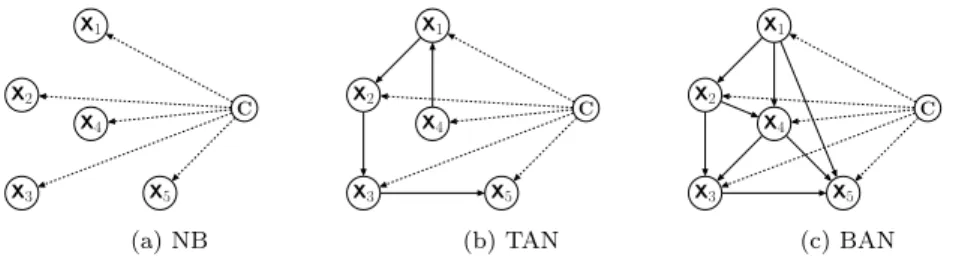
Na¨ıve Bayes (NB) is a well-known Bayesian classifier which is very computa-tionally efficient and has in general good predictive performance. NB is based on the assumption that features are independent from each other, given the class variable. An example network topology is shown in Figure 1(a), where the edges indicate that each feature depends only on the class (their only par-ent node). To classify a testing instance, NB computes the probability of each class label c given all the feature values (x1, x2,..., xm) of the instance

us-ing Equation (1) and assigns the instance to the class label with the greatest probability.

P

(

c

|

x

1

, x

2

, ..., x

m

)

∝

P

(

c

)

m

Q

i=1

P

(

x

_i

|

c

)

(1)

In Equation (1),mis the number of features, and the probability of a class label c given all feature values of an instance is estimated by calculating the product of the prior probability ofctimes the probability of each feature value

xigiven c, using the above mentioned independence assumption.

2.2 Tree Augmented Na¨ıve Bayes (TAN) Classifier

TAN is a type of semi-Na¨ıve Bayes classifier that relaxes Na¨ıve Bayes’ feature independence assumption, by allowing each feature to depend on at most one other feature (in addition to depending on the class, which is a parent node of all features). An example network topology is shown in Figure 1(b), where all nodes except X4 have one non-class variable parent node. This increases the ability to represent feature dependencies (which may lead to improved predictive accuracy) and still leads to reasonably efficient algorithms. TAN algorithms are not as efficient (fast) as NB, but TAN algorithms are in general much more efficient and scalable than other Bayesian classification algorithms that allow a feature to depend on several features. Among the several types of TAN algorithms, e.g., in (Friedman et al 1997; Keogh and Pazzani 1999; Jiang et al 2005; Zhang and Ling 2001), in this work we focus on one of the most

(6)

computationally efficient ones, which is based on the principle of maximizing the conditional mutual information (CMI) for each pair of features given the class attribute (Friedman et al 1997). Then, the Maximum Weight Spanning Tree (MST) will be built, where the weight of an edge is given by its CMI. Finally, one vertex of the MST is randomly selected as the root, and the edge directions are propagated accordingly.

2.3 Bayesian Network Augmented Na¨ıve Bayes (BAN) Classifier

Comparing with Na¨ıve Bayes and TAN classifiers, a Bayesian Network Aug-mented Na¨ıve Bayes (BAN) classifier is a type of more sophisticated semi-Na¨ıve Bayes classifier that allows each feature to have more than one parents. An example network topology is shown in Figure 1(c), where node X4 has two parent nodes, i.e., X1and X2. The conventional algorithm to construct a BAN is analogous to the one for learning the TAN classifier (Friedman et al 1997). In this work, instead of learning the feature dependencies by conventional meth-ods, we adopt the approach proposed in (Wan and Freitas 2013, 2015), where the network edges representing feature dependencies are simply the pre-defined edges in the feature hierarchy. More precisely, in (Wan and Freitas 2013, 2015), a classifier called GO–hierarchy–aware BAN (GO–BAN) directly adopted the edges of the Gene Ontology (GO)’s DAG (Directed Acyclic Graph) (The Gene Ontology Consortium 2000) – see Section 2.5 – as the topology of the BAN network. This has the advantages of saving computational time and exploiting the background knowledge associated with the Gene Ontology, which incor-porates the expertise of a large number of biologists.

X1 X2 X3 X5 X4 C (a) NB X1 X2 X3 X5 X4 C (b) TAN X1 X2 X3 X5 X4 C (c) BAN Fig. 1: Topology of Different Bayesian Network Classifiers

2.4 Lazy Learning

A “lazy” learning method performs the learning process in the testing phase, building a specific classification model for each new testing instance to be classified (Aha 1997; Pereira et al 2011). This is in contrast to the usual “eager” learning approach, where a classification model is learnt from the training

(7)

instances before any testing instance is observed. In the context of feature selection, lazy learning selects a specific set of features for each individual testing instance, whilst eager learning selects a single set of features for all testing instances. The hierarchical feature selection methods evaluated in this work are lazy methods, because they exploit hierarchical information which is specific to each instance, in order to select the best set of features for each instance – as described later. Hence, we also use lazy versions of NB, TAN and GO–BAN in our experiments.

2.5 The Gene Ontology and Hierarchical Feature Redundancy

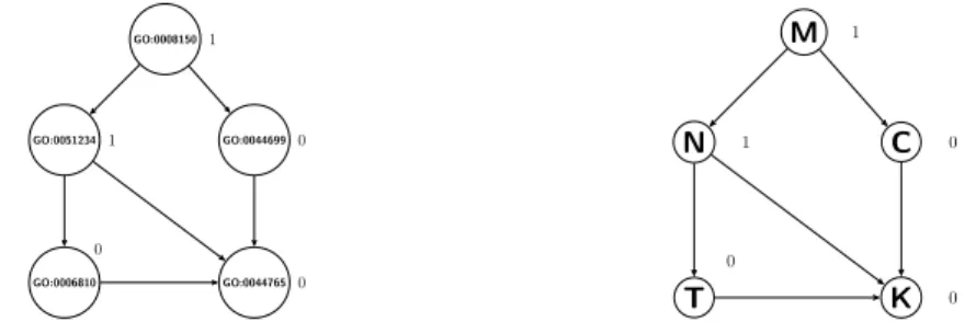
The Gene Ontology (GO) uses unified and structured vocabularies to describe gene functions (The Gene Ontology Consortium 2000). There are three types of GO terms: biological process, molecular function and cellular component. Most GO terms are hierarchically structured by an “is-a” relationship, where each GO term is a specialization of its ancestor (more generic) terms. There-fore, there are three DAGs representing the three types of GO terms. For ex-ample, as shown in Figure 2(a), GO:0008150 (biological process) is the root of the DAG for biological process terms, and it is also the parent of GO:0051234 (establishment of localization), which is in turn the parent of GO:0006810 (transport). GO:0008150 GO:0051234 GO:0006810 GO:0044699 GO:0044765 1 1 0 0 0

(a) A small part of the Gene Ontology’s topology

M N T C K 1 1 0 0 0

(b) Example of Hierarchical Redundancy Fig. 2: Example of Hierarchically Structured Features

Consider a hierarchy of features, where each feature represents a GO term which is a node in a GO DAG. Each feature takes a binary value, “1” or “0”, indicating whether or not an instance (a gene) is annotated with the corresponding GO term. The “is-a” hierarchy of the GO is associated with two hierarchical constraints. First, if a feature takes the value “1” for a given instance, this implies its ancestors in the DAG also take the value “1” for that instance. For example, in Figure 2(a), if the term GO:0051234 has value “1” for a given gene, then the value of term GO:0008150 should be “1” as well. Conversely, if the feature takes the value “0” for a given instance, this implies

(8)

that its descendants in the DAG also take the value “0” for that instance. For example, if the term GO:0006810 has value “0”, then term GO:0044765 should also have value “0”.

Hierarchical feature redundancy is defined in this work as the case where there are two or more nodes which have the same value (“1” or “0”) in an individual instance and are located in the same path from a root to a leaf node in the DAG. For instance, in Figure 2(b), where the number “1” or “0” beside a node is the value of that feature in a given instance, nodes N and M are redundant, since both have value “1” and are located in the same path, i.e., M–N–T–K or M–N–K. Analogously, nodes T and K are redundant, since both have value “0” and are in the same path M–N–T–K. Nodes C and K are also redundant, since both have value “0” and are in the path M–C–K. Removing this type of hierarchical feature redundancy is the core task performed by the hierarchical feature selection methods used in this work.

3 Hierarchical Feature Selection Methods – Select Hierarchical Information-Preserving (HIP) Features and Select Most Relevant (MR) Features

In our previous works (Wan and Freitas 2013; Wan et al 2015; Wan and Fre-itas 2015), we proposed three lazy learning-based hierarchical feature selec-tion methods to cope with the hierarchical feature redundancy issue discussed in Section 2.5. These methods are called Select Hierarchical Information-Preserving (HIP) features, Select Most Relevant (MR) features, and the hybrid HIP–MR method. In general, both HIP and MR select a set of features without hierarchical redundancy, whereas HIP–MR usually generates a set of features where the redundancy issue is only alleviated, but not eliminated (Wan et al 2015). Hence, both HIP and MR select much fewer features, and they obtained substantially greater predictive accuracy than the hybrid HIP–MR in the ex-periments reported in (Wan et al 2015). Hence, we use only HIP and MR in this work.

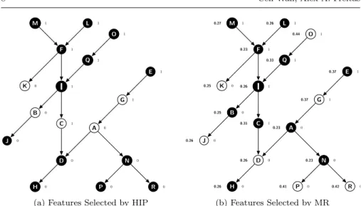
HIP and MR perform “lazy” feature selection, i.e., they select a specific set of features for each testing instance, based on the feature values observed in that instance. The HIP method selects only features whose values are not implied by the value of any other feature in the current testing instance, due to the hierarchical constraints (see Section 2.5). For instance, in Figure 3(a), the value of node (feature) C is not implied by any other feature’s value, but its value “1” implies that the values of its ancestors I, F, M, L, Q and O are also “1”; the value of node A is also not implied by any other feature’s value, but its value “0” implies that the values of nodes D, H, N, P and R are also “0”. HIP will select nodes K, B, C, A and G for the example DAG of Figure 3(a), since this feature subset preserves all the hierarchical information – i.e., for any given instance, the values of the features in this subset imply the values of all the other features.

(9)

F I C D K L B J H A G E M Q O N P R 1 1 0 1 0 0 1 0 0 0 1 1 1 1 1 0 0 0

(a) Features Selected by HIP

F I C D K L B J H A G E M Q O N P R 0.23 0.26 0.31 0.26 0.25 0.26 0.25 0.26 0.26 0.23 0.37 0.37 0.27 0.23 0.41 0.42 0.33 0.44 1 1 0 1 0 0 1 0 0 0 1 1 1 1 1 0 0 0 (b) Features Selected by MR Fig. 3: Example of Hierarchical Feature Selection by HIP and MR

The MR method selects the feature with maximal relevance value in the set of features whose values equal to “1” or “0” in each path of the feature DAG. If there exist more than one features having the maximal relevance value, only the deepest (most specific) one (if the feature value is “1”) or the shallowest (most generic) one (if the feature value is “0”) in that path will be selected. Equation 2 is used to measure the relevance (R) (predictive power) of a binary feature X, which can take valuex1orx2. In this equation,n denotes the number of classes andcidenotes thei-th class label. Equation 2 measures

R(X) =

n

X

i=1

[P(ci|x1)−P(ci|x2)]2 (2)

the relevance of a feature as a function of the difference in the conditional probabilities of each class given different values (“1” or “0”) of the feature. In the example DAG in Figure 3(b), where the numbers on the left side of nodes denote the corresponding relevance values and and the numbers on the right side of nodes denote the binary feature values, the MR method selects 7 nodes, namely K, J, D, P, R, G and O. In detail, MR selects node O rather than node Q, since the former has higher relevance value and both nodes have the value “1” in the same path; and it selects node G rather than node E, since the former is deeper than the latter and both nodes have value “1” in the same path. Analogously, MR selects node J rather than node B, since the former has higher relevance value and both nodes have the value “0” in the same path; and it selects node D rather than node H, since the former is shal-lower and both nodes have value “0” in the same path. Note that, in this case, the features selected by MR will lead to some hierarchical information loss. For example, the value “1” of selected node O does not imply that the value of non-selected node Q is also “1”, and the Q’s value is not implied by the

(10)

value of any selected node (so the information that Q has value “1” was lost). Similarly, the value “0” of selected node J does not imply that non-selected node B has value “0”, and B’s value is not implied by the value of any selected node.

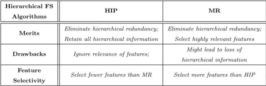
As summarized in Table 1, both HIP and MR have the merit of elimi-nating hierarchical feature redundancy. However, they differ in other aspects, with their own merits and drawbacks, i.e., HIP selects features retaining all hierarchical information whilst ignoring the relevance of features with the class attribute; whereas MR selects features having higher relevance to the class at-tribute, but the selected features might not retain the complete hierarchical information (i.e., leading to loss of hierarchical information).

Table 1: Summary of Characteristics of the HIP and MR Methods

Hierarchical FS

HIP MR

Algorithms

Merits Eliminate hierarchical redundancy; Eliminate hierarchical redundancy; Retain all hierarchical information Select highly relevant features Drawbacks Ignore relevance of features; Might lead to loss of

hierarchical information Feature

Select fewer features than MR Select more features than HIP Selectivity

4 Experimental Methodology and Computational Results 4.1 Dataset Creation

We constructed 28 datasets with data about the effect of genes on an organ-ism’s longevity, by integrating data from the Human Ageing Genomic Re-sources (HAGR) GenAge database (Build 17) (de Magalh˜aes et al 2009) and the Gene Ontology (GO) database (version: 2014-06-13) (The Gene Ontol-ogy Consortium 2000). HAGR provides longevity-related gene data for four model organisms, i.e.,C. elegans (worm),D. melanogaster (fly),M. musculus (mouse) and S. cerevisiae (yeast). For details of the dataset creation proce-dure, see (Wan and Freitas 2013; Wan et al 2015). However, in (Wan and Freitas 2013; Wan et al 2015) we created datasets using only Biological Pro-cess GO terms; whilst in this current work we created datasets with all three types of GO terms, each type associated with a hierarchy (see Section 2.5) in the form of a DAG: Biological Process (BP), Molecular Function (MF) and Cellular Component (CC) GO terms. Note that the different types of GO terms are contained in DAGs whose sets of nodes do not intersect with each other. This means that the hierarchical feature selection methods conduct the feature selection process based on each individual DAG separately.

(11)

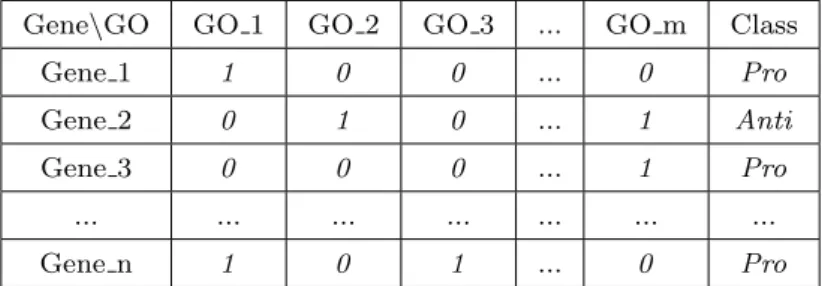
In the created datasets, the instances represent aging-related genes, the fea-tures represent hierarchical GO terms, and the class variable indicates whether the gene contributes to increasing or decreasing the longevity of an organism. For each model organism, we created 7 datasets, with all possible subsets of the three GO term types, i.e., one dataset for each GO term type (BP, MF, CC), one dataset for each pair of GO term types (BP and MF, BP and CC, MF and CC), and one dataset with all 3 GO term types (BP, MF and CC). The struc-ture of each created dataset is shown in Figure 4, where the feastruc-ture value “1” or “0” indicates whether or not (respectively) a GO term is annotated for each gene. In the class variable, the values “Pro” and “Anti” mean “pro-longevity” and “anti-longevity”. Pro-longevity genes are those whose decreased expression (due to knock–out, mutations or RNA interference) reduces lifespan and/or whose overexpression extends lifespan. Anti-longevity genes are those whose decreased expression extends lifespan and/or whose overexpression decreases lifespan (Tacutu et al 2013). Gene\GO GO 1 GO 2 GO 3 ... GO m Class Gene 1 1 0 0 ... 0 Pro Gene 2 0 1 0 ... 1 Anti Gene 3 0 0 0 ... 1 Pro ... ... ... ... ... ... ... Gene n 1 0 1 ... 0 Pro

Fig. 4: Structure of the Created Datasets

Note that GO terms with only one associated gene would be useless for building a classification model because they are extremely specific to an indi-vidual gene, and a model that includes these GO terms would be over-fitting the data. However, GO terms associated with only a few genes might be valu-able for discovering biological knowledge, since they might represent specific biological information. In our previous work (Wan et al 2015), we did experi-ments with different values of a threshold defining the minimum frequency of occurrence of a GO term which is required in order to include that term (as a feature) in a dataset, in order to perform effective classification. Based on that work, the threshold value of at least 3 occurrences is used here, which retains more biological information than higher thresholds while still leading to high predictive accuracy. In addition, the root GO terms – i.e., GO:0008150, GO:0003674 and GO:0005575, respectively for the DAG of biological process, molecular function and cellular component terms – are not included in the corresponding datasets, since the root GO terms have no predictive power (all genes are trivially annotated with each root GO term).

(12)

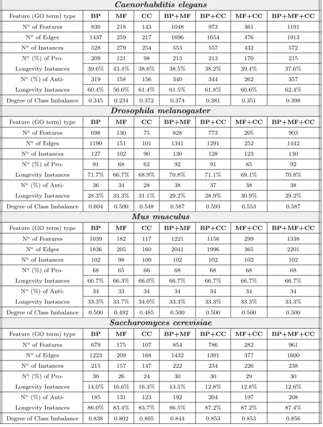
The main characteristics of the created datasets are shown in Table 2, which reports the number of features and edges in the GO DAG, the total number of instances, the number (and percentage) of instances in each class, and the degree of class imbalance. The degree of class imbalance is calculated by Equation 3, where the degree (D) equals to the complement of the ratio of the number of instances belonging to the minority class (No₍_{M inor}_{)) over} the number of instances belonging to the majority class (No₍_{M ajor}_)).

D= 1−N

o₍_{M inor}₎

No₍_{M ajor}₎ (3)

4.2 Experimental Methodology and Predictive Accuracy Measure

We evaluate two hierarchical feature selection methods – namely HIP and MR – and, as a baseline, the flat feature selection method CFS (Correlation-based Feature Selection). CFS is a well-known eager learning method that selects the same feature subset to classify all testing instances – instead of perform-ing lazy feature selection for each testperform-ing instance, like HIP and MR. CFS tries to select a feature subset where each feature has a high correlation with the class variable and the features have a low correlation with each other (to avoid selecting redundant features). Hence, CFS is an interesting baseline method because it tries to remove redundant features in a “flat” sense, without ex-ploiting the notion of hierarchically redundant features that is at the core of HIP and MR.

We perform three sets of experiments, using NB, TAN and GO–BAN as classifiers. The well-known 10-fold cross validation procedure was adopted to evaluate the predictive performance of NB, TAN and GO–BAN with different feature selection methods. The Geometric Mean (GMean) of the Sensitivity (Sen.) and Specificity (Spe.) is used to measure predictive accuracy, since the distributions of classes in the datasets are imbalanced. As shown in Equation 4, GMean is defined as the square root of the product ofSen.and Spe.; Sen. denotes the percentage of positive (“pro-longevity”) instances that are cor-rectly classified as positive, whereas Spe. denotes the percentage of negative (“anti-longevity”) instances that are correctly classified as negative.

GM ean=pSen.×Spe. (4)

4.3 Experimental Results

4.3.1 Feature selection results separately for each Bayesian classifier

Tables 3, 4 and 5 report the feature selection results separately for each type of Bayesian network classifier, namely Na¨ıve Bayes, TAN and BAN respectively. These tables have the same structure, reporting the results for 3 different

(13)

Table 2: Main Characteristics of the Created Datasets

Caenorhabditis elegans

Feature (GO term) type BP MF CC BP+MF BP+CC MF+CC BP+MF+CC

No_{of Features} ₈₃₀ ₂₁₈ ₁₄₃ ₁₀₄₈ ₉₇₃ ₃₆₁ ₁₁₉₁ No_{of Edges} ₁₄₃₇ ₂₅₉ ₂₁₇ ₁₆₉₆ ₁₆₅₄ ₄₇₆ ₁₉₁₃ No_{of Instances} ₅₂₈ ₂₇₉ ₂₅₄ ₅₅₃ ₅₅₇ ₄₃₂ ₅₇₂ No_{(%) of Pro-} ₂₀₉ ₁₂₁ ₉₈ ₂₁₃ ₂₁₃ ₁₇₀ ₂₁₅ Longevity Instances 39.6% 43.4% 38.6% 38.5% 38.2% 39.4% 37.6% No_{(%) of Anti-} ₃₁₉ ₁₅₈ ₁₅₆ ₃₄₀ ₃₄₄ ₂₆₂ ₃₅₇ Longevity Instances 60.4% 56.6% 61.4% 61.5% 61.8% 60.6% 62.4%

Degree of Class Imbalance 0.345 0.234 0.372 0.374 0.381 0.351 0.398

Drosophila melanogaster

No_{of Features} ₆₉₈ ₁₃₀ ₇₅ ₈₂₈ ₇₇₃ ₂₀₅ ₉₀₃ Noof Edges 1190 151 101 1341 1291 252 1442 No_{of Instances} ₁₂₇ ₁₀₂ ₉₀ ₁₃₀ ₁₂₈ ₁₂₃ ₁₃₀ No_{(%) of Pro-} ₉₁ ₆₈ ₆₂ ₉₂ ₉₁ ₈₅ ₉₂ Longevity Instances 71.7% 66.7% 68.9% 70.8% 71.1% 69.1% 70.8% No_{(%) of Anti-} ₃₆ ₃₄ ₂₈ ₃₈ ₃₇ ₃₈ ₃₈ Longevity Instances 28.3% 33.3% 31.1% 29.2% 28.9% 30.9% 29.2%

Mus musculus

No_{of Features} ₁₀₃₉ ₁₈₂ ₁₁₇ ₁₂₂₁ ₁₁₅₆ ₂₉₉ ₁₃₃₈ No_{of Edges} ₁₈₃₆ ₂₀₅ ₁₆₀ ₂₀₄₁ ₁₉₉₆ ₃₆₅ ₂₂₀₁ No_{of Instances} ₁₀₂ ₉₈ ₁₀₀ ₁₀₂ ₁₀₂ ₁₀₂ ₁₀₂ No_{(%) of Pro-} ₆₈ ₆₅ ₆₆ ₆₈ ₆₈ ₆₈ ₆₈ Longevity Instances 66.7% 66.3% 66.0% 66.7% 66.7% 66.7% 66.7% No(%) of Anti- 34 33 34 34 34 34 34 Longevity Instances 33.3% 33.7% 34.0% 33.3% 33.3% 33.3% 33.3%

Saccharomyces cerevisiae

Noof Features 679 175 107 854 786 282 961 No_{of Edges} ₁₂₂₃ ₂₀₉ ₁₆₈ ₁₄₃₂ ₁₃₉₁ ₃₇₇ ₁₆₀₀ No_{of Instances} ₂₁₅ ₁₅₇ ₁₄₇ ₂₂₂ ₂₃₄ ₂₂₆ ₂₃₈ No_{(%) of Pro-} ₃₀ ₂₆ ₂₄ ₃₀ ₃₀ ₂₉ ₃₀ Longevity Instances 14.0% 16.6% 16.3% 13.5% 12.8% 12.8% 12.6% No_{(%) of Anti-} ₁₈₅ ₁₃₁ ₁₂₃ ₁₉₂ ₂₀₄ ₁₉₇ ₂₀₈ Longevity Instances 86.0% 83.4% 83.7% 86.5% 87.2% 87.2% 87.4%

(14)

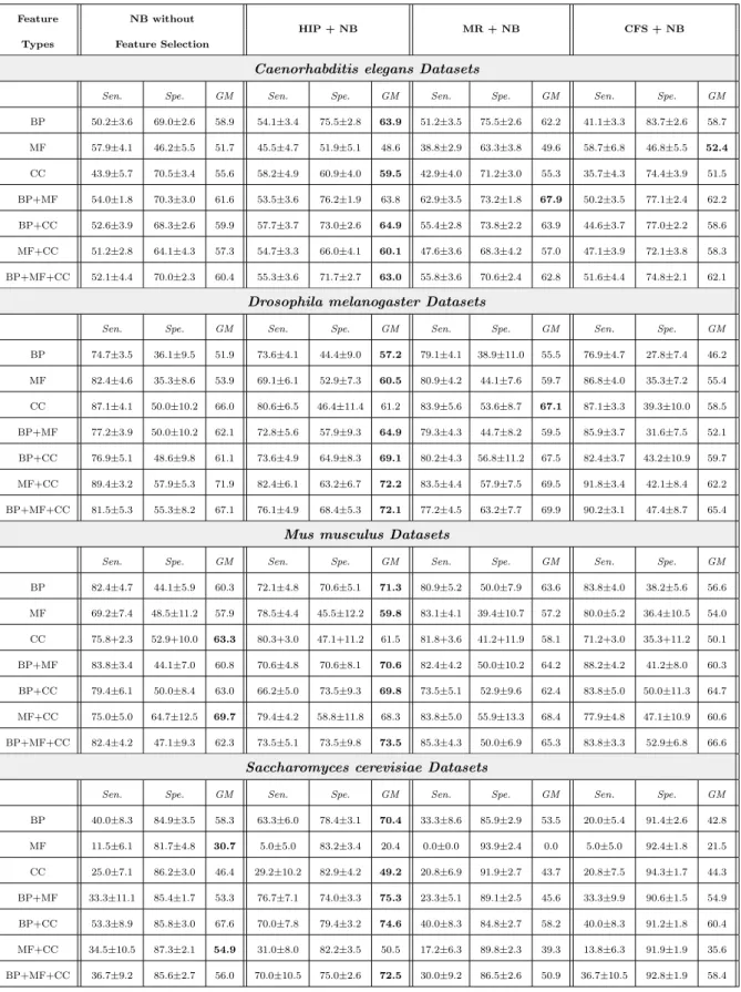
Table 3: Predictive Accuracy (%) for Na¨ıve Bayes with Hierarchical Feature Selection Methods HIP, MR and “Flat” Feature Selection Method CFS

Feature NB without

HIP + NB MR + NB CFS + NB

Types Feature Selection

Caenorhabditis elegans Datasets

Sen. Spe. GM Sen. Spe. GM Sen. Spe. GM Sen. Spe. GM

BP 50.2±3.6 69.0±2.6 58.9 54.1±3.4 75.5±2.8 63.9 51.2±3.5 75.5±2.6 62.2 41.1±3.3 83.7±2.6 58.7 MF 57.9±4.1 46.2±5.5 51.7 45.5±4.7 51.9±5.1 48.6 38.8±2.9 63.3±3.8 49.6 58.7±6.8 46.8±5.5 52.4 CC 43.9±5.7 70.5±3.4 55.6 58.2±4.9 60.9±4.0 59.5 42.9±4.0 71.2±3.0 55.3 35.7±4.3 74.4±3.9 51.5 BP+MF 54.0±1.8 70.3±3.0 61.6 53.5±3.6 76.2±1.9 63.8 62.9±3.5 73.2±1.8 67.9 50.2±3.5 77.1±2.4 62.2 BP+CC 52.6±3.9 68.3±2.6 59.9 57.7±3.7 73.0±2.6 64.9 55.4±2.8 73.8±2.2 63.9 44.6±3.7 77.0±2.2 58.6 MF+CC 51.2±2.8 64.1±4.3 57.3 54.7±3.3 66.0±4.1 60.1 47.6±3.6 68.3±4.2 57.0 47.1±3.9 72.1±3.8 58.3 BP+MF+CC 52.1±4.4 70.0±2.3 60.4 55.3±3.6 71.7±2.7 63.0 55.8±3.6 70.6±2.4 62.8 51.6±4.4 74.8±2.1 62.1

Drosophila melanogaster Datasets

Mus musculus Datasets

BP 82.4±4.7 44.1±5.9 60.3 72.1±4.8 70.6±5.1 71.3 80.9±5.2 50.0±7.9 63.6 83.8±4.0 38.2±5.6 56.6 MF 69.2±7.4 48.5±11.2 57.9 78.5±4.4 45.5±12.2 59.8 83.1±4.1 39.4±10.7 57.2 80.0±5.2 36.4±10.5 54.0 CC 75.8+2.3 52.9+10.0 63.3 80.3+3.0 47.1+11.2 61.5 81.8+3.6 41.2+11.9 58.1 71.2+3.0 35.3+11.2 50.1 BP+MF 83.8±3.4 44.1±7.0 60.8 70.6±4.8 70.6±8.1 70.6 82.4±4.2 50.0±10.2 64.2 88.2±4.2 41.2±8.0 60.3 BP+CC 79.4±6.1 50.0±8.4 63.0 66.2±5.0 73.5±9.3 69.8 73.5±5.1 52.9±9.6 62.4 83.8±5.0 50.0±11.3 64.7 MF+CC 75.0±5.0 64.7±12.5 69.7 79.4±4.2 58.8±11.8 68.3 83.8±5.0 55.9±13.3 68.4 77.9±4.8 47.1±10.9 60.6 BP+MF+CC 82.4±4.2 47.1±9.3 62.3 73.5±5.1 73.5±9.8 73.5 85.3±4.3 50.0±6.9 65.3 83.8±3.3 52.9±6.8 66.6

Saccharomyces cerevisiae Datasets

(15)

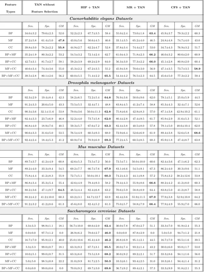
Table 4: Predictive Accuracy (%) for TAN with Hierarchical Feature Selection Methods HIP, MR and “Flat” Feature Selection Method CFS

Feature TAN without

HIP + TAN MR + TAN CFS + TAN

Caenorhabditis elegans Datasets

BP 34.0±3.2 79.6±2.3 52.0 52.2±2.3 67.7±3.5 59.4 55.0±2.4 73.0±1.8 63.4 45.9±3.7 79.3±2.2 60.3 MF 37.2±5.8 61.4±5.0 47.8 43.0±5.6 50.6±4.5 46.6 33.1±3.5 65.2±4.0 46.5 24.8±4.8 74.7±4.0 43.0 CC 39.8±3.0 78.2±2.2 55.8 44.9±2.7 62.2±4.7 52.8 37.8±3.4 74.4±2.7 53.0 34.7±4.3 76.9±3.2 51.7 BP+MF 35.2±1.9 80.3±2.2 53.2 54.5±3.2 72.1±2.4 62.7 61.0±4.3 71.8±2.3 66.2 46.0±3.2 80.6±2.0 60.9 BP+CC 42.7±3.1 81.7±2.7 59.1 59.2±3.9 69.2±2.9 64.0 56.3±3.0 77.3±2.2 66.0 45.1±2.8 80.8±2.0 60.4 MF+CC 40.6±3.4 74.4±3.6 55.0 45.3±2.2 67.2±3.5 55.2 45.9±3.8 70.6±3.0 56.9 47.1±3.5 73.7±3.5 58.9 BP+MF+CC 39.5±2.8 80.1±2.6 56.2 60.0±5.5 71.4±2.2 65.5 54.4±4.2 76.5±2.3 64.5 45.6±5.0 77.3±2.2 59.4 Drosophila melanogaster Datasets

BP 92.3±2.9 19.4±8.4 42.3 58.2±6.5 72.2±5.4 64.8 76.9±3.6 50.0±9.6 62.0 79.1±5.1 25.0±5.9 44.5 MF 91.2±3.3 20.6±5.0 43.3 73.5±5.5 32.4±7.1 48.8 83.8±4.5 41.2±7.4 58.8 85.3±4.3 32.4±7.1 52.6 CC 90.3±3.6 32.1±11.6 53.8 79.0±3.6 50.0±11.3 62.8 75.8±6.6 42.9±8.3 57.0 87.1±3.8 42.9±10.2 61.1 BP+MF 92.4±3.3 23.7±6.9 46.8 52.2±4.0 73.7±5.8 62.0 80.4±2.8 47.4±9.5 61.7 85.9±2.9 31.6±5.3 52.1 BP+CC 86.8±4.0 18.9±7.6 40.5 59.3±5.7 67.6±7.2 63.3 82.4±3.8 40.5±8.0 57.8 79.1±5.0 48.6±10.4 62.0 MF+CC 90.6±3.3 31.6±5.0 53.5 76.5±4.9 60.5±9.3 68.0 72.9±6.4 52.6±6.9 61.9 89.4±3.8 52.6±5.8 68.6 BP+MF+CC 92.4±2.4 18.4±5.3 41.2 60.9±7.6 78.9±6.9 69.3 77.2±4.5 60.5±8.5 68.3 85.9±1.8 47.4±8.7 63.8 Mus musculus Datasets

Saccharomyces cerevisiae Datasets

(16)

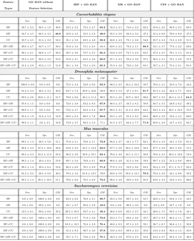
Table 5: Predictive Accuracy (%) for GO–BAN with Hierarchical Feature Se-lection Methods HIP, MR and “Flat” Feature SeSe-lection Method CFS

Feature GO–BAN without

HIP + GO–BAN MR + GO–BAN CFS + GO–BAN

Caenorhabditis elegans

BP 28.7±2.2 86.5±1.8 49.8 54.5±3.2 73.4±2.7 63.2 52.2±3.1 74.0±2.2 62.2 45.0±2.6 80.9±2.5 60.3 MF 34.7±4.5 66.5±4.5 48.0 43.8±4.5 52.5±5.2 48.0 35.5±3.0 63.3±3.4 47.4 31.4±6.6 70.9±6.0 47.2 CC 33.7±4.5 81.4±2.2 52.4 55.1±5.0 63.5±4.0 59.2 40.8±4.3 73.1±2.6 54.6 35.7±4.3 74.4±3.9 51.5 BP+MF 30.0±2.7 84.7±1.7 50.4 55.9±3.2 74.1±2.5 64.4 63.8±2.2 73.2±2.1 68.3 52.1±3.7 77.6±2.2 63.6 BP+CC 29.1±2.1 86.6±1.7 50.2 58.7±3.6 72.7±2.5 65.3 54.0±2.8 74.7±2.3 63.5 47.4±2.7 79.1±1.5 61.2 MF+CC 35.3±2.9 80.2±3.2 53.2 55.9±3.1 64.5±3.6 60.0 47.1±3.4 70.2±3.9 57.5 46.5±4.1 72.1±4.0 57.9 BP+MF+CC 31.2±2.9 85.2±1.5 51.6 58.1±3.8 73.4±2.6 65.3 55.3±4.0 72.0±2.6 63.1 50.7±4.1 75.4±2.1 61.8 Drosophila melanogaster

BP 100.0±0.0 0.0±0.0 0.0 75.8±4.4 52.8±8.6 63.3 80.2±3.5 44.4±10.2 59.7 78.0±4.1 25.0±7.8 44.2 MF 91.2±3.3 26.5±3.4 49.2 64.7±7.2 50.0±10.0 56.9 80.9±5.2 47.1±9.1 61.7 85.3±4.3 32.4±7.1 52.6 CC 93.5±2.6 28.6±11.1 51.7 79.0±6.6 46.4±11.4 60.5 85.5±4.6 42.9±10.2 60.6 88.7±3.5 46.4±11.4 64.2 BP+MF 97.8±1.5 0.0±0.0 0.0 72.8±3.9 63.2±9.3 67.8 80.4±3.7 44.7±8.2 59.9 83.7±3.5 28.9±6.2 49.2 BP+CC 98.9±1.1 0.0±0.0 0.0 73.6±4.7 62.2±8.4 67.7 80.2±4.1 51.4±10.9 64.2 82.4±4.4 40.5±10.2 57.8 MF+CC 95.3±1.9 31.6±5.3 54.9 80.0±6.2 60.5±7.6 69.6 83.5±4.9 55.3±8.2 68.0 90.6±3.0 52.6±4.5 69.0 BP+MF+CC 98.9±1.1 2.6±2.5 16.0 73.9±4.7 68.4±5.3 71.1 81.5±3.7 63.2±7.7 71.8 88.0±2.6 44.7±8.2 62.7 Mus musculus

BP 98.5±1.4 26.5±5.0 51.1 75.0±5.1 70.6±5.1 72.8 88.2±4.7 44.1±7.7 62.4 85.3±4.3 44.1±5.9 61.3 MF 90.8±3.3 27.3±10.0 49.8 84.6±3.0 45.5±12.2 62.0 87.7±3.0 39.4±10.6 58.8 87.7±2.9 30.3±9.6 51.5 CC 86.4±3.3 35.3±11.2 55.2 80.3±3.0 50.0±10.1 63.4 78.8±3.8 44.1±11.1 58.9 78.8±3.3 38.2±12.6 54.9 BP+MF 98.5±1.4 29.4±6.4 53.8 69.1±5.8 70.6±8.1 69.8 86.8±4.0 41.2±9.6 59.8 89.7±2.2 41.2±8.0 60.8 BP+CC 98.5±1.4 29.4±6.4 53.8 66.2±6.0 76.5±8.0 71.2 77.9±5.3 52.9±9.6 64.2 82.4±5.6 47.1±11.7 62.3 MF+CC 91.2±3.2 26.5±8.8 49.2 79.4±4.2 61.8±12.5 70.0 83.8±5.0 58.8±13.1 70.2 79.4±4.8 44.1±9.6 59.2 BP+MF+CC 98.5±1.4 26.5±10.5 51.1 70.6±6.0 76.5±8.8 73.5 86.8±4.0 50.0±6.9 65.9 83.8±3.3 52.9±8.4 66.6 Saccharomyces cerevisiae

(17)

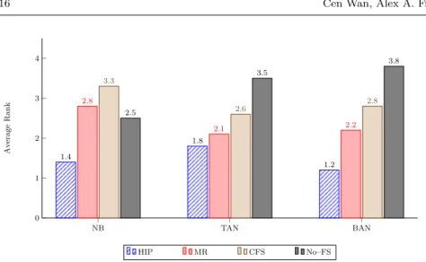
NB TAN BAN 0 1 2 3 4 1.4 1.8 1.2 2.8 2.1 2.2 3.3 2.6 2.8 2.5 3.5 3.8 Av era ge Rank HIP MR CFS No–FS

Fig. 5: Average Ranks for Feature Selection Methods with Different Classifiers

feature selection methods in a pre-processing phase, namely two hierarchi-cal feature selection methods, HIP and MR, and the “flat” feature selection method CFS, and also when not using any feature selection method. Each ta-ble contains the results for 28 datasets – 7 combinations of feature (GO term) types for each of 4 model organisms. For each of the 28 datasets in each table, we compute a ranking of the feature selection methods, where ranks 1 and 4 represent the best and worst GMean values, respectively, in that dataset. The average rank (across the 28 datasets) is then shown in Figure 5, which summarizes the results of Tables 3–5.

Table 3 compares the predictive accuracies obtained by Na¨ıve Bayes. As shown in the group of bars in the left side of Figure 5, the HIP method ob-tains the best average rank of 1.4. The second, third and worst results were obtained by Na¨ıve Bayes without feature selection (No–FS), MR and CFS, with average ranks of 2.5, 2.8 and 3.3, respectively. It is obvious that HIP performs best when it works with Na¨ıve Bayes, since it is ranked in the first position (indicated by a GMean value in boldface font in Table 3) in 21 out of the 28 datasets.

Table 4 compares the predictive accuracies obtained by TAN. As shown in the group of bars in the middle of Figure 5, the HIP method again obtained the best average rank (1.8), and it ranked first in 15 out of the 28 datasets in Table 4. MR obtained the second best average rank (2.1). The third and worst results were obtained by CFS and TAN without feature selection (No–FS), with average ranks of 2.6 and 3.5, respectively.

Table 5 compares the predictive accuracies obtained by GO–BAN. As shown in the group of bars in the right side of Figure 5, the HIP method again obtained the best average rank (1.2), and it ranked first in 23 out of the 28 datasets in Table 5. MR obtained the second best average rank (2.2). The third and worst results were obtained by CFS and GO–BAN without feature

(18)

selection (No–FS), with average ranks of 2.8 and 3.8, respectively.

4.3.2 Global comparison of feature selection methods combined with three different types of Bayesian classifiers

This section considers each pair of a feature selection approach combined with a type of Bayesian network classifier as a whole “classification approach”, and compares the predictive performance of the 12 classification approaches used in our experiments, rather than evaluating the results of each feature selection method separately for each type of Bayesian classifier like in the previous section. Note that we have 12 classification approaches because there are 4 feature selection approaches (3 feature selection methods and the no feature selection approach) and 3 Bayesian classifiers. Figure 6 shows the average rank (based on Gmean values) for each classification approach, across the 28 datasets. Table 6 shows the number of wins (where the highest GMean value was obtained) by each classification approach.

0 2 4 6 8 10 12 No–FS+GO–BAN No–FS+TAN CFS+TAN CFS+GO–BAN CFS+NB MR+TAN MR+NB HIP+TAN No–FS+NB MR+GO–BAN HIP+NB HIP+GO–BAN 11.3 9.8 9.2 7.8 7.1 6.1 5.6 5.5 5.4 5.4 2.5 2.4 Average Rank

Fig. 6: Ranking of the 12 classification approaches (each combining a feature selection approach with a type of Bayesian classifier)

HIP+GO–BAN achieved the best average rank, 2.4 (Figure 6), and the second highest number of wins, 7 (Table 6). HIP+NB achieved the second best rank (2.5), and the highest number of wins, 11. Clearly both HIP+GO–BAN and HIP+NB obtained substantially better results (particularly in terms of

(19)

average rank, as shown in Figure 6 than the other classification approaches. In general, classification approaches using MR obtained better average ranks than classification approaches using CFS in Figure 6. The two worst classification approaches in that Figure involved no feature selection. In addition, as shown in Table 6, HIP and MR obtained in total 22 and 6 wins, respectively. By contrast, both CFS and the no feature selection approach did not win in any dataset, as shown in Table 6.

Table 6: Number of Wins (Best Gmean Values) Obtained by Each Combina-tion of a Feature SelecCombina-tion Approach and a Bayesian Classifier

Feature

HIP MR CFS No–FS

Selection Methods Bayesian

NB TAN BAN NB TAN BAN NB TAN BAN NB TAN BAN

Classifiers

Wins 11 4 7 2 1 3 0 0 0 0 0 0

Σ(Wins) 22 6 0 0

5 Discussion

5.1 Results of Statistical Significance Tests on Predictive Accuracy

We adopted the Friedman test and Holmpost-hocmethod to conduct a signifi-cance test on the differences between the GMean values of the feature selection methods, when using NB, TAN and GO–BAN as classifiers. The Friedman test is a non-parametric statistical test based on the ranks of each classifier’s GMean value on each dataset (Japkowicz and Shah 2011; Derrac et al 2011). The Holm post-hoc method is used for coping with the multiple-comparison problem when using significance tests, by adjusting the significance level for pairwise method comparisons (Demsˇar 2006).

We firstly conducted the significance test on different feature selection methods working with each of the different Bayesian classifiers. The signifi-cance tests results are shown in Table 7, where the feature selection methods’ average ranks are shown in columns 2, 6 and 10 for those methods working with NB, TAN and GO–BAN, respectively. Recall that a lower rank value means a better predictive performance. Columns 3, 7 and 11 show the p-value result of the significance test for each feature selection method compared with the best (control) method, and columns 4, 8 and 12 show the significance level adjusted by the Holmpost-hoc method. The difference between the ranks of two meth-ods is deemed statistically significant when the p-value is smaller than the corresponding adjusted significance level, which is indicated by a p-value in boldface font. HIP (the best method, used as the control method when working with either NB, TAN and GO–BAN) is compared with the other feature selec-tion methods and with not using any feature selecselec-tion method (row “No–FS”).

(20)

Table 7: Statistical Test Results of the Algorithms’ GMean Values According to the Non-parametric Friedman Test with the HolmPost-hoc Test at theα

= 0.05 Significance Level – results for experiments in Section 4.3.1

NB TAN GO–BAN

FS Method Ave. Rank P-Value Adjustedα FS Method Ave. Rank P-Value Adjustedα FS Method Ave. Rank P-Value Adjustedα

HIP (ctrl.) 1.4 – – HIP (ctrl.) 1.8 – – HIP (ctrl.) 1.2 – –

No–FS 2.5 1.4 E-03 0.0500 MR 2.1 3.8 E-01 0.0500 MR 2.2 3.7 E-03 0.0500

MR 2.8 4.9 E-05 0.0250 CFS 2.6 2.0 E-02 0.0250 CFS 2.8 3.5 E-06 0.0250

CFS 3.3 3.6 E-08 0.0167 No–FS 3.5 8.3 E-07 0.0167 No–FS 3.8 4.9 E-14 0.0167

Table 8: Statistical Test Results of the Algorithms’ GMean Values According to the Non-parametric Friedman Test with the HolmPost-hoc Test at theα

= 0.05 Significance Level – results for experiments in Section 4.3.2

FS Method Ave. Rank P-Value Adjustedα

HIP+GO–BAN (ctrl.) 2.4 – –

HIP+NB 2.5 9.17 E-1 5.00 E-2

MR+GO–BAN 5.4 1.85 E-3 2.50 E-2

No–FS+NB 5.4 1.85 E-3 1.67 E-2

HIP+TAN 5.5 1.30 E-3 1.25 E-2

MR+NB 5.6 0.90 E-4 1.00 E-2

MR+TAN 6.1 1.23 E-4 8.30 E-3

CFS+NB 7.1 1.08 E-6 7.10 E-3

CFS+GO–BAN 7.8 2.09 E-8 6.30 E-3

CFS+TAN 9.2 1.70 E-12 5.60 E-3

No–FS+TAN 9.8 1.60 E-14 5.00 E-3

No–FS+GO–BAN 11.3 2.56 E-20 4.60 E-3

The tests’ outcomes show that HIP significantly improves the performance of Na¨ıve Bayes without feature selection, and significantly outperforms the MR and CFS feature selection methods when using Na¨ıve Bayes. In addition, HIP significantly improves the performance of CFS when working with TAN, and significantly improves the predictive performance of TAN without feature se-lection, but it shows a non-significant difference with respect to MR using TAN. HIP also significantly outperforms MR and CFS when working with GO–BAN, and significantly improves the predictive performance of GO–BAN without feature selection.

(21)

We then conducted a significance test on the results comparing all 12 clas-sification approaches – each of which is a combination of a feature selection approach and a type of Bayesian classifier, as explained earlier. The results are shown in Table 8, where HIP+GO–BAN is ranked first and used as the control method. The results indicate that HIP+GO–BAN significantly outperforms all other compared methods, except HIP+NB.

5.2 Number of Features Selected by HIP, MR and CFS

Figure 7 shows the average number of features selected by HIP, MR and CFS methods for each of the 7 different types of datasets, each with a different set of GO term types. Each result is the average over the 4 model organisms. HIP consistently selected fewer features than MR, while CFS selects the smallest number of features among the three methods.

BP MF CC BP+MF BP+CC MF+CC BP+MF+CC 0 50 100 150 200 250 NO. of Selected F eatures HIP MR CFS

Fig. 7: Average number of features selected by HIP, MR or CFS for each of the feature (GO term) types – averaged over the 4 model organisms

5.3 Robustness of Predictive Performance Against Imbalanced Class Distributions

As shown in Figure 8, the degree of class imbalance (calculated by Equation 3) for the datasets range from 0.35, for the Caenorhabditis elegans datasets, to 0.84, for theSaccharomyces cerevisiae datasets.

We evaluated the HIP, MR and CFS methods from the perspective of robustness of predictive performance against large degrees of class imbalance, by computing the linear correlation coefficient (r) between the degree of class

(22)

C. elegans M. musculus D. melanogaster S.cerevisiae 0.4 0.6 0.8 0.35 0.5 0.57 0.84 Class Im balance

Fig. 8: Average degree of class imbalance for each of the 4 model organisms datasets – averaged over the 7 feature (GO term) types

Table 9: Correlation Coefficient between GMean and Degree of Class Imbal-ance for Different Feature Selection Methods with Different Classifiers

Classifier No Feature HIP MR CFS

Selection

NB -0.258 -0.035 -0.483 -0.461

TAN -0.801 0.088 -0.515 -0.406

GO–BAN -0.789 0.103 -0.463 -0.525

imbalance and GMean values over the 28 datasets. As shown in Table 9, HIP has the strongest robustness, since the value of its correlation coefficient is closer to “0” for Na¨ıve Bayes, TAN and GO–BAN classifiers. The other feature selection methods, as well as the approach of no feature selection, have in general substantial negative values of the correlation coefficient, which means that their predictive accuracy tends to decrease substantially with an increase on the degree of class imbalance.

The fact that HIP is much more robust than MR and CFS to class im-balance seems to contribute substantially to HIP’s better GMean results, as explained next. First of all, note that in general HIP, MR and CFS tend to achieve higher accuracy in the prediction of majority class instances than in the prediction of minority class instances. This can be seen by noting the fol-lowing two general patterns (although there are exceptions) in Tables 3, 4 and 5. First, HIP, MR and CFS exhibit in general substantially larger Specificity (Spe.) than Sensitivity (Sen.) forC. elegansandS. cerevisiasedatasets, where

(23)

Table 10: Correlation Coefficient between the Degree of Class Imbalance and the Difference between Sensitivity and Specificity for Different Feature Selec-tion Methods with Different Classifiers

Classifier No Feature HIP MR CFS Selection

NB 0.793 0.332 0.790 0.841

TAN 0.946 0.208 0.798 0.723

GO–BAN 0.884 0.292 0.786 0.869

Spe. measures the accuracy in the prediction of instances of the majority class (“anti-longevity” in these datasets). Second, HIP, MR and CFS exhibit in gen-eral substantially larger Sen. than Spe. forD. melanogaster andM. musculus datasets, where Sen. measures the accuracy in the prediction of instances of the majority class (“pro-longevity” in these datasets).

Next, to quantify the imbalance between Sen. and Spe. obtained by each method (HIP, MR and CFS), we computed the difference between these two terms as given by Equation 5, whereMax andMin return the maximum and minimum among their two arguments, respectively. Equation 5 returns a pos-itive value that is proportional to the difference (“imbalance”) between Sen. and Spe. Recall that GM ean = √Sen.×Spe., which means that in order to maximize GMean one has to find a balance between maximizing both Sen. and Spe., rather than maximizing one at the expenses of minimizing the other. Then, we further calculated the linear correlation coefficient (r) betweenDiff and the degree of class imbalance given by Equation 3, as shown in Table 10. In this table, it is clear that both MR and CFS have a large positivervalue, varying from 0.723 to 0.869. This means that, for these two methods, a higher degree of class imbalance tends to lead to a largeDiff value. This tendency is much weaker for HIP, whoser values in Table 10 are much smaller, between 0.208 and 0.332. This means that HIP tends to obtain more balanced Sen. and Spe. values, leading to higher GMean values than MR and CFS, as observed in Tables 3, 4 and 5 in general.

Diff=M ax(Sen, Spe)−M in(Sen, Spe) (5)

5.4 Summary of the Empirical Comparisons between Hierarchical Feature Selection Methods

Overall, HIP significantly outperformed both MR and CFS when working with Na¨ıve Bayes and GO–BAN. Although HIP showed no significant differ-ence with respect to MR when working with TAN, HIP also obtained the best average rank with that classifier. In addition, HIP showed the strongest robust-ness against class imbalance, working with Na¨ıve Bayes, TAN and GO–BAN.

(24)

In our previous work in (Wan et al 2015), using only biological process GO terms as features, there was no statistically significant difference between HIP and MR when using the Na¨ıve Bayes classifier. In this work we conclude that HIP, which eliminates hierarchical redundancy and selects the features that preserve the complete hierarchical information, performed significantly bet-ter than MR and CFS when working with Naive Bayes and GO–BAN, when coping with diverse types of GO terms – viz., biological process, molecular function and cellular component, and different combinations of these types.

6 Identifying the GO Terms (Features) Most Often Used for Classification

As the HIP method performed best with all three types of Bayesian classifiers, we computed the ranks of GO terms selected by HIP in the BP+MF+CC datasets, for each of the 4 model organisms. The top-ranked terms are shown in Table 11. The first four columns of this table have self-explanatory names. The rank in column 5 is based on two criteria. The first one is the “Frequency of Selection” in column 6, which means the number of times the GO term was selected by HIP for classifying the testing instances. The second, tie-breaking ranking criterion is the “Frequency in Edges” in column 7, which means the number of edges containing the GO term in the trees built by TAN for classifying the test instances. Recall that, for building the tree, each feature is allowed to have at most one parent feature, but each feature could be the parent for more than one child features. Hence, a feature could act as a “hub” node, if that feature is the parent for many nodes. Note that the value of “Frequency in Edges” will always be not smaller than the value of “Frequency of Selection”, since one selected feature should be included in at least one edge. As shown in Table 11, several GO terms were very often selected across three model organisms: Synapse (GO:0045202), Extracellular Region (GO:000-5576), and Antioxidant Activity (GO:0016209) are top-ranked terms in the worm, fly and mouse datasets. Other GO terms were selected across two model organisms: Reproduction (GO:0000003) and Electron Carrier Activity (GO:0009055) are top-ranked in the worm and fly datasets; Protein Binding Transcription Factor Activity (GO:0000988) in the worm and yeast datasets; Receptor Activity (GO:0004872) and Enzyme Regulator Activity (GO:0030234) in the fly and yeast datasets.

Briefly, several of these very often selected GO terms fit well with some aging-related hypotheses. For example, oxidative processes produce byprod-ucts, i.e., ROS (reactive oxygen species), which can cause damage and crosslink DNA (Vijg and Campisi 2008); and antioxidant activity, which can mitigate the harmful effects of high-levels of ROS and is also related to the hypothesis that calorie restriction can delay aging, was found to be able to extend the longevity of model organisms like worms, mice and flies (Walker et al 2005; Wood et al 2004; Sohal and Weindruch 1996; Sohal et al 1994). As another example, in terms of the link between reproduction and aging, inC. elegans,

(25)

Table 11: Information about the GO Terms Most Frequently Selected by the HIP Method

Model

GO Term ID

GO Term

GO Term Name Rank

Freq. of Freq. in Predicted

Organism Type Selection Edges Class

GO:0045202 CC synapse 1 572 2394 Anti

GO:0000003 BP reproduction 2 572 1929 Anti

GO:0005576 CC extracellular region 3 572 1095 Anti

GO:0016209 MF antioxidant activity 4 572 697 Pro

Worm GO:0040007 BP growth 5 572 633 Pro

GO:0022610 BP biological adhesion 6 568 1046 Pro

GO:0000988 MF protein binding transcription factor activity 7 567 801 Pro GO:0009055 MF electron carrier activity 8 567 779 Anti GO:0031974 CC membrane-enclosed lumen 9 567 769 Anti GO:0009055 MF electron carrier activity 1 130 199 Pro

GO:0005576 CC extracellular region 2 130 193 Pro

GO:0000003 BP reproduction 3 130 184 Anti

GO:0044456 CC synapse part 4 130 174 Pro

Fly GO:0045202 CC synapse 5 130 152 Pro

GO:0005198 MF structural molecule activity 7 127 180 Pro GO:0030234 MF enzyme regulator activity 8 126 144 Anti

GO:0004872 MF receptor activity 9 125 189 Anti

GO:0044456 CC synapse part 1 102 354 Anti

GO:0005198 MF structural molecule activity 2 102 344 Pro

GO:0005576 CC extracellular region 3 102 270 Pro

GO:0005623 CC cell 4 102 191 Anti

Mouse GO:0045202 CC synapse 5 102 124 Anti

GO:0030054 CC cell junction 6 99 248 Anti

GO:0023052 BP signaling 8 99 207 Pro

GO:0031012 CC extracellular matrix 9 99 176 Pro

GO:0005085 MF guanyl-nucleotide exchange factor activity 1 238 358 Anti

GO:0004872 MF receptor activity 2 238 282 Anti

GO:0022414 BP reproductive process 3 234 511 Anti

GO:0009295 CC nucleoid 4 234 321 Anti

Yeast GO:0005933 CC cellular bud 5 231 479 Anti GO:0000988 MF protein binding transcription factor activity 6 231 340 Anti

GO:0005622 CC intracellular 7 231 283 Anti

GO:0032126 CC eisosome 8 231 243 Anti

(26)

mutations in thedaf-2 gene reduce insulin/insulin-like growth factor-1 (IGF-1) signaling and lead to extended lifespan and delayed reproduction (Kenyon 2010).

7 Conclusions

In summary, we evaluated the predictive performance of two hierarchical fea-ture selection methods and compared them with the well-known “flat” feafea-ture selection method CFS (Correlation-based Feature Selection), by using Na¨ıve Bayes, Tree Augmented Na¨ıve Bayes and Bayesian Network Augmented Na¨ıve Bayes classifiers over 28 aging-related gene datasets where hierarchies of Gene Ontology (GO) terms were used as predictive features. The experimental re-sults showed that in general the HIP method performed best in terms of pre-dictive accuracy, and it showed more robustness against a large degree of class imbalance than the other feature selection methods. We further computed the ranking of GO terms based on how often they were selected by the HIP method for classifying test instances, and identified GO terms that are among the top-ranked terms for more than one model organisms. An interesting fu-ture research direction would be to propose new hierarchical feafu-ture selection methods for coping with classification datasets where the features are non-binary – e.g., real-valued features.

Acknowledgments

We thank Dr. Jo˜ao Pedro de Magalh˜aes for his valuable general advice on the biology of aging for this project. We also acknowledge the support of concurrency researchers at Kent for access to the ‘CoSMoS’ cluster, funded by EPSRC grants EP/E049419/1 and EP/E0535/1.

References

Aha DW (1997) Lazy Learning. Kluwer Academic Publishers, Norwell, MA

Alexa A, Rahnenf¨uhrer J, Lengauer T (2006) Improved scoring of functional groups from gene expression data by decorrelating GO graph structure. Bioinformatics 22(13):1600– 1607

de Magalh˜aes JP (2013) How ageing processes influence cancer. Nature Reviews Cancer 13(5):357–365

de Magalh˜aes JP, Budovsky A, Lehmann G, Costa J, Li Y, Fraifeld V, Church GM (2009) The human ageing genomic resources: online databases and tools for biogerontologists. Aging Cell 8(1):65–72

Demsˇar J (2006) Statistical comparisons of classifiers over multiple data sets. The Journal of Machine Learning Research 7:1–30

Derrac J, Garcia S, Molina D, Herrera F (2011) A practical tutorial on the use of non-parametric statistical tests as a methodology for comparing evolutionary and swarm intelligence algorithms. Swarm and Evolutionary Computation 1(1):3–18

(27)

Fang Y, Wang X, Michaelis EK, Fang J (2013) Classifying aging genes into DNA repair or non-DNA repair-related categories. Lecture Notes in Intelligent Computing Theories and Technology pp 20–29

Freitas AA, Vasieva O, de Magalh˜aes JP (2011) A data mining approach for classifying DNA repair genes into ageing-related or non-ageing-related. BMC Genomics 12(27):1–11 Friedman N, Geiger D, Goldszmidt M (1997) Bayesian network classifiers. Machine Learning

29(2-3):131–163

Guyon I, Elisseeff A (2003) An introduction to variable and feature selection. The Journal of Machine Learning Research 3:1157–1182

Hall MA (1998) Correlation-based feature subset selection for machine learning. PhD thesis, University of Waikato, Hamilton, New Zealand

Japkowicz N, Shah M (2011) Evaluating learning algorithms: a classification perspective. Cambridge University Press, New York, USA

Jenatton R, Audibert JY, Bach F (2011) Structured variable selection with sparity-inducing norms. Journal of Machine Learning Research 12:2777–2824

Jeong Y, Myaeng S (2013) Feature selection using a semantic hierarchy for event recogni-tion and type classificarecogni-tion. In: Proceedings of Sixth Internarecogni-tional Joint Conference on Natural Language, Nagoya, Japan, pp 136–144

Jiang L, Zhang H, Cai Z, Su J (2005) Learning tree augmented naive bayes for ranking. Database Systems for Advanced Applications pp 688–698

Kenyon CJ (2010) The genetics of ageing. Nature 464(7288):504–512

Keogh EJ, Pazzani MJ (1999) Learning augmented bayesian classifiers: A comparison of distribution-based and classification-based approaches. In: Proc. the seventh interna-tional workshop on artificial intelligence and statistics, Florida, USA, pp 225–230 Liu H, Motoda H (1998) Feature selection for knowledge discovery and data mining. Kluwer

Academic Publishers, Norwell, MA

Lu S, Ye Y, Tsui R, Su H, Rexit R, Wesaratchakit S, Liu X, Hwa R (2013) Domain ontology-based feature reduction for high dimensional drug data and its application to 30-day heart failure readmission prediction. In: Proceedings of the Ninth International Confer-ence ConferConfer-ence on Collaborative Computing: Networking, Applications and Workshar-ing (Collaboratecom), Austin, USA, pp 478–484

Martins AFT, Smith NA, Aguiar PMQ, Figueiredo MAT (2011) Structured sparsity in structured prediction. In: Proc. the 2011 conference on empirical methods in natural language processing(EMNLP 2011), Edinburgh, UK, pp 1500–1511

Pereira RB, Plastino A, Zadrozny B, de C Merschmann LH, Freitas AA (2011) Lazy attribute selection: Choosing attributes at classification time. Intelligent Data Analysis 15(5):715– 732

Ristoski P, Paulheim H (2014) Feature selection in hierarchical feature spaces. In: Proceed-ings of Seventeenth International Conference on Discovery Science, Bled, Slovenia, pp 288–300

Sohal RS, Weindruch R (1996) Oxidative stress, caloric restriction, and aging. Science 273(5271):59–63

Sohal RS, Ku HH, Agarwal S, Forster MJ, Lal H (1994) Oxidative damage, mitochondrial oxidant generation and antioxidant defenses during aging and in response to food re-striction in the mouse. Mechanisms of ageing and development 74(1-2):121–133 Tacutu R, Craig T, Budovsky A, Wuttke D, Lehmann G, Taranukha D, Costa J, Fraifeld

VE, de Magalh˜aes JP (2013) Human ageing genomic resources: Integrated databases and tools for the biology and genetics of ageing. Nucleic Acids Research 41(D1):D1027– D1033

The Gene Ontology Consortium (2000) Gene Ontology: tool for the unification of biology. Nature Genetics 25(1):25–29

Tyner SD, Venkatachalam S, Choi J, Jones S, Ghebranious N, Igelmann H, Lu X, Soron G, Cooper B, Brayton C, Park SH, Thompson T, Karsenty G, Bradley A, Donehower LA (2002) p53 mutant mice that display early ageing-associated phenotypes. Nature 415(6867):45–53

Vijg J, Campisi J (2008) Puzzles, promises and a cure for ageing. Nature 454(7208):1065– 1071

(28)

Walker G, Houthoofd K, Vanfleteren JR, Gems D (2005) Dietary restriction inC. elegans: from rate-of-living effects to nutrient sensing pathways. Mechanisms of ageing and de-velopment 126(9):929–937

Wan C, Freitas AA (2013) Prediction of the pro-longevity or anti-longevity effect of

Caenorhabditis Elegansgenes based on Bayesian classification methods. In: Proc. IEEE International Conference on Bioinformatics and Biomedicine (BIBM 2013), Shanghai, China, pp 373–380

Wan C, Freitas AA (2015) Two methods for constructing a gene ontology-based feature selection network for a Bayesian network classifier and applications to datasets of aging-related genes. In: Proceedings of the Sixth ACM Conference on Bioinformatics, Com-putational Biology and Health Informatics (ACM-BCB 2015), Atlanta, USA, pp 27–36 Wan C, Freitas AA, de Magalh˜aes JP (2015) Predicting the pro-longevity or anti-longevity effect of model organism genes with new hierarchical feature selection methods. IEEE/ACM Transactions on Computational Biology and Bioinformatics 12(2):262–275 Wang B, Mckay R, Abbass H, Barlow M (2003) A comparative study for domain ontology guided feature extraction. In: Proceedings of the Twentysixth Australasian computer science conference, Adelaide, Australia, pp 69–78

Wood JG, Rogina B, Lavu S, Howitz K, Helfand SL, Tatar M, Sinclair D (2004) Sirtuin activators mimic caloric restriction and delay ageing in metazoans. Nature 430:686–689 Ye J, Liu J (2012) Sparse methods for biomedical data. ACM SIGKDD Explorations

Newsletter 14(1):4–15

Zhang H, Ling CX (2001) An improved learning algorithm for augmented naive bayes. Advances in Knowledge Discovery and Data Mining 2035:581–586

Zhao P, Rocha G, Yu B (2009) The composite absolute penalties family for grouped and hierarchical variable selection. The Annual of Statistics 37(6):3468–3497