Learning from expert advice framework: Algorithms and applications

(1)

c

(2)

LEARNING FROM EXPERT ADVICE FRAMEWORK: ALGORITHMS AND APPLICATIONS

BY ANH TRUONG

DISSERTATION

Submitted in partial fulfillment of the requirements

for the degree of Doctor of Philosophy in Industrial and Enterprise Systems Engineering in the Graduate College of the

University of Illinois at Urbana-Champaign, 2018

Urbana, Illinois

Doctoral Committee:

Associate Professor Negar Kiyavash, Chair Associate Professor Ramavarapu S. Sreenivas Professor Minh N. Do

Assistant Professor Lavanya Marla Assistant Professor S. Rasoul Etesami

(3)

ABSTRACT

Online recommendation systems have been widely used by retailers, digital marketing, and especially in e-commerce applications. Popular sites such as Netflix and Amazon suggest movies or general merchandise to their clients based on recommendations from peers. At core of recommendation systems resides a prediction algorithm, which based on recommendations received from a set of experts (users), recommends objects to other users. After a user “consumes” an object, his feedback provided to the system is used to assess the performance of experts at that round and adjust the predictions of the recommendation system for the future rounds. This so-called “learning from expert advice” framework has been extensively studied in the literature. In this dissertation, we investigate various settings and applications ranging from partial information, adversarial scenarios, to limited resources. We propose provable algorithms for such systems, along with theoretical and experimental results.

In the first part of the thesis, we focus our attention to a generalized model of learning from expert advice in which experts could abstain from participating at some rounds. Our proposed online algorithm falls into the class of weighted average predictors and uses a time varying multiplicative weight update rule. This update rule changes the weight of an expert based on his relative performance compared to the average performance of available experts at the current round. We prove the convergence of our algorithm to the best expert, defined in terms of both availability and accuracy, in the stochastic setting.

Next, we study the optimal adversarial strategies against the weighted average prediction algorithm. All but one expert are honest and the malicious expert’s goal is to sabotage the performance of the algorithm by strategically providing dishonest recommendations. We formulate the problem as a Markov decision process (MDP) and apply policy iteration to solve it. For the logarithmic loss, we prove that the optimal strategy for the adversary is the greedy policy, whereas for the absolute loss, in the 2-experts, discounted cost setting, we prove that the optimal strategy is a threshold policy. We extend the results to the infinite horizon problem and find the exact thresholds for the stationary optimal policy. As an effort to investigate the extended problem, we use a mean field approach in the N-experts setting to find the optimal strategy when the predictions of the honest experts are i.i.d.

(4)

In addition to designing an effective weight update rule and investigating optimal strategies of malicious experts, we also consider active learning applications for learning with expert advice framework. In this application, the target is to reduce the number of labeling while still keeping the regret bound as small as possible. We proposed two algorithms, EPSL and EPAL, which are able to efficiently request label for each object. In essence, the idea of two algorithms is to examine the opinion ranges of experts, and decide to acquire labels based on the maximum difference of those opinion using a randomized policy. Both algorithms obtain nearly optimal regret bound up to some constant depending on the characteristics of experts’ predictions.

Last but not least, we turn our attention to the generalized “best arm identification” problem in which, at each time, there is a subset of products whose rewards or profits are unknown (but follow some fixed distributions), and the goal is to select the best product to recommend to users after trying on a number of sampling. We propose UCB based (Upper Confidence Bound) algorithms that provide flexible parameter tuning based on the availability of each arm in the collection. We also propose a simple, yet efficient, uniform sampling algorithm for this problem. We proved that, for these algorithms, the error of selecting the incorrect arm decays exponentially over time.

(5)

To my wife and my little daughter, for their love and support. To my parents, brother and sister, for their encouragement.

(6)

ACKNOWLEDGMENTS

I would like to thank Prof. Negar Kiyavash, my advisor, who has been extremely supportive and encouraging throughout my PhD. Her enthusiastic guidance and interesting ideas guide me through the whole process toward completing this dissertation. This thesis could not have materialized without her support. I also would like to thank Prof. Rasoul Etesami for his enthusiastic and helpful discussions during the projects. I am very grateful with the precious time of the committee members, Prof. Ramavarapu S. Sreenivas, Professor Minh N. Do, Professor Lavanya Marla who provide valuable feedback and suggestions to develop the thesis.

Next, I would like to thank all of my collaborators and friends. Many thanks to Gergely Neu for great discussions on online learning paradigm. I would like to thank Ashutosh Nayyar for his awesome ideas on adversarial setting. I also want to thank Prof. Yuliy Baryshnikov for sharing math skills to deep dive into the solutions. My special thanks to Jalal Etesami, my labmate and a nice friend, who is always joyful and helpful. I also would like to thank other labmates, Chris, Xun, Sachin, YingXiang, Ashish, Taposh, Jiaming, Siva. It has been my pleasure talking with them, taking courses with them, and be friends with them. Many thanks to my colleagues at Capital One, Mark, Vincent and other folks for their encouragement and support.

I would like to thank my friends, Tuan Hoang, Vuong Le, Huy Bui, Trong Nguyen, Phong Le, Chinh Nguyen, just to name a few, for having great time with me, playing sports, games and having a lot of fun with me.

Last but not least, I would like to gratefully thank my wife, Han Le and my little daughter, Fiona Truong for their love and support. They have been always being beside me, bringing me more energy and motivations, enjoying great moments and spending great time with me for the whole process. I owe them a debt of gratitude.

(7)

CHAPTER 1

INTRODUCTION

1.1

Introduction and motivations

Online recommendation systems have been widely used by retailers, digital marketing, and especially in e-commerce applications. Popular sites such as Netflix and Amazon suggest movies or general merchandise to their clients based on recommendations from peers. At core of recommendation systems resides a prediction algorithm, which based on recommendations received from a set of experts (users), recommends objects to other users. After a user “consumes” an object, his feedback provided to the system is used to assess the performance of experts at that round and adjust the predictions of the recommendation system for the future rounds.

We consider a specific recommendation algorithm that combines weighted opinions of the experts. The system initially assigns uniform weights to experts, and changes the weights from time to time based on the performance of the experts evaluated through user’s feedback. This general framework of learning from expert advice was introduced by Littlestone and Warmuth [1] and Vovk [2]. Beside online recommendation systems, this framework has been applied to various other learning problems such as the shortest path problem [3], [4], [5], metrical task system [6], and online paging [7]. In this dissertation, we address the issues of missing information, adversarial behaviors and limited resources of the framework. We aim to answer these questions: (i) how the system deals with the difficulty of missing experts at some time instances; (ii) can we investigate the effect of malicious experts in the system; (iii) how the system reduces the cost of object labeling; (iv) how the system selects the best object given partial information and limited sampling budget. In particular, our motivations are as follows.

Missing expert predictions

In the aforementioned applications, it is often assumed that all experts are present at all rounds of voting. This assumption is reasonable in scenarios where a dedicated set of users, say movie critics, watch and rate majority of movies. However, such an assumption does

(10)

not hold true for recommending merchandise on a website such as Amazon where the set of users who have rated various objects may not even intersect. We consider the scenario where experts vote in a safe way (intentionally) in order to earn credit (high weight) from the system. In other words, they only vote for the famous items and avoid voting for the difficult ones. If these voting behavior are governed by an adversary, it will degrade the per-formance of the recommendation systems. In fact, the effect of such predictions in practical applications is even more pronounced as it is described in the following examples:

• Movies recommendation: People have been recently living in smart homes where they are recommended to a set of good movies whenever their televisions are turned on. A movie is recommended if it obtains high ratings from those users (experts) who are trustable to the recommendation system. Consider the case when an adversary attempts to drive local residence in a specific area to watch some specific movie in order to increase audience attentions, sell more ads, or for a certain political incentive. This adversary can indirectly influence the recommendations of the experts through social media such as Twitter [8], text review of movie critics [9], or news analysis [10]. The adversary’s goal is to manipulate the expert’s voting in such a way that they can get high trust from the system on a few objects, then mispredict on the target movies. • Commute routes recommendation: With the fast development of smart car, drivers get updated routes information for their commute using GPS or other applica-tion devices in their car (see e.g., [11] for a real-time route recommendaapplica-tion system). Consider an adversary who attempts to cause traffic at a specific area. By manipulat-ing the received signals of a set of designated GPS applications (experts in our settmanipulat-ing), the adversary can deceitfully recommend the drivers to commute on the same road at a certain time of the day. Such attack was foreseen from [12] where the authors used the term ‘imperfect information’.

• Byzantine attack on wireless sensor network: Nowadays, smart buildings (or tree houses) have been equipped with a set of sensors (experts) to collect the temperature of the surrounding environment in order to intelligently adjust it toward comforting their residence. Those sensors send the information back to a centralized system which, after calculating the average temperature, makes a decision on how the temperature must change. Now if an adversary attempts to intrude those sensors, it can significantly change the temperature of the building, hence affecting people (trees) inside the smart building (tree house). One example of this kind of attack is Byzantine attack whose effects have been investigated by [13], [14], [15].

(11)

With exception of a few works ( [16], [17], [18]), recommendation system with “sleeping experts”, a term coined by Freund et al. [19], remains largely understudied in the literature. As recommendation systems are designed to perform not much worse than the best expert, identifying such an expert is crucial. When all experts are present at each voting round, the best expert is simply defined as the one with the smallest loss over the decision horizon. However, it is not clear who the best expert is when “sleeping” is allowed (i.e., an expert does not necessarily vote on all instances). We will present a definition for the best expert in this scenario.

Adversarial scenarios for malicious experts

In the classical setting of the learning-with-expert-advice framework, all experts are pre-sumed to be honest. Very little work is done on analyzing whether the algorithm is robust to adversarial experts who aim to throw of the predictions. In this part of the dissertation, we consider an adversarial setting in which a malicious expert, who wants to sabotage the system, provides strategically dishonest recommendations. Learning with expert advice has been extensively studied in the literature [1, 2, 20, 21], in which the algorithm’s goal is to minimize the system’s overall regret with respect to all experts.

Here, we address the problem from the perspective of the malicious expert who attempts to maximize the overall loss of the system by playing his best dynamic policy. Some real world examples of such adversarial settings are recommendation and sensor fusion systems: • Recommendation Systems Recommendation systems are vulnerable to the mali-cious identities who intentionally cast misleading votes to confuse the systems. Those identities can directly act or hack to the system users’ accounts and give false rec-ommendations [22]. The longer these malicious identities stay unidentified, the more damage they can cause to the reputation of the recommendation systems. Such behav-ior surprisingly can even occur without malicious intention. The following two quotes are from two different reviewers for the movie “Interstellar” on IMDB official website (rating range is from 1 to 10, 1 for the worst and 10 for the best):

– “...I give 1 star to bring balance to the current rating, in reality this movie is of course not that bad.”

– “My honest rating would be 6 for that movie but I rated it 1 to balance the ‘emotional’ ratings.”

Such experts cast their rates to manipulate the outcome of the system rather than hon-estly reporting their actual ratings. Understanding the best strategy for such experts, and hence the amount of damage they can do, is the main goal of this paper.

(12)

• Sensor Fusion In this application, a central decision maker receives reading from a set of sensors, and combines them to make a decision. One or a subset of the sensors in the system could be malicious and attempts to ruin the quality of the central decision making. In scenarios where the reading from the sensors is costly, if the malicious sensor is successful at making the center confused several times, the damage it causes to the system is significant.

Adaptive labeling with expert advice

We consider applications of learning with expert advice framework on active learning, which has drawn much interest recently. In this framework, the challenging problem is that the labeling procedure is expensive or time-consuming, and thus the goal is to find the good examples to query for the true labels. This has a wide range of applications, from medical diagnosis to recommendation systems [23], [24] to natural language processing [25]. We consider applications of learning with expert advice framework where the labels are retrieved with expensive cost or through a time consuming procedure. Our motivation is from the following examples:

• In the moving rating systems, the true opinion or ground truth from a specific user for each of movie is required in order to update the losses, which then update the weights for experts. However, it is very time-consuming to watch the whole movie so that the user can give the exact feedback on that movie.

• For text classification and information retrieval tasks, it is required to get labels of documents (relevant or non-relevant), detailed annotations such as name entities and word relations to update features’ weights. Those procedures usually take a lot of time so that users can read through the documents, and sometimes restrict users from uncommon domain knowledge.

The purpose is then to reduce the number of requests for labeling while keeping the regret rate as small as possible.

Simple regret in multiarmed bandit problems

All above settings focuses on full-information scenarios where predictions of all experts are revealed at any time. In this final part, we turn our attention to the partial-information setting and our goal is to minimize a single recommendation error instead of accumulated error. Specifically, we consider the product recommendation problem in which there is a collection of products whose rewards or profits are unknown, and the goal is to select the best product to recommend to users after a number of sampling. This problem has various

(13)

applications in telecommunications, e-commerce and advertising. As an example, a cellu-lar system needs to select the best wireless channel for a specific customer, an e-commerce website needs to recommend the best product to their customers, and an advertiser tends to show an advertisement piece to the web users to maximize the profit. The problem is widely explored by a large proportion or work in the literature. Most of the work focused on the full setting where all products are available for pick up at all time. In this paper, we consider a more general setting where we allow some products to be unavailable at some time. This brings practical use case for the aforementioned applications: at one time, some communication channels are noisy, then cannot be the good candidate for user; the set of products and advertisements may not be the same every time. Specifically, we assume that at each time, there is a subset of arms available, each of them has a reward that follows from some fixed, but unknown distribution. The ultimate goal is to recommend the best arm in the collection with a limited number of sampling.

1.2

Our Contribution

In Chapter 2, we study the sleeping expert setting. We propose a weighted average recom-mendation algorithm that changes the weight of an expert based on his relative performance compared to the average performance of the available experts at that round. This update rule ensures that informative predictions (ones differing from the average recommendation) are rewarded as opposed to merely accurate predictions. Our algorithm allows continuous value predictions, but the feedback of the user is assumed to be binary. We consider the stochastic setting for this problem where the availability and accuracy of experts are as-sumed to be stationary, and follow some unknown joint distribution. We prove that the proposed algorithm converges to the best expert, defined as the one with the highest average performance based on his availability and accuracy. The experimental results show that our algorithm outperforms other recent algorithms such as Dsybil [26] and SBayes [19] for the absolute loss and binary prediction values in both stochastic and adversarial settings. Moreover, we consider a modified version of our algorithm which assigns a constant loss to sleeping experts in the stochastic setting and show that it also outperforms several existing algorithms for appropriate choices of the constant loss.

In Chapter 3, we study the adversarial setting where there exist some experts who in-tentionally give dishonest predictions to ruin the system. This work differs from most of the aforementioned literature in the sense that we formulate the adversarial learning

(14)

sys-tem as a more realistic Markov decision process (MDP) 1 _{rather than a typical min-max} regret game between an algorithm and an adversary who attempts to maximize the regret by manipulating the sequence of losses of all the experts. In our setting the adversary plays against the algorithm and the random predictions of other experts. Since the problem we are considering can be cast as an MDP (for single malicious expert) or stochastic game (for multiple malicious experts), there are general methods such as reinforcement learning or policy iteration to analyze it. Such approaches even though may not provide closed form solutions, they still provide tractable analytical tools to approximate the optimal policies. Indeed, this is one of the significant advantages of our model compared to the existing ones in the literature such as [29] whose analysis for more than 3 experts remains open. On the other hand, our results generalize those in [30] which was only given for the case of N = 2 experts and the logarithmic loss function.

We formulate the problem as an MDP and find the optimal strategy for the malicious expert for some specific class of loss functions. More specifically, we consider binary predic-tions and two types of losses: logarithmic and absolute. For the logarithmic loss, somewhat surprisingly, we prove that the greedy policy is optimal. For the absolute loss and two ex-perts with discounted factor, we prove the optimality of a threshold type policy and extend our result to the infinite horizon setting by characterizing the optimal threshold in a closed form. Finally, for large number of experts we propose a mean field approximation approach to find the solutions for the setting where all the honest experts have the same behaviors.

In Chapter 4, we study the efficient labeling in learning with expert advice. We define the regret based on the total number of requests as opposed to the whole time horizon from which the standard regret notion is defined. In fact, this definition is a natural definition in this setting since the algorithm does not suffer loss if it decides not to acquire the label. We proposed an efficient algorithm to determine whether to ask for label of each object. Based on experts’ opinion on each round, a random variable, following a Bernoulli distribution whose parameter is the maximal difference of experts’ predictions, is drawn to decide whether the labeling is necessary. The main idea is that when most experts roughly agree on one object, it is not needed to ask for its label. On another hand, if experts tend to disagree with each other, then the request for label is significant. We proposed two algorithms, EPSL and EPAL, both of them aim to reduce the number of queries by exploring the characteristic of expert predictions in each round, without the knowledge of the number of queries. However, while EPSL yields the better performance than EPAL, it requires the prior knowledge of

1_{MDP is a stochastic control process in which the decision maker chooses an action at each time based}

on the current state. That action incurs a current loss and moves the state to the next one. The decision maker’s goal is to select a sequence of actions to optimize his total loss. We refer the reader to Bellman [27] and Howard [28] for more details on MDP.

(15)

the ranges of experts predictions for the whole horizon. EPAL relaxes that requirement by using a time-varying learning rate, which is updated on the run of the algorithm. We proved that both algorithms obtain the optimal upper bound of the regret up to some constant that depends on the characteristic of experts predictions. While EPAL relax the requirement of the access to the prior information from EPSL, its performance is slightly worse than EPSL, by a constant of √2. In the experimental results, we compare EPAL with other algorithms in this setting and show that our algorithm outperforms the others on the regret rate, on both synthetic datasets and various real datasets.

In Chapter 5, we study the simple regret framework where the goal is to identify the best arms in a multiarmed bandit problem with a limited sampling budget. Our main results are the following two folds. We propose UCB based (Upper Confidence Bound) algorithms that can provide different ways to tune the parameters based on the availability of each arm in the collection. We also propose a simple, yet efficient, uniform sampling algorithm for this problem. We proved that all above algorithms end up with recommend the best arm in the sense that the error of selecting the incorrect arm converges exponentially by time. Although there exist some limitations on the parameter tuning, we prove in the experimental results that by applying the approximate algorithms, we still get performance nearly as good as those algorithms without spending too much effort on parameters selection.

1.3

Literature Review

Learning from Expert Advice

Learning from expert advice has a long development history dating back to the sequen-tial predictions, first introduced in the framework of repeated game by Blackwell [31] and Hannan [32]. Later, Warmuth and Littlestone [1] and Vovk [2] formally introduced the framework, notations, and established seminal results with weighted majority algorithm and aggregating forecaster, respectively. Since then, the framework has drawn great attention in the literature. Kivinen [33] developed further the weighted average algorithms. Kivinen and Warmuth proposed the exponential weighted average algorithm [34]. The regret bounds from those algorithms have been improved further using doubling trick and time-varying learning rate by Cesa-Bianchi et al. [20] and later on by Yaroshinsky et al. [35], van Erven et al. [36], Auer et al. [37], and Grünwald [38]. In the same vein, Even-Dar et al. [39], Adamskiy et al. [40], Gofer and Mansour [41], Moroshko and Crammer [42], Adamskiy et al. [40], Moroshko et al. [42], György and Szepesväri [43] proposed different regret-based approaches. Foster [44] conducted the analysis on worst-case scenarios. Herbster and

(16)

War-muth investigated the situations where the best experts may change over time [45]. Vovk [46] introduced another type of forecaster called defensive forecaster which was later compared to his first algorithm by Chernov [47]. Chernov and Vovk [48] introduced an algorithm with unknowned number of experts. Gyorgy et al. [49] considered the setting with large number of experts. Chernov and Zhdanov [50] considered the framework with discounted loss. Other online learning algorithms were introduced in [51–61]. Related algorithms for online ranking were mentioned in [62–67]. Enthusiastic readers can refer to Cesa-Bianchi and Lugosi [21] who provided an excellent source for this framework, summarized most of above results and proposed a perspective applying potential functions for regret analysis on such system. The usage of potential function was also introduced by Hart and Mas-Colell [68].

Since first introduced, learning with expert advice has been adopted to a wide range of applications ranging back from information theory (Cover [29], Ziv [69]), data compression (Ziv and Lempel [70], Ziv [71]), data sequences (Merhav and Feder [72]) to competitive anal-ysis (Borodin and El-Yaniv [73], Vovk [46]), Kozat and Singer [74]. Recently, this framework has been applied to various other learning problems such as multitask learning [75], stock prediction [76], sport games and market prediction [77], the shortest path problem [3], [4], [5], metrical task system [6], online paging [7], calendar scheduling [78] and text classification [79]. Sleeping experts setting

Cesa-Bianchi et al. [20] showed that a weighted average prediction algorithm which is orig-inally designed to guarantee sublinear regret for adversarial (non-stochastic) experts can asymptotically perform as good as the best expert in the hindsight. Recently, there have been several works for both adversarial setting [80], and stochastic setting [81], or the com-bination of two [82]. However, all the above works have not dealt with the sleeping expert scenario where some experts might abstain from giving predictions at some time instances. Sleeping experts were not considered until recently with the presence of the two following research directions in the literature.

In the adversarial setting, Freund et al. [19] considered predictions of available experts at each time and combined them using an exponentially weighted averaging rule. In their algorithm, while the weight of an available expert is updated by his performance, the weight of a sleeping expert remains unchanged. Blum and Mansour [16] presented a time selection function to indicate the availability of experts. Their proposed external regret of one expert, defined by the difference of algorithm’s loss and the loss of that expert, is calculated on the rounds that expert was available. Our algorithm with the constant step size is somewhat similar to the “multilinear forecaster” proposed by Bianchi and Lugosi [21]. However, their algorithm does not use the time-varying step size as in ours, and their algorithm does not

(17)

apply to the case of sleeping experts, neither it does incorporate the informativeness of a prediction in the weight update rule. Moreover, in our proof of the main results, we use the stochastic approximation approach which is, to the best of our knowledge, first introduced in this framework and potentially extensible for stochastic settings. Interested readers can refer to Robbins [83], Chung [84], Polyak and Juditsky [85] for more details on stochastic approximation.

On the other hand, in the stochastic setting, Kleinberg et al. [17] proposed a so-called “Follow the Awake Leader” strategy in which, the algorithm chooses at one round, the best expert among available ones to follow. At each round, the best expert is defined by the one obtaining the best average performance over his votes until that round. They obtained a nearly optimal bound up to a logarithmic factor. Compared to our algorithm, theirs does not directly address the adversarial settings mentioned in the introduction. Truong et al. proved that the algorithm in [19] asymptotically converges to the best expert (if there exists only one such expert) defined by product of his accuracy and availability [86]. However, the algorithm in [86] assumes symmetric availability for the experts, which may not hold true in some practical applications. Kanade et al. [18] proposed an exponential weighted algorithm (EWSA) for the full-information setting, and Bandit Sleeping Follow the Perturbed Leader (BSFPL) algorithm for the bandit setting when availability of the experts is stochastic but their predictions are adversarial. Their algorithm obtains an upper bound on regret comparable to [19]. However, the setting in their work is differently defined from ours.

Recently, Yu et al. proposed a multiplicative update rule using constant multipliers for available experts [26]. They considered an adversarial scenario and imposed strong assump-tions on the proportion of good objects and the number of experts with the same taste as the user in order for their algorithm to converge. In our setting, that assumption is no longer needed, and we also allow negative voting as opposed to [26]. Moreover, under the same research thrust, [30] and [87] studied the structure of optimal strategies for malicious experts aiming to degrade the performance of a recommendation system.

Adversarial strategies in learning with expert advice

In this part of the dissertation, we consider an attacking model against the weighted average algorithm introduced by Littlestone and Warmuth [1] and Freund and Schapire [80]. The attacking model considered here falls into the causative attack from the taxonomy of ad-versarial machine learning [88–90], where the attacker can modify the data in the training set in order to degrade the performance of machine learning algorithms. The attack against recommendation systems that we mentioned in the example above is Sybil attack [22] where

(18)

the adversary forges multiple identities to subvert these systems. The effect of this attack has been investigated recently on other systems: online social networks [91], rating systems [92], and mobile adhoc networks [93]. While there have been some works to diminish such ef-fects, especially on recommendation systems [26, 94], they mostly need strong assumptions on the learning system such as ordering of voting or percentage of good movies. We refer the readers to [95], and [96] for other examples of adversarial attacks in signature genera-tion system and email spam system, respectively. The readers can also refer to security risk related to adversarial machine learning in [97–108]. Beside machine learning systems, other systems are also vulnerable to attacks: multimedia [109, 110], network scheduling [111–115], fingerprinting [116–119], message encryption and recovery [120], information leak in covert channels [121] or time channel [122–125], traffic analysis [126], secure network cloud [127], attacks on telephone network [128], network flow [129–133], user privacy [134], covert chan-nel [135–137], website attacks [138, 139].

Perhaps, the most related works to ours are the ones by Cover [29] and Gravin et al. [140]. Cover studied the adversarial sequential prediction of binary sequences in the 2-experts setting and found the optimal strategy for the adversary [29]. A related adversarial setting was recently introduced by Abernethy et al. [141] and Gravin et al. [140]. Abernethy et al. [141] proposed optimal strategies for both adversary and algorithm for the Gambler-Casino game in which the Gambler has some budgeted loss constraints and aims to minimize the accumulated loss on his bets. Gravin et al. [140] also investigated the same adversarial setting but without constraints. They attempted to find the optimal strategy for an adversary who controls the sequence of experts’ losses, for all the N experts. They were able to find the optimal strategy for the adversary when N = 2,3, but were not able to extend their results for general N.

In our work, we applied policy iteration to find the optimal solutions for our problem formalized as an MDP. The readers can refer to [142], [143], [144] and [145], [146] for general dynamic programming approaches to solve an MDP. Policy iteration has been used to solve an MDP given the predictable structures of optimal value functions Lin and Kumar [147], Walrand [148], Koole [149], Larsen [150], Puterman and Shin [151], vanNunen [152]. How-ever, in their settings, the cost functions are either in linear or quadratic forms which provides strong support for their analysis.

In one of our main results, mean-field approach is used to reduce the complexity of the experts system. We refer the readers to Lasry and Lions [153], Gu´eant et al. [154], Kadanoff [155] for more details on this method.

(19)

Active learning has been extensively studied recently [156], [157], [158]. Settles [159] intro-duced an excellent literature survey of framework overview and practical applications. Two approaches have been researched in this framework. In the first direction, the focus is on exploitation of decision boundary, for example uncertainty sampling [160], minimization er-ror reduction [161] and variance reduction [162]. Recently, in the other direction, Baram et al. [163], Osugi et al. [164], and Bouneffouf [165] proposed the random exploration method in order to discover potentially good data points for querying. Their setting is different from ours in the sense that they attempt to select which examples for labeling from a pool of options while we tackle the online active learning problem where all examples are not given at the decision time. For more details on online active learning, we refer the readers to Sculley [166], Dasgupta et al. [167], Helmbold and Panizza [168], Freund et al. [169], Ols-son [170]. Moreover, our main concentration is to efficiently label examples on the framework of learning from expert advice.

Recently, there has been a large amount of work in limited information setting for this framework. Auer et al. [171] proposed the so-called ‘partial information setting’ where only prediction of the selected expert is revealed in each round. Kale [172] and Seldin et al. [173] considered the limited experts advice in the multiarmed bandit setting. Lugosi considered the setting with limited feedback [174]. In this part of the dissertation, we consider the prob-lem of label efficient, first termed by Cesa-Bianchi et al. [175], where the number of labeled examples is limited. Perhaps, the most relevant work for this setting is [175] and the work of Zhao et al. [176]. Cesa-Bianchi et al. [175] proposed a randomized seleting mechanism to select an object for labelling with a budget limit on the number of queries. Specifically, they did a simple flip-a-coin algorithm based on the limited query rate and obtained the upper bound of the regret depending on that rate. However, their algorithm depends on the number of queries which must be known in advance as a parameter. On another hand, Zhao et al. [176] proposed a so-called confidence condition to check when an object should be labeled. In particular, given a threshold, a sample is selected if the maximal difference of experts’ predictions is beyond the threshold, meaning that the disagreement between experts is large enough to make a query on that object. However, the choice of threshold in their setting is not obvious and the proposed regret bound of the performance is between the loss of algorithm over the requested time with the loss of the best expert over the whole horizon, which is not widely applicable for this setting. Moreover, their regret upper bound increases when the number of queries increases which is intuitively unexpected. In our setting, we use the maximal difference of experts’ predictions as the parameter in each round to decide if the query is necessary. Moreover, we also derive an upper bound for the expected regret de-fined by the difference of the algorithm’s loss and that of the best expert on the same horizon.

(20)

Simple regret in sleeping multiarmed bandit

Multiarmed bandit problem has been widely studied in the literature, [177–182]. The prob-lem of selecting one object among a set, also known as trial design, was first mentioned by Paulson [183] and Bechhofer [184]. Robbins [185] and Gittins [186] later considered the renowned multiarmed bandit settings for this problem. Recently, the “best arm selection” problem was formally introduced in Bubeck et al. [187] with the so-called “pure exploration” framework. In this work, they proposed many variants of UCB based algoithms (which chooses the arm with highest index defined by the summation of emperical mean of the arm and the confidence interval) and uniform algorithms, and prove that the recommendation errors decay to zero when time is very large. The UCB algorithms had been proposed by Auer et al. [188], and later on Kleinberg et al. [17], but their purpose is to minimize the accumulated loss of the whole procedure. On another the hand, the work in [187] attempts to minimize the simple regret defined by how good the algorithm can recommend an arm at the end of the process. Audibert et al. [189] improved the error rate in [187] by using an appropriate choice of the parameter. Those algorithms concentrate on one of the settings of the best arm selection problem where the number of samplings is limited. In another setting, Gabillon et al. [190], Maron and Moore [191], Mnih et al. [192] proposed algorithms for the fixed confidence setting where the purpose is to minimize the number of samplings given a certain error rate. Jamieson et al. [193] later applied a stopping time algorithm to avoid the union bound in the error encountered by most of the previous work. There have been other works on this setting including successive elimination algorithms Audibert et al. [189], Man-nor and Tsitsiklis [194], Even-Dar et al. [195] and selecting m-best arms Bubeck et al. [196], Kalyanakrishnan and Stone [197], Kalyanakrishnan [198]. Thus far, there has not been work addressing the situations when there is only a subset of arms available at a time. We will focus on this setting.

1.4

Problem notations and definitions

We introduce herein definitions and notations that will come handy later in the analysis.

1.4.1

Experts setting

Let E = {1,2, ..., N} be the set of all experts. We denote the set of available experts at round t by Et, where Et ⊆E. Note that, round, time instance, object are interchangeably

(21)

used in this thesis. For example, when we say “given an object”, we mean the round at which the object occurs. At round t, expert i’s weight is pi

t. Often used later in this thesis are the notations of normalized weight, ˜pi

t= pi

t X

i∈E

pi_t, and weight vector, ~pt = (p

1

t, p2t, ..., pNt ). This weight vector are updated through an update rule, based on how well experts have performed. The higher the weight of an expert, the more influence he can affect on the prediction of the algorithm.

Definition 1. The true outcome (or outcome, ground truth) of an object is the true feedback from a specific user to an object.

The outcome is sometimes referred as the label, and is denoted by yt ∈ Y. For example, the outcome of a movie in the binary setting is either Good or Bad. Examples of an object include a movie, a story or a book.

Definition 2. The prediction value of a system (expert) is the value that the system (expert) predicts on a given object.

The prediction of the system and expert i at time t is denoted by ˆyt ∈ Y and xit ∈ X, respectively. After all experts provide their predictions on an object, the algorithm computes the averaged prediction on that object. Upon receiving the outcome for that object, the algorithm updates the losses of the experts and the algorithm.

Definition 3. The loss function is a function that measures the difference between the pre-diction value and the outcome, i.e., l(., .) :X × Y →_R+_.

The loss of the algorithm and expert i is denoted asl(ˆyt, yt) and l(xit, yt), respectively. In Chapter 3, we focus on two kinds of losses:

• Logarithmic Loss: l(yt,yˆt) :=−I{yt= 1}ln(ˆyt)−I{yt= 0}ln(1−yˆt). • Absolute Loss: l(yt,yˆt) =|yt−yˆt|.

Above, _I{} is the indicator function.

Definition 4. The best expert over a time horizon T is the one who incurs the least loss over horizon T, i.e.,

i∗= arg min i∈E T X t=1 l(xi_t, yt).

In the learning with expert advice framework, we would like to see how close the perfor-mance of the algorithm to that of the best expert. Regret is a commonly used term in this setting.

(22)

Definition 5. Regret of the algorithm, with respect to the best expert, is the difference of total loss of the algorithm and the total loss of the best expert over a horizon T.

RT = T X t=1 l(ˆyt, yt)−min i∈E T X t=1 l(xi_t, yt)

Similarly, regret of the algorithm, with respect to the expert i, is the difference of total loss of the algorithm and the total loss of the best expert i over a horizon T.

R_Ti = T X t=1 l(ˆyt, yt)− T X t=1 l(xi_t, yt)

1.4.2

Multiarmed bandit setting

In this setting, we denote _S = {1,2, ..., K} as the set of K arms, and _St ⊆ S as the set of available arms at time t. For the stochastic setting, we have the following assumptions. Assumption 1. The set of available arms, _St, is drawn from a fixed, but unknown

distri-bution. The reward of each arm i is drawn from a fixed, but unknown, distribution with the mean µi.

For simplicity, we assume that all rewards are bounded in [0,1]. Without loss of generality, we assume that µ1 ≥ µ2 ≥ ... ≥ µK, i.e., the set of arms have been already sorted in the descending order of their mean. At time t, denote µ∗_t = max

i∈St

µi as the current best arm. Definition 6. Mean gap of two arms i and j is the difference of mean values between the two arms,

∆i,j :=µi−µj.

This term takes a crucial role in conducting our simple regret analysis in the sequel. To simplify the analysis later, we introduce the following notations. Denote Si ₌ _{_S _:

i ∈ S and i ≤ j ∀j ∈ S} as the collection of subsets which have i as the best arm, and

Ti ={t:i∈St and St ∈Si} as the collection of times that arm i is the best available arm. We also denoteti, tij as the final time inTi and the final time withinTi that armj is chosen instead ofi, respectively. Define Ki as the total number of available arms in the set Ti. We note that|_Ti_|₌_{T q}

i, whereqi is the probability that armiis the leading arm of any subset. We abuse the notation a bit by denoting T_ji(t) as total number of times the arm j is chosen up to time t whenever the armi is the best available arm.

(23)

CHAPTER 2

LEARNING FROM SLEEPING EXPERTS

We consider a generalized model of learning from expert advice in which experts could abstain from participating at some rounds. Our proposed online algorithm falls into the class of weighted average predictors and uses a time varying multiplicative weight update rule. This update rule changes the weight of an expert based on his relative performance compared to the average performance of available experts at the current round. We prove the convergence of our algorithm to the best expert, defined in terms of both availability and accuracy, in the stochastic setting, and justify by experimental results the out-performance of our proposed algorithms compared to the existing ones in the literature.

2.1

Preliminaries and Proposed Algorithm

In this section, we introduce the problem setup and notations which will be used in subse-quent sections. LetE ={1,2, ..., N} be the set of all experts. We denote the set of available experts at round t = 0,1,2, . . . by Et, where Et ⊆ E. At round t, expert i’s weight is

pi

t ∈ [0,1], and his prediction on a given object is xit ∈ [0,1]. The true outcome, or user’s feedback, of the given object is denoted asyt, which is an adversarial binary {0,1}sequence. Our proposed algorithm to aggregate experts’ opinion is given in Algorithm 1. It computes a weighted average of the predictions of the available experts at each round, as shown in (2.1). Once the outcome is revealed, weights of experts are updated as in (2.2). This update rule can be rewritten as:

pi_t=pi_t₋₁+a(t)pi_t₋₁ " I{i∈Et}(rti−1/2)− X j∈E I{j ∈Et}pjt−1(r j t −1/2) # , (2.4) whereri

t is defined by (2.3), andI{i∈Et}is the indicator function for availability of expert

i, i.e., I{i ∈ Et} = 1 if i ∈ Et, and I{i ∈ Et} = 0, otherwise. rti may be interpreted as the accuracy of expert i in the sense that, a high value of ri

t corresponds to an accurate prediction, i.e., one that is close to the outcome, for expert i. a(t) is a decreasing step

(24)

Algorithm 1

Input: Set of expert E ={1, ..., N} Initialize: pi

0 = 1/N for i = 1,...,N. for each round t= 1,2, ...do

Nature chooses an object. Prediction:

Each expert i predicts xi_t, for i∈Et. Algorithm predicts ˆyt, ˆ yt = X i∈Et pi_t₋₁xi_t X i∈Et pi_t₋₁ . (2.1)

Nature reveals the outcome yt. Update:

Algorithm updates weights of all experts. Each weight is updated by

pi_t=        pi_t₋₁+a(t)pi_t₋₁ " (ri_t−1/2)− P j∈Et pj_t₋₁(r_tj−1/2) # if i∈Et, pi_t₋₁−a(t)pi_t₋₁ P j∈Et pj_t−1(r j t −1/2) if i /∈Et, (2.2) where ri t is defined by r_ti :=I{yt= 1}xit+I{yt = 0}(1−xit). (2.3) end for

size such that P∞

t=0a(t) = ∞, and

P∞

t=0a

2₍_t₎ _< _∞ _{(more details in Section 2.2.1), e.g.,}

a(t) = ₁₊1_t. We denote the term between brackets of (2.4),

I{i∈Et}(rit−1/2)− X j∈E I{j ∈Et}pjt−1(r j t −1/2)

as the information innovation. It captures the informative value of expert i’s prediction at the current time. Therefore, the update rule of (2.4) rewards not only an accurate prediction (high value ofr_ti) but also the information value of such a prediction in terms of its deviation from the average prediction of available experts at each time. This captures the fact that if an instance is hard to predict, a correct expert must be rewarded more than when the instant is easy to predict (as everyone in an easy instance may predict correctly).

(25)

2.2

Convergence Analysis of the Algorithm

Let us define the availability and the accuracy of expert i at instant t by I{i ∈Et} and rit, respectively. To have a precise definition of best expert, we consider the following assumption throughout the paper.

Assumption 2. We assume that the process {I{i ∈ Et}(rti − 12), t = 0,1, . . .} is weakly stationary for each expert i meaning that_E[I{i∈Et}(r_ti−1/2)] does not depend on time t.

Intuitively, Assumption 2 implies that the expected chance that an expert votes on an instance and predicts correctly is a constant. Based on this definition, we now define the best expert as follows:

Definition 7. The best expert is defined as

i∗ = arg max

i∈E E[I{i∈Et}(r i

t−1/2)], (2.5)

where the expectation is taken over the randomization of experts’ accuracy and availability.

Essentially, Definition 7 states that the best expert is the one achieving the highest ex-pected performance in terms of both availability and accuracy over the decision horizon. Note that Algorithm 1 penalizes reliable experts who do not vote frequently in order to prevent them from earning high weights by employing a safe voting strategy (i.e., voting only on easy instances or the instances which already have enough votes to determine their quality). For instance, in the case of movie recommendation, a critic should not be rewarded with a high weight just because he voted favorably for well-known excellent movies or he voted against all-time flops. Also note that the algorithm does not solely applaud the ex-perts aiming to be present but with very low accuracy (at the level of random guess). One of our immediate goals is to show that Algorithm 1 converges to the best expert defined as in Definition 7.

2.2.1

Convergence Analysis

Herein, we address the question of whether the algorithm can asymptotically recognize the best expert and follow him. To answer this, let us examine the evolution of weights of all experts to see if the best expert’s weight indeed dominates the other weights in the long run. Let us denote~pt−1 as the vector of weights for all experts at timet−1, i.e.,~pt−1 ={pit−1}Ni=1, and ~ξt as ξ~t = {I{i ∈ Et}rti}Ni=1, which is a collection of the products of availability and

(26)

accuracy of the experts. Rewrite the weight update rule of (2.4) as pi_t=pi_t₋₁+a(t)fi(~pt−1, ~ξt), (2.6) where fi(~pt−1, ~ξt) :=pit−1 " I{i∈Et}(rti−1/2)− X j∈E I{j ∈Et}pjt−1(r j t −1/2) # .

LetFt−1 denote the history of predictions and presence of all experts up to time t−1, i.e.,

Ft−1 :={{xiτ} N

i=1,{I{i∈Eτ}}Ni=1, for τ = 1, . . . , t−1}. Definehi(~pt−1) as,

hi(~pt−1) :=E[fi(~pt−1, ~ξt)|Ft−1],

where_E[·|Ft−1] is the conditional expectation given the past history. Note that by Assump-tion 2, _E[fi(~pt−1, ~ξt)|Ft−1] is only a function of ~pt−1. We also define Mti as

M_ti :=fi(~pt−1, ~ξt)−E[fi(~pt−1, ~ξt)|Ft−1]. Then we can rewrite equation (2.6) as

pi_t=pi_t₋₁+a(t)[hi(~pt−1) +Mti], (2.7) where {M_ti} is a martingale difference sequence. In particular, since it is uncorrelated with the history of predictions and availabilities of experts, we can consider it as a noise. Stacking all the equations of (2.7) for i= 1, . . . , N in a vector form, we get

~

pt=~pt−1+a(t)[h(~pt−1) +Mt], t= 0,1, . . . (2.8) where h(·) = (h1(·), . . . , hN(·)), and Mt = (Mt1, . . . , MtN). Equation (2.8) is commonly used to define the state update in a dynamical system. In this formulation, the state is incremented by a function of past states and an exogenous noise multiplied by a decreasing step size. It is shown in [199, Theorem 2] that under appropriate conditions, the solution to the difference equation of (2.8) asymptotically approaches the solution to an ordinary differential equation (ODE) given by ˙ρ(s) = h(ρ(s)), s ∈_RN_{, with identical initial condition}

ρ(0) =~p0. The required conditions are:

(27)

kh(~p)−h(~p0)k ≤Lk~p−~p0k, for any~p and ~p0.

• (A2) Step size a(t) is not summable but squared summable, i.e.,

∞ X t=0 a(t) =∞ and ∞ X t=0 a(t)2 <∞.

• (A3){Mt}is a martingale difference sequence1such thatE[Mt2|Ft−1]≤K(1+k~pt−1k2) for some positive constant K.

• (A4) sup_tkp~tk<∞, almost surely.

Theorem 1. [199, Theorem 2] Almost surely, the sequence {~pt} generated by ~pt+1 = ~pt+

a(t)[h(~pt) +Mt+1]converges to a compact connected internally chain transitive invariant set of ρ˙(s) =h(ρ(s)), where ρ(0) =~p0.2

The key idea in establishing Theorem 1 is the fact that the discretization error and the effect of noise tend to be zero asymptotically. Specifically, since the step size a(t) tends to zero when t goes to infinity, the discretization error is negligible. Also, the effect of noise is asymptotically reduced since{Mt}is bounded and the series

n

P

t=0

a(t)Mt converges. Applying Theorem 1, the following lemma is immediate.

Lemma 1. Fori= 1, . . . , N, almost surely the sequencepi

tgiven by (2.7)tracks the trajectory

of the following ODE:

˙ ρi(s) =hi(ρ(s)) =ρi(s) ci− X j∈E cjρj(s) ! , ρ(0) =~p0, (2.9) where ρ(s) = (ρ1₍_s₎_{, . . . , ρ}N₍_s₎₎_{, and} _c i :=E[I{i∈Et}(rti−1/2)], i= 1, . . . , N.

Proof. See Appendix A.1.1.

We now are ready to state our main convergence result.

Theorem 2. If there exists only one best expert defined by Definition 7, then Algorithm 1 will converge to him. If there is more than one expert satisfying Definition 7, then Algorithm 1 will alternate between them.

Proof. See Appendix A.1.2.

1_{That is}

E[Mt|Ft−1] = 0, a.s., for t≥0.

2_{A closed set}_A_{is said internally chain transitive if for any pair}_x_and_y _in_A_{, there exist a set of points}

in Asuch that the trajectory given by the solution to the ODE starts from x, passes through those points toy after some certain amount of time.

(28)

2.3

Alternative algorithm in sleeping-expert setting

In this section we consider a slight variant of Algorithm 1 for the sleeping expert problem. So far, an expert incurs some loss when he is not available. In this section, we assign a constant loss for a sleeping expert and see how it changes the performance of our algorithm under the stochastic setting assumptions given in Section 2.2. Since in the adversarial settings such as the ones mentioned in Section 2.1, experts might be intentionally absent from voting, we penalize non-voting experts at one round by assigning them a constant vote and hence a loss. Specifically, when an expert idoes not vote in one round, we assume that his vote was a constant value c∈[0,1], i.e.,

z_ti = ( xi t if i∈Et, c if i /∈Et. (2.10) Now we can compare all experts based on their expected losses since they have recommen-dations at each round regardless of their presence. Denote l(.) as a bounded loss function. From (2.10), the loss of expert i at timet is given by

l(z_ti) =I{i∈Et}l(xi_t) +I{i /∈Et}l(c).

The expected loss of expert i is then computed by

E(l(zti)) = E

I{i∈Et}l(xit) +I{i /∈Et}l(c)

. (2.11)

Note that the expectation is taken over the randomization of availability and accuracy of experts.

Definition 8. The best expert is defined as the one who has the least expected loss over all experts, i.e., i∗ = arg min i∈E E(l(z i t)), = arg min i∈E E I{i∈Et}l(xit) +I{i /∈Et}l(c) . (2.12)

Algorithm 2 describes a prediction framework where a missing vote is treated as in (2.10). Note that Algorithm 2 essentially differs from Algorithm 1 only in the weight update rule given by (2.13) and (2.14). In the following, we show that for the absolute loss function, the Definition 7 of the best expert coincides with that of Definition 8 (which is a more natural definition under this ‘all-awake-experts’ setting). To see that, define the absolute loss of

(29)

Algorithm 2

Input: Set of expert E ={1, ..., N} Initialize: pi

0 = 1/N for i = 1,...,N. for each round t= 1,2, ...do

Nature chooses an object. Prediction:

Each expert i predicts xi_t, for i∈Et. Algorithm predicts ˆyt, ˆ yt= X i∈E pi_t₋₁xi_t X i∈E pi_t₋₁ .

Nature reveals the outcome yt. Update:

Algorithm updates weights of all experts. Each weight is updated by

pi_t =pi_t₋₁ +a(t)pi_t₋₁ " ui_t−X j∈E pj_t₋₁uj_t # , (2.13) where ui t is defined by ui_t = I{yt= 1}xit+I{yt= 0}(1−xit) if i∈Et, I{yt = 1}c+I{yt= 0}(1−c) if i /∈Et. (2.14) end for expert iat time t as l(xi

t) = |yt−xit|. By the definition of uit in (2.14), we observe that

ui_t = ( 1−l(xi t) ifi∈Et, 1−l(c) ifi /∈Et. (2.15) Therefore, we will have the following corollary:

Corollary 1. Algorithm 2 converges to the best expert defined by Definition 8. Proof. See Appendix A.1.3.

The value of constantcis chosen based on the degree that the algorithm wants to penalize the absent experts. For example, for a “non-strict” algorithm, c is chosen to minimize the expected losses of the experts. As we shall see soon through experimental results, with some appropriate choice of c, the algorithm can obtain high performance compared to the other existing algorithms for expert advice problem.

(30)

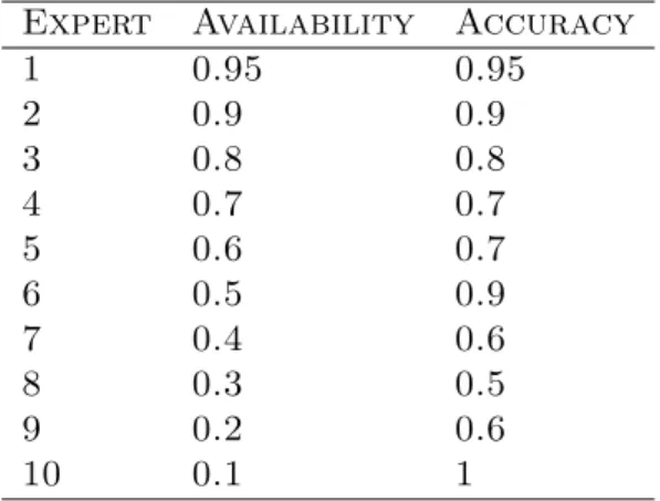
Table 2.1: Availability and accuracy of experts. Expert Availability Accuracy

1 0.95 0.95 2 0.9 0.9 3 0.8 0.8 4 0.7 0.7 5 0.6 0.7 6 0.5 0.9 7 0.4 0.6 8 0.3 0.5 9 0.2 0.6 10 0.1 1

2.4

Experimental Results

In this experiment, we compare the performance of our proposed algorithms to other algo-rithms in this sleeping expert setting. We run algoalgo-rithms on both synthetic dataset and real dataset (Netflix) to prove that our algorithms not only works in the stochastic setting but also in a more general case without any stochastic assumption. First, we consider a synthetic data set consisting of recommendations for objects from 10 experts in 1000 rounds, during which some experts could abstain from voting. The predictions of experts take values in [0,1], while the outcomes (objects) are binary {0,1} generated from a Bernoulli distribu-tion with parameter 0.5. Each expert votes only when he is present, frequency of which depends on his availability. The prediction of an available expert depends on his accuracy. We simulate over the set of availability and accuracy given in table 2.1.

To define the accuracy of an expert, we define a tolerance ρ as follows. Expert i is considered to have a correct prediction if his prediction lies within a distance ρ from the outcome, i.e., |xi_t−yt| ≤ ρ. The accuracy of expert i is then defined by the percentage of time that his recommendations are correct, and is denoted by µi. For example, if an expert

i votes in a system with ρ = 0.3 for 100 rounds and his accuracy µi = 80%, it implies that 80 of his reccommendations satisfy |xi

t−yt| ≤ 0.3. The value of ρ was chosen to be 0.3 in this simulation.

Let A1 and A2 represent our proposed Algorithm 1 and Algorithm 2, respectively, with decreasing step size, ₁₊1_t. We also investigated performance of Algorithm 1 for a fixed step size. Specifically, A1 001 and A1 05 are two other versions of Algorithm 1 when the step size is set equal to 0.01 and 0.5, respectively.

(31)

Dsybil [26] and SBayes [19].

InDsybil, there are two classes of objects: overwhelming and non-overwhelming. An object is identified as overwhelming if sum of the weights of experts voting for it exceeds a threshold

th, otherwise, the object is non-overwhelming. Experts only vote for an object if they believe it is good. If expert i’s prediction for a non-overwhelming object is correct, his weight is increased by wi

t = wit−1α, where α > 1. Correct votes for an overwhelming object do not result in weight change since the votes are not important. Whenever an expert i votes for a bad object, his weight is decreased by wi_t = w_ti₋₁β, where β < 1. In this simulation, we choseα = 5, β = 0.1, th= 11 to optimize Dsybil0s performance.

SBayes[19] is the weight update rule which keeps the weights of sleeping experts unchanged. One difficulty in comparing these algorithms is that the loss definition of each algorithm differs from the others. Therefore, we use a unified common definition of loss which is defined as the total number of mistakes the algorithm makes. In other words, the prediction of the algorithm is quantized to a binary value and is compared with the outcome.

Since SBayes uses the logarithmic loss function, for a more fair comparison, we also add another algorithm, SBayes abs which is an adaptation of SBayes when the loss is an absolute function.

Figure 2.1 depicts losses incurred by the above algorithms when the constant c of A2 is chosen as 0.2. It is shown that A1 and A1 001 suffers the least loss while Dsybil incurs the most loss and SBayes, SBayes abs are in between. In our simulations, we assumed that a given object to be rated is equally likely to be good or bad, i.e., outcomes 0 and 1 are equiprobable. Since inDsybil, good experts only vote for good objects, this algorithm must rely on experts that have not performed well when a bad object is considered. Consequently, it might suffer much loss due to these non-performing experts’ predictions. This is an inherent flaw of the algorithm Dsybil.

Compared to SBayes and SBayes abs, A1 converges slower to the best expert since it uses a decreasing step size in the update rule. This slowness in convergence is deliberate. In SBayes and SBayes abs, the quick convergence to the best expert means that weights of other experts are decreased quickly. Therefore, when the best expert is not available to vote (is sleeping), the algorithm has to choose among experts that all have small weights. The same is not true for A1. When the best expert goes to sleep alternative “nearly best experts”, which have higher weights than the corresponding SBayes0 experts, are available to vote and help the performance of the algorithm.

The fixed step size versions of Algorithm 1 act differently depending on the value of step size. As expected, these algorithms converge faster than A1 which uses a decreasing step size. In fact, for the experimental setup of table 2.1,A1 001 behaves approximately the same

(32)

Figure 2.1: Comparison of loss ofDsybil, SBayes,SBayes abs,A1,A2, A1 001, and

A1 05 when c= 0.2.

asA1 when the constant step size is set small ,0.01, whileA1 05 behaves approximately the same asSBayes absand SBayeswhen the step size is increased to 0.5. The performance of

A2 varies with the choice of valuec. In particular, whencis chosen to be 0.2, its performance is not comparable toA1, as showed in Figure 2.1. We change the constantcto find the value at which A2 can improve its performance. Figure 2.2 illustrates such a case when c= 0.5, in which A2 outperforms all other algorithms.

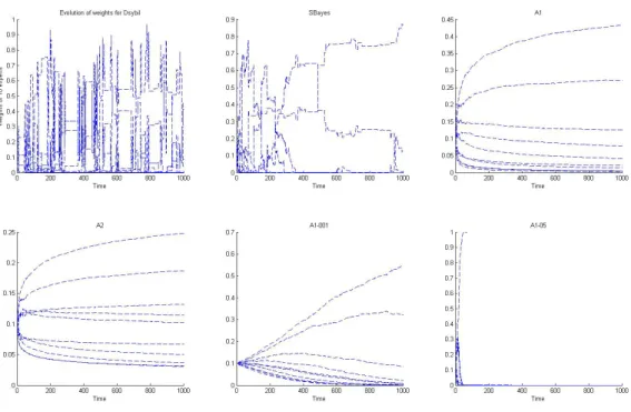
Also in this setting, the weights evolutions of algorithms are investigated. Figure 2.3 shows the weights evolutions of all experts. SinceDsybil use multiplier α= 5 and threshold

th = 11, an expert’s weight of this algorithm could go up to 55 if that expert has been rewarded from the weight roughly the threshold. Therefore, we normalize weights ofDsybil

to obtain the fair comparison with other algorithms. It can be observed that while weights of

Dsybilstill fluctuate after long time, weights ofSBayesconverge much faster. As mentioned above,A1 converges more slowly than SBayes. However, the fixed step size algorithms can increase the convergence rate. Specifically,A 05 converges faster thanA1 001 which is faster

(33)

A1 05 when c= 0.5.

than A1.

In the second part of the simulation, we compare the performance of algorithms on the Netflix dataset. For the purpose of comparing the algorithms’ performance and reduce the running time, we only use a subset of this dataset, including 3153 experts, 14 movies and the voting period is within 2180 days. The predictions of experts are given in the normalized five-star scale {0.2,0.4,0.6,0.8,1}. The outcomes are obtained from feedback of an experienced movie consumer. Figure 2.4 shows the loss comparisons when the constant c of A2 is set equal to 0.2. In this figure, Dsybil again gets the poor performance while A1 and A1 001 still outperform the rest (A1 is slightly better than A1 001). In the experiment with this dataset, SBayes and SBayes abs algorithms perform slightly worse than A1 and A1 001 but still better than A1 05. Note that the number of movies noticeably increases in the time period 1100 to 1500. Therefore, it is more likely that the best expert misses on voting for some of the movies during this time. Algorithms do not solely rely on the best expert in that case such that our algorithms do more favorably in this scenario due to the higher weights

(34)

Figure 2.3: Experts’ weights evolution of algorithms whenc= 0.5.

for other good experts. Since for this dataset, there is no obvious way (at least after some runs with different values ofc) to choose cthe performance of A2 is not good as opposed to its performance on the synthetic data. It is slightly better than Dsybil, but not better than

A1 05 even whencis changed to a better chosen value, e.g., 0.8, as illustrated in Figure 2.5. It has been observed that whileA2 achieves superior performance in stochastic settings with an appropriate choice of constant c, it does not practically seem to guarantee such a good performance in an adversarial setting, e.g., in Netflix dataset. In two cases, A1 and A1 001 always outperform others.

(35)

(36)

(37)

CHAPTER 3

ADVERSARIAL ATTACKING STRATEGIES

In this chapter, we analyze optimal adversarial strategies against the weighted average pre-diction algorithm in the learning with expert advice framework. All but one expert are honest and the malicious expert’s goal is to sabotage the performance of the algorithm by strategi-cally providing dishonest recommendations. We formulate the problem as a Markov decision process (MDP) and analyze it under various settings with two kinds of losses: logarithmic loss and absolute loss.

3.1

Notations and Problem Formulation

Let E = {1,2, ..., N} be the set of experts. At round k, each expert i has a weight pi k−1 ∈ [0,1]. The prediction of expert i is denoted by xi_k ∈ {0,1}. Upon receiving the expert predictions, the algorithm calculates a weighted average prediction, ˆyk. After the prediction is made, the outcome, denoted by yk, is revealed. We assume the outcome is in {0,1}. After the outcome is revealed, the algorithm incurs a loss l(ˆyk, yk) and experti incurs a loss

l(xi

k, yk). The algorithm updates the weights of experts based on the losses they incurred using a multiplicative update rule. The learning process is summarized by Algorithm 3.

In this paper, we only focus on two kinds of losses: • Logarithmic Loss:

l(yk,yˆk) :=−I{yk = 1}ln(ˆyk)−I{yk = 0}ln(1−yˆk). • Absolute Loss: l(yk,yˆk) =|yk−yˆk|.

Note that we can rewrite the logarithmic loss asl(yk,yˆk) =−ln(1−|yk−yˆk|),that will be con-venient for later use. In this case, to avoid the loss function going to infinity, we slightly mod-ify the binary predictions to{,1−}, whereis a small number. We let~pk = (p1k, p2k, ..., pNk) be the state orweight vector of all experts at round k, and ~p˜k = (˜p1k, . . . ,p˜Nk) be the

(38)

corre-Algorithm 3 The weighted average learning algorithm Initialize: pi

0 = 1 for i = 1,2,...,N. for each round k = 1,2, ...do

Nature chooses an outcome. Prediction:

Each expert i predicts xi_k∈ {0,1}. Algorithm predicts ˆyk, ˆ yk = P i∈Ep i k−1xik P i∈Epik−1 . (3.1)

Nature reveals the outcome yk∈ {0,1}. Update:

Each expert’s weight is updated as:

pi_k =pi_k₋₁e−l(xik,yk)_. _(3.2)

end for

sponding normalized weight vector where ˜ pi_k = p i k P i∈Ep i k , i= 1,2, . . . , N (3.3)

is the normalized weight of expert i. Note that we always have P

i∈Ep˜ i

k= 1,∀k.

Throughout this paper, we assume that expert i (i6= 1) makes a correct prediction, i.e., one that agrees with the outcome, with probability µi (the accuracy of experti). That is,

xi_k=

(

yk w.p µi, 1−yk w.p 1−µi.

(3.4) Without loss of generality assume that the malicious expert is expert 1 and recall that all the other experts are honest. We assume expert 1 knows the prediction distribution of each expert i (this can be learned empirically from the history of predictions, for example). Furthermore, at round k, expert 1 knows the true outcome yk and the whole history of predictions up to round k−1. Thus, at round k, the information set given to expert 1 is {yk, y`, xi`, ~p˜`, ` = 1, ..., k −1, i ∈ E}. Based on this information set, this expert selects an action (prediction)x1_k ∈ {T, L}, standing for “truth” or “lie”, whereT :=yk, andL:= 1−yk. After the predictions of all the experts (honest and malicious) are revealed, their weights will be updated according to (3.2). The malicious expert’s program is cast as an MDP1, in

1_{Here, the malicious expert’s action at time}_k_is_x1

k which incurs the lossl(ˆyk, yk), and change the state

~

pk= (p1k, p

2

k, ..., p N

k ) to the next state~pk+1= (p1k+1, p 2

k+1, ..., p

N k+1).

(39)

which, he aims to maximize the expected accumulated loss of the algorithm over the horizon K, i.e., max x1 1,...,x1K K X k=1 Ex2 k,...,xNk(l(ˆyk, yk)), (3.5)

where the expectation is taken over the randomization ofx2

k, ..., xNk, i.e., predictions of honest experts.

Algorithm 4 summarizes the adversary’s optimal policy for the problem defined by (3.5). In Algorithm 4 Adversary’s optimal strategy (DP)

Initialize: VK(.) = cK(.) = 0

for each step k=K−1 downto 1 do Find the optimal action,

u∗_k(yk, ~pk−1) = arg max x1 k c_x1 k(yk, ~pk−1)+EV ∗ k+1(yk+1, φx1 k(~pk−1)) ,

and the corresponding value function,

V_k∗(yk, ~pk−1) = max x1 k c_x1 k(yk, ~pk−1)+EV ∗ k+1(yk+1, φx1 k(~pk−1)) . (3.6) end for Output: sequence u∗_K₋₁(.), V_K∗₋₁(.), ..., u∗₁(.), V₁∗(.). this algorithm, c_x1

k(yk, ~pk−1) denotes the current cost that the adversary can impose on the

system by taking action x1_k and is defined as the expected loss of the algorithm at round k

with respect to actions of the honest experts:

c_x1

k(yk,