Agglomeration effects on labour demand

(1)

No. 28/2006

Agglomeration effects on labour demand

Uwe Blien, Kai Kirchhof, Oliver Ludewig

(2)

Agglomeration effects on labour demand

Uwe Blien, Kai Kirchhof, Oliver Ludewig (IAB)

Auch mit seiner neuen Reihe „IAB-Discussion Paper“ will das Forschungsinstitut der Bundesagentur für Arbeit den Dialog mit der externen Wissenschaft intensivieren. Durch die rasche Verbreitung von Forschungsergebnissen über das Internet soll noch vor Drucklegung Kritik angeregt und Qualität

gesichert werden.

Also with its new series "IAB Discussion Paper" the research institute of the German Federal Employment Agency wants to intensify dialogue with external science. By the rapid spreading of research results via Internet still before printing criticism shall be stimulated and quality shall

(3)

Contents

1 Introduction... 5

2 Background ... 6

3 The Empirical Model... 9

3.1Models for static labour demand ... 9

3.2Models for dynamic labour demand ...11

4 The Data ...12

5 Results...17

6 Conclusion...22

Table 1: Summary statistic of the data set...14

Table 2: Characterization of regions...16

Table 3: Static labour demand, first step: fixed effects – all establishments ...17

Table 4: Static labour demand, second step: analysis fixed effects – all establishments ....18

Table 5: A parsimonious dynamic model (one-step results)...20

(4)

Abstract

How do agglomeration effects influence the demand for labour? To answer this question, approaches on labour demand are linked with an analysis of the classic “urbanization effect”. We use models for static and for dynamic labour demand to find out, whether agglomerations develop faster or slower than other regions. Estimations of the static model show the influ-ence of different degrees of regional concentration at the employment level. The model of dynamic labour demand is used to estimate the effect of different regional types on the growth rate of labour demand.

The empirical results (received with the linked employer-employee data-base of the IAB) on long-run or static labour demand indicate substantial agglomeration effects, since c. p. employment is higher in densely popu-lated areas. In the dynamic model, however, labour demand in core cities grows slower than the average. This is not a contradiction. Labour de-mand is especially high in large cities, but the other areas are slowly re-ducing the gap.

JEL-Classification: J23, R23, R11

The authors thank L. Bellmann, L. Dirnfeldner, A. Furtado, A. Pahnke, H. Sanner, J. Südekum and K. Wolf for very valuable advice. Participants of the 2006 Con-gresses of the European Association of Labour Economists, the European Re-gional Science Association and the German Statistics Association are thanked for valuable hints to an earlier version of this paper. Any responsibility for the analy-sis and the presentation remains with the authors.

(5)

1 Introduction

Empirical and theoretical analyses on labour demand are often carried out without any specific reference to the regional dimension of the labour market. This dimension is, however, of considerable importance, as can be seen from a new debate about the effects of regional concentration on employment. The debate was started by seminal papers in the Journal of Political Economy by Glaeser et al. (1992) and Henderson et al. (1995). There is a new and expanding literature about different kinds of agglom-eration (urbanization/ localization) effects on economic activity which de-rives novel results from ideas dating back even to Marshall. This literature includes contributions from the New Economic Geography (Krugman 1991) and from other theoretical and empirical work.

In this paper we intend a fusion of standard approaches on labour demand with the literature on agglomeration effects. This fusion has its advan-tages: In the literature on agglomeration effects it is normally not possible to control for the exact nature of the externality that gives rise to agglom-eration effects. Here, a detailed analysis of labour demand could give new insights.

On the other hand a labour demand function might be not completely specified if the regional context of a firm is not included. For example, the effects of technological change might be completely different depending on whether the firm operates in a favourable environment or whether it is rather isolated. The diffusion of technological improvements and its effects on employment need to be studied with respect to the regional context. Therefore, this paper uses an integrated approach: A labour demand func-tion is estimated which is extended to take the regional context into ac-count. The data requirements of this approach are rather vast, since data on three levels have to be put together: data on employees, on estab-lishments and on regions. The models used have to take care of the multi-level problem which must be solved to understand the relation between individual organizations and their contexts. Since in this study workers are nested within establishments and establishments within regions, it is neces-sary to observe effects due to the clustering of observations and due to the interaction of levels.

(6)

For the analyses we use the linked employer-employee database of the IAB (called LIAB, see Alda, Bender, Gartner 2005). This includes the IAB Establishment Panel with currently about 16,000 establishments in each of the yearly waves. The IAB Establishment Panel is based on personal inter-views with leading representatives of establishments in the years 1993– 2003. The questionnaire was designed to make available a comprehensive set of information for analyses of the labour market. The sample is repre-sentative for Germany. The panel is linked with data of the employment statistics which includes information about all workers covered by social security. Information about regions is also included in the database. These variables indicate the degree of concentration of economic activity.

2 Background

Currently a debate is going on about the effects of different kinds of ex-ternalities on the regional development of productivity and employment. What economic structure supports employment growth at the local level? Glaeser et al. (1992) argue that a diversified economic structure is advan-tageous, whereas the study of Henderson et al. (1995) finds that own in-dustry specialisation is the major engine of employment growth.

In this paper we are interested in answers to a related, but not identical, question. We intend to study the effects of the size of the respective ag-glomeration, i.e. we look at the classical “urbanization effect”. Due to the typology of Krugman (1991) this is the effect associated with the sheer size of the local agglomeration, without any regard to its specialisation or diversity. In the approaches of New Economic Geography the size of a lo-cal economy is associated with an externality, since the concentration of production generates a concentration of consumers and the latter is fa-vourable for the concentration of production. Therefore, a cumulative cau-sation process gives rise to a centre/periphery structure.

The assumptions of the New Economic Geography are restrictive. Many industries produce for the world market and the local agglomeration of consumers is not very important. Apart from this there are “deglomera-tion” – e.g. congestion – effects working in the opposite direction. In densely populated areas the overcrowding of places has unfavourable con-sequences. Increasing prices of housing, traffic problems, competition of firms for qualified labour etc. increase the cost of production. Therefore, it

(7)

is an empirical question whether agglomerations develop faster or slower than the rural country. Empirical studies undertaken by Möller, Tassi-nopoulos (2000) and Suedekum, Blien, Ludsteck (2006) for Germany show that employment in city centres has smaller growth rates than in the rest of the country.

This research is relevant for an assessment of political measures. In re-cent years older concepts of “growth poles” have been revitalised under new headings. Common to all these concepts is the proposition that a suc-cessful development policy should be concentrated on the large cities. This is behind the new emphasis placed on “Metropolitan Regions” in European (and in German) development programmes. It is at least part of the “clus-ter” concept on regional growth, since one of the meanings given to the rather evasive cluster term is “pure agglomeration” (McCann 2005). There has been a change in the direction of regional assistance programmes, since these are now oriented towards the most likely growth engines of the country and not towards fair regional distribution of economic activi-ties. The assumption is that there are secondary effects working in favour of the rural country. These include spillovers from the centres. The Metro-politan Regions are expected to pull the other parts of the country to higher levels of growth. But there is doubt about the effectiveness of all these programmes. How could an agglomeration produce spillovers effec-tive for growth if its own growth rate is smaller than the one of the rest of the country?

In many empirical tests agglomeration effects are measured using a pure cross-section approach, as long-run employment growth rates are re-gressed on control variables that reflect the regional industry composition in some base year.1_{It is thus assumed that a historical pattern from 10–} 30 years ago affects employment growth, but no real test is provided about the relevant time structure. To be able to do such test, one needs data of local industries for many consecutive years in order to make full use of the three dimensions of the panel (location, industry, time period). An additional advantage of panel techniques is the possibility to controlfor

1

Both Glaeser et al. (1992) and Henderson et al. (1995) are cross-sections, as well as

the influential study on France by Combes (2000). Among this literature is also the paper by Blien and Suedekum (2005) on Germany (1993–2001).

(8)

time-invariant fixed effects that cannot be easily disentangled from the impact of the local economic structure in a cross-section analysis. This lit-erature normally uses aggregated data on individual workers. Many con-trolling variables measured at the level of establishments that are re-quired to estimate a standard labour demand function are ignored.

We are interested in filling this gap. Our model of labour demand follows the classic work of Hamermesh (1986, 1993) and Nickell (1986). A pro-duction function with capital and labour as the two input factors and the common properties is assumed. A firm trying to minimize costs for a given output will set the optimal level of capital and labour so that the marginal productivity of each factor equals its price. Taking the ratio of these first order conditions one obtains that the marginal rate of technical substitu-tion equals the factor-price ratio in the optimum. This result can now be used together with the output constraint to derive the demand functions for capital and labour.

A simple case for specifying a labour demand function for an empirical model is to use a linear homogeneous production function of the following kind:

(

)

ρ ρ ρ _α α 1 ]1 [ L K A Y = + − . (1)

There Y is the output of a specific firm, L is labour and K is capital. 1 > α > 0, 1 ≥ ρ ≥ -∞ and A is a technology parameter. Minimizing costs subject to a given Output yields the labour demand equation (Hamermesh 1986): Y w A L α ρ −ρ − − − = 1 1 1 1 1 . (2)

Taking logarithms results in a first approach to the linear function of the empirical model: ρ σ σ α − = − + − = 1 1 : with ln ln ln ' lnL w Y A (3)

This is a very simple function, which could be easily estimated. A problem is that the assumptions about the production process might not be exactly met. For example, the production function might not exactly show con-stant returns to scale. Therefore, it is advisable to use an estimation strat-egy which is robust against violations of the basic assumptions. At any rate it is necessary to extend the estimated function with respect to

(9)

re-gional characteristics and other controlling variables. Agglomeration ef-fects could be thought to be working through the parameter A. Depending on regional characteristics labour demand might be higher or lower than the average.

3 The Empirical Model

In our empirical work two different versions of the labour demand function are applied. One is the static version giving the demand in the long run. The other one is the dynamic function which includes lags of the endoge-nous variable. One basic difference between the two specifications is that within static models parameters are estimated that concern the change in labour demand due to the long-run effects of external changes, whereas the dynamic model shows the growth of labour demand. Appropriately adapted static models show agglomeration effects with respect to the level of labour demand, whereas from the dynamic model the response in terms of the growth rate can be obtained.

In many cases it is regarded as unavoidable to estimate dynamic models because normally there is inertia in the development of labour demand. Then, a correctly specified model would include the lagged endogenous variable. In this case the standard fixed effects estimator could not be used, because it gives biased and inconsistent results (Baltagi 2001). In-stead a GMM-estimator has to be applied (Arellano, Bond 1991).

3.1 Models for static labour demand

All these models have to be adapted for the question at hand. In the case of the static function the fixed-effects estimator, commonly used to con-trol for unobserved heterogeneity, allows identifying differences across establishments, which might be caused by regional variables. Hence, we apply a two-step procedure to identify the effects of regional agglomera-tions on the labour demand of establishments. In the first step we use the panel structure of the data to extract the establishment fixed effect from a usual static labour demand function. We do so using the common within estimator. This is the first step equation:

ln

ln ln

lnLit =β0 +βw wit +βY Yit +βX Xit +γt +εit +νi (4)

Here i is the index for the establishment and t the index of time. X is a vector of time-varying variables which are added to equation (3) as

(10)

addi-tional controls. εi,t is the usual error term.γt is a vector of time dummies for the influence of the business cycle and νi is the establishment fixed ef-fect which reflects all time-invariant efef-fects specific to the establishments. This includes things like a favourable location, an especially talented owner and market position within the industry as well as the influence of the regional conditions as summarized in agglomeration or suburbaniza-tion effects. Therefore the effect of the variable A in equasuburbaniza-tion (3) is in-cluded in the fixed effect νi. Since most establishments do not change their respective region a second step is required to identify agglomeration effects. The fixed effects are regressed to type of regions, some spell indi-cators and other firm-specific and time-constant variables Z:

ln ' _i 0 i β βrDr βZ Z βSSt ηi ν = − + + + (5)

The Ds are dummies which represent the type of the respective region. Formally, they partly replace the parameter A of the theoretical model, which could have positive or negative effects on employment. The Ds should represent the information about the degree of agglomeration which is characteristic for the region.

Using unbalanced panel data we have to add a further set of special con-trols. Due to the unbalanced time structure the different νi are determined on the basis of different observation spells. Some establishments are ob-served from 1995 to 2001, others from 1996 to 1999 and so on. Thus dif-ferent conditions at certain points of time and difdif-ferent observations spells might influence the value of νi for each firm. We control for this by defin-ing a dummy variable for each spell length and an interactdefin-ing term with the diverse wave dummies yielding 21 spell indicators (S). These are added to the regression function of the second step.

Besides these spell dummies and our main explanatory variable, the re-gional type in which an establishment is located, we add a set of control variables Z which are fixed over time or quasi-fixed. Quasi-fixed variables are those which only change for very few establishments at a point of time or very seldom or by very small amounts, like the existence or not-existence of a works council, or the industry or fraction of certain em-ployee groups. Whether a variable is quasi-fixed or free over time is a matter of degree.

(11)

One final remark on this procedure: In the first step the coefficient βY is expected to be close to one. This might be not the case if the variable Y does not vary much in time. In this case part of its effect is included in the fixed effect.

3.2 Models for dynamic labour demand

If there is considerable inertia in the adaptation process a dynamic model might be appropriate for labour demand. In this case the lagged endoge-nous variable is included:

ln ln ln ln lnL_it =

β

₀ +

β

_L L_i₍_t₋₁₎ −

β

_w w_it +

β

_Y Y_it +

β

_X X_it +

γ

_t +

ε

_it +

ν

_i (6)

In principle the same two-step procedure could be used as in the static model. But we change the procedure to obtain information not only about agglomeration effects on the level of labour demand but also on its growth. This could be done in the following way. With GMM the above equation is differenced to eliminate the fixed effects. In this case the equation is formulated in differences of logs, i.e. in approximations of growth rates. It would be informative to have the effect of agglomerations on the growth rate of labour demand. This could be done by including a specific trick introduced by Nickell et al. (1992). To avoid the elimination of the time-invariant variables, they included interactions of time-constant variables with a time index t. We do the same:

ln ln ln ln lnL_it =

β

₀ +

β

_L L_i₍_t₋₁₎ −

β

_w w_it +

β

_Y Y_it +

β

_X X_it +t

β

_rD_r +

γ

_t +

ε

_it +

ν

_i (7)

Now we gain the effect of a time-constant dummy variable representing the type of the respective region (in which the establishment i is located) on the growth rate of labour demand. No second step is required. Since equation (7) is estimated by taking differences, the effect of a special de-gree of agglomeration on the growth rate of labour demand is estimated. This is more closely related to the current literature on agglomeration ef-fects than the estimates obtained with the static model.

In a last remark we address the multilevel structure of the problem. Moul-ton (1990) is famous for showing that the inclusion of variables related to different levels of observation, here regions and establishments, could re-sult in inefficient estimates of the coefficients and in biased estimates of the standard errors especially of the variables measured at the higher level. He recommends the inclusion of fixed effects for the higher-level

(12)

units. This is redundant in our case since we include fixed effects for es-tablishments. If there were no relocation of establishments, regional fixed effects would be perfectly multicollinear with establishment fixed effects. In our case with rare movement of establishments they are highly multi-collinear.

4 The Data

We use the so called IAB Establishment Panel (IAB-Betriebspanel, see Bellmann 1997 and Kölling 2000) as one basic data source. It is extended to a employer-employee linked panel by linking it with the employment statistics of Germany. The IAB Establishment Panel is a general purpose survey based on a random sample giving longitudinal information in yearly waves for the time since 1993 in West Germany and since 1996 for East Germany. It contains a broad range of variables regarded as important in economic theory. It includes establishments of all sizes, and is not re-stricted to manufacturing. These basic structural elements correspond to some of the principles of an ideal set of establishment data suggested by Hamermesh (1993). An establishment as it is counted in the panel is the local plant of a firm. It might be identical with the entire firm or it might be a part of it.

Starting with 4,300 establishments, the sample size of the survey was ex-tended in several steps. Currently, it covers about 16,000 establishments in its yearly waves. Most of the information is collected by trained inter-viewers. Only in some regions the sample size is extended by data collec-tion through mailed quescollec-tionnaires. The base populacollec-tion consists of all es-tablishments with at least one employee covered to the compulsory social security system. Over 80% of the German establishments fulfil this condi-tion. Since the survey is supported by the German employers’ association and Federal Labour Agency (Bundesagentur für Arbeit), there is a rather high response rate of around 70% for initial contacts and about 80% for the annually repeated contacts. The establishment panel provides general information on the establishments, such as organizational practices, total sales, employment or the industrial relations within the establishment. The second data set is the so called Employment Statistics (Beschäftigten-Leistungsempfänger-Datei). This is a database generated for administra-tive purposes and therefore especially reliable. Pensions are computed

(13)

from the original data. All employees are included who are covered by the social security system. This database comprises information on gender, wage, age, occupation and qualification of the employees. Thus a rich per-sonalized database is generated.

The IAB Establishment Panel and the Employment Statistics are linked (forming the LIAB) by a unique establishment identification number. Thus it is possible to match the information of all employees covered by the so-cial security system with the establishments of the IAB Establishment Panel. In doing so, we add the averages across an establishment of vari-ables from the employment statistics as new varivari-ables to the establish-ment panel. Variables giving establishestablish-ment characteristics, like total sales or existence of a works council, stem from the establishment data.

The establishment panel starts in 1993. We use data of the Employment Statistics Registry until 2002. Thus our time window is ranging from 1993 to 2002. However, some questions of the survey are backward looking, such as “What were your total sales last year?” Thus we have to transfer some of the information of t+1 to t, generating missings for establish-ments not observed in t+1.

The panel is unbalanced due to panel mortality, missing values on some variables and new entrants to the panel. Therefore it is necessary to con-trol the effects of different observation times and spell lengths. We do so by introducing time dummies in the first step analysis and the spell indica-tors described above in the second step analysis.

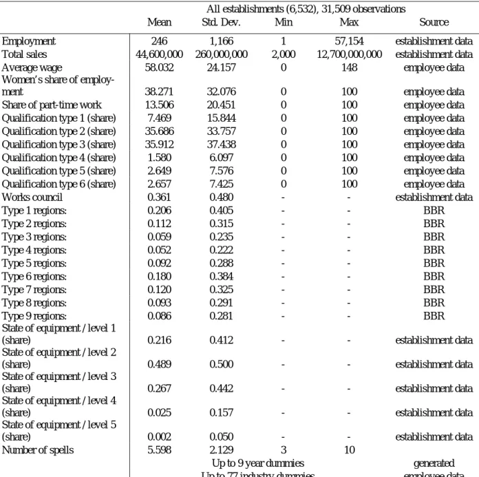
While this data set is rather large and representative for Germany it is not possible to use all observations. We exclude the agricultural and mining sector, non-profit organisations and state agencies as well as observations with missing values on variables used in the estimations. Establishments with only one or two observations are also excluded to get a broader base for the fixed effects estimator. This leaves us with 6,532 establishments observed over an average of 4.8 waves, giving a total of 31,509 observa-tions. The minimum length of a spell is 3 years, the maximum length is 10 years. Table 1 gives the descriptive statistics of the variables used and indicates the source data set.

(14)

Table 1: Summary statistic of the data set

All establishments (6,532), 31,509 observations

Mean Std. Dev. Min Max Source

Employment 246 1,166 1 57,154 establishment data

Total sales 44,600,000 260,000,000 2,000 12,700,000,000 establishment data

Average wage 58.032 24.157 0 148 employee data

Women’s share of

employ-ment 38.271 32.076 0 100 employee data

Share of part-time work 13.506 20.451 0 100 employee data

Qualification type 1 (share) 7.469 15.844 0 100 employee data

Works council 0.361 0.480 - - establishment data

Type 1 regions: 0.206 0.405 - - BBR Type 2 regions: 0.112 0.315 - - BBR Type 3 regions: 0.059 0.235 - - BBR Type 4 regions: 0.052 0.222 - - BBR Type 5 regions: 0.092 0.288 - - BBR Type 6 regions: 0.180 0.384 - - BBR Type 7 regions: 0.120 0.325 - - BBR Type 8 regions: 0.093 0.291 - - BBR Type 9 regions: 0.086 0.281 - - BBR

State of equipment / level 1

(share) 0.216 0.412 - - establishment data

Number of spells 5.598 2.129 3 10

Up to 9 year dummies generated

Up to 77 industry dummies employee data

Let’s take a closer look on the variables. As mentioned above, the wage variable is taken from the registry data and averaged across employees of each establishment. The qualification level of each employee is also pro-vided by the registry data. The qualification levels are increasing from one (low skilled) to 6 (university degree). Employees without information about their qualification are put into the category 7. These are mostly un-skilled persons. We calculated the shares of each qualification level for each establishment. The same procedure was conducted with the women’s share and the share of part time employees.

(15)

We use also the industry classification of the registry data, since it is more detailed than the one of the establishment panel and since the IAB estab-lishment panel is providing one set of industry classification until 1999 and another one from 2000 onwards. The industry classification is used to generate 77 dummies. The share of the service sector establishments, which is about 43% of all observations, is also calculated using the indus-try classification. The share of West German establishments (57% of all observations) is calculated on the basis of the employee data, which pro-vides the regional location of the workplace. The industry structure might be very important with respect to differing patters of product demand and technical progress which influence employment (cf. Blien, Sanner 2006). The establishment panel also provides very important variables. The em-ployment of the establishment is one, also total sales. Another variable reflects an important feature of industrial relations in Germany. This is a dummy indicating the existence of a works council. It is coded 1 (a works council exists) and 0 (no works council). 36% of the observations have a works council. Since this variable is asked biannually, every second year is missing. We circumvent this problem by relying on the substantial inertia of such an institution and fill the missing values in t+1 with values for t. The state of equipment is a categorical variable which reflects the moder-nity of the real capital. It is ranging from one (state of the art) to five (out-dated). We use one as reference category and insert dummies for the four remaining levels into (some of) our empirical specifications.

Spell length indicates the number of observations per establishment. The average based on all observations is 5.6. This is more than the average number of waves calculated above on basis of the number of establish-ments, because establishments with longer spells provide by definition more observations. Depending on the length of the spells and their start-ing point we define up to 21 identifiers of spells with different length and starting years. These spell identifiers enter as dummies into our estima-tion.

In addition to information about individual workers and establishments data on regions are used for the analysis. In fact, this is the most important in-formation for the research question. To analyze the effects of economic concentration, appropriate regional units have to be defined first. If large or heterogeneous regions were used, the effects would be blurred. To avoid

(16)

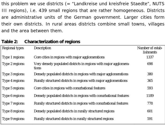
this problem we use districts (= “Landkreise und kreisfreie Staedte”, NUTS III regions), i.e. 439 small regions that are rather homogeneous. Districts are administrative units of the German government. Larger cities form their own districts. In rural areas districts combine small towns, villages and the area between them.

Table 2: Characterization of regions

Regional types Description Number of

estab-lishments Type 1 regions: Core cities in regions with major agglomerations 1337 Type 2 regions: Very densely populated districts in regions with major

agglomera-tions

698 Type 3 regions: Densely populated districts in regions with major agglomerations 380 Type 4 regions: Rurally structured districts in regions with major agglomerations 365 Type 5 regions: Core cities in regions with conurbational features 593 Type 6 regions: Densely populated districts in regions with conurbational features 1189 Type 7 regions: Rurally structured districts in regions with conurbational features 778 Type 8 regions: Densely populated districts in rurally structured regions 601 Type 9 regions: Rurally structured districts in rurally structured regions 591

(Classification following Goermar and Irmen 1991)

To map agglomeration effects a widely used classification of German dis-tricts (Goermar and Irmen 1991) provided by the Federal Office for Build-ing and Regional PlannBuild-ing (BBR) is adopted. As can be seen from Table 2 the classification is based on the density of the population and the central-ity of the location. We define eight dummy variables indicating the types 2 to 9. Thus, we are using the core cities in regions with major agglomera-tions as the reference category. These are cities with at least 300,000 in-habitants.

The use of the typology in table 2 has advantages compared to the direct inclusion of single indicators like population density or population size. These variables often give an erroneous picture of the regional units. The definition of regions does not follow a stringent criterion, but historical idiosyncrasies and administrative purposes applied differently in different part of the country. Population density might vary very much for a core city, since in one case the surrounding country is included in others not.

(17)

5 Results

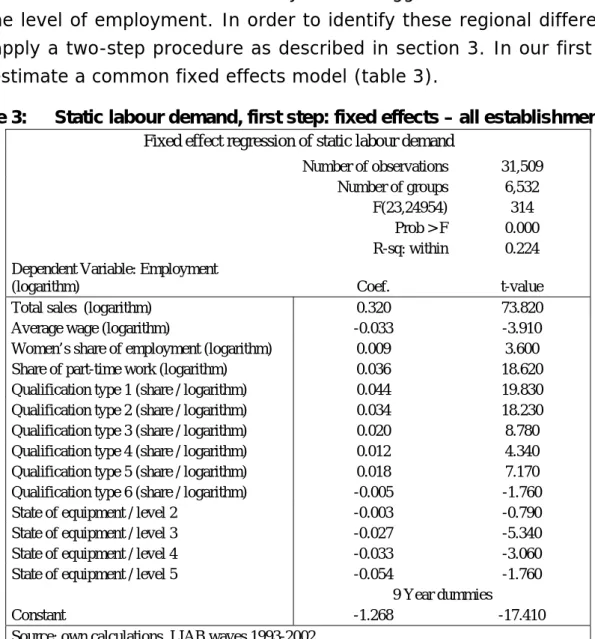
The model for static or long run labour demand gives a first impression of differences between the rural country and the agglomerations with respect to the level of employment. In order to identify these regional differences we apply a two-step procedure as described in section 3. In our first step we estimate a common fixed effects model (table 3).

Table 3: Static labour demand, first step: fixed effects – all establishments

Fixed effect regression of static labour demand

Number of observations 31,509 Number of groups 6,532

F(23,24954) 314

Prob > F 0.000

R-sq: within 0.224

Dependent Variable: Employment

(logarithm) Coef. t-value

Total sales (logarithm) 0.320 73.820

Average wage (logarithm) -0.033 -3.910

Women’s share of employment (logarithm) 0.009 3.600

Share of part-time work (logarithm) 0.036 18.620

Qualification type 1 (share / logarithm) 0.044 19.830

Qualification type 6 (share / logarithm) -0.005 -1.760

State of equipment / level 2 -0.003 -0.790

9 Year dummies

Constant -1.268 -17.410

Source: own calculations, LIAB waves 1993-2002

The coefficients of total sales and wages have the right sign; however, the coefficient of total sales is relatively small. As discussed above this might be due to the fact that the fixed effect is capturing part of this relation-ship. Estimating the same function without fixed effects yield coefficients about 0.8 for total sales, thus, supporting our hypothesis. Since our focus is not the coefficients of the labour demand equation, we include fixed ef-fects to control for unobserved heterogeneity.

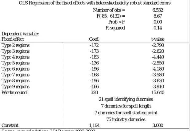
In the second step the fixed effects estimated in the first step are re-gressed on the regional types described above and on some control vari-ables (table 4).

(18)

Table 4: Static labour demand, second step: analysis fixed effects – all establishments

OLS Regression of the fixed effects with heteroskedasticity robust standard errors

Number of obs = 6,532

F( 85, 6132) = 8.67

Prob > F 0.00

R-squared 0.14

Dependent variable:

Fixed effect Coef. t-value

Type 2 regions -172 -2.790 Type 3 regions -173 -2.620 Type 4 regions -183 -4.440 Type 5 regions -136 -2.550 Type 6 regions -196 -4.180 Type 7 regions -168 -3.580 Type 8 regions -196 -3.630 Type 9 regions -166 -3.910 Works council 320 15.640

21 spell identifying dummies 7 dummies for spell length 7 dummies for spell starting point

75 industry dummies

Constant 1,194 3.000

Source: own calculations, LIAB waves 1993-2002

To facilitate interpretation of the results we use a transformed version of the fixed effects. The first-step equation is in logs, therefore we use the exponentiated values of the fixed effects.2_{Additionally to our regional} types we include the works council variable as well as 75 industry dum-mies and 21 spell identifier as time invariant control variables.

All coefficients of the regional dummies are negative and significant. The reference category is core cities in large agglomerations. Thus, ceteris paribus the employment level of establishments located there is on aver-age higher than the level in other regions. This might concern employ-ment in general. Another explanation would be that many firms localize their headquarters, central administrations, central development units in large cities, whereas plants with reduced functions are placed elsewhere. This might be due to the person-to-person contact that is required with units close to the external market. It is also necessary with development units which are appropriately placed in locations with other firms and uni-versities.

2_{The second step with fixed effects which are not transformed gives basically the same}

(19)

Thus, the static analysis of labour demand gives agglomeration effects. Congestion effects seem to be smaller than the advantages of a large city, at least with respect to the employment criterion. On a first glance the agglomeration hypothesis is supported.

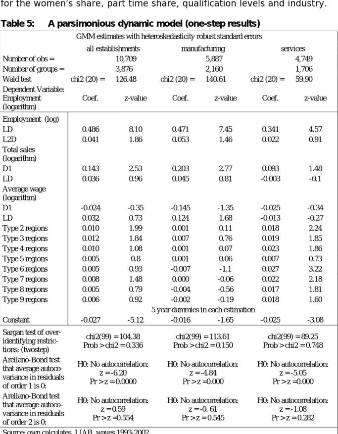
Now we look at the effects of agglomerations on employment growth in a dynamic model, applying the mentioned trick of Nickell et al. (1992). Us-ing the dynamic approach has the additional advantage of takUs-ing care of possible inertia in labour demand of the individual firms. We estimate two versions of the dynamic panel model with the Arellano-Bond estimator. The first is a rather parsimonious model. We only include total sales, wages (both in logs), wave dummies and the regional types in addition to the lagged values of the dependent variable. Total sales and average wages are instrumented by lags of their own levels. Thus we are account-ing for the predetermination of wages and sales.3_{This model specification} is then applied to three different (sub-)samples: all establishments, only manufacturing and only services.

The results (table 5) for the whole sample and for services include coeffi-cients for the region types which are positive indicating that average em-ployment growth is greater for all establishments not located in core cities in regions with major agglomerations. However, for the whole sample only the coefficients on regional type 2 and 3 are (weakly) significant. Thus es-tablishments in areas in the vicinity of large agglomerations are growing especially fast (or are shrinking slower than average).

For the service sector almost all coefficients are significant. Employment in the service sector is developing better in all regional types than in the core cities. This effect is especially strong in densely populated districts in re-gions with conurbational features. These results show suburbanization processes.

The findings with respect to the manufacturing sector are inconclusive. The larger part of the coefficients is positive, but they are all insignificant.

3_{The predetermination assumption of these variables is supported by a substantial}

higher p-value of the Sargan test compared to a model with wages and sales as strictly exogenous variables.

(20)

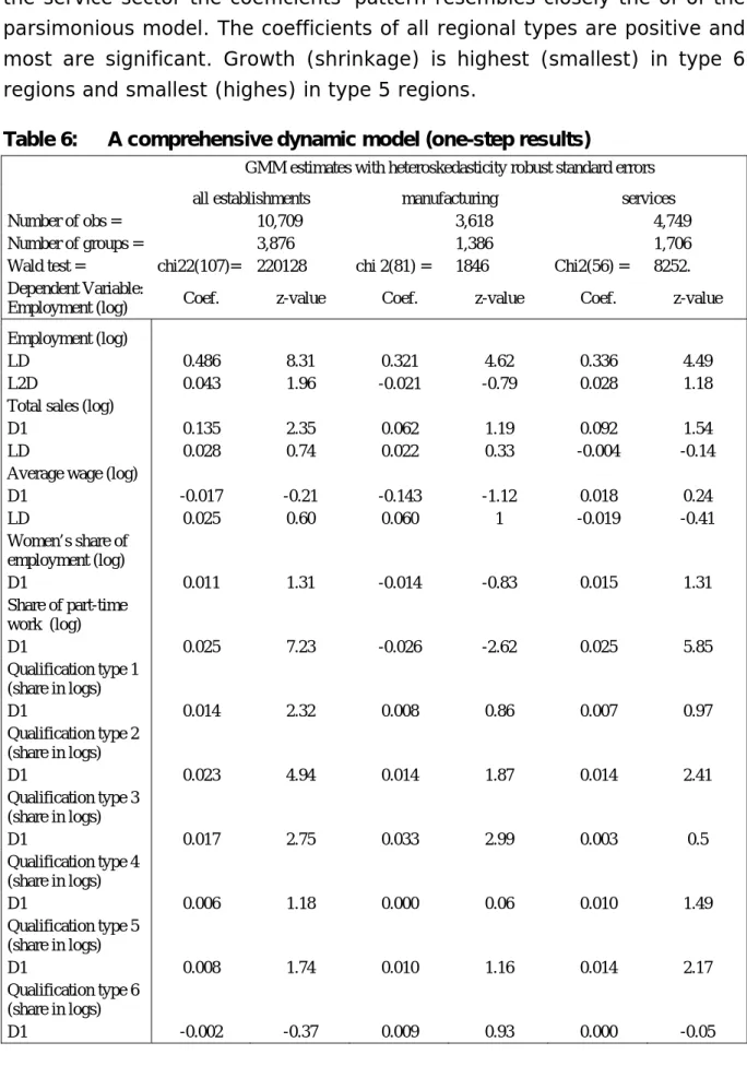
However, these results might be affected by an omitted variable bias. Therefore we estimate a more comprehensive model. We include controls for the women’s share, part time share, qualification levels and industry.

Table 5: A parsimonious dynamic model (one-step results)

GMM estimates with heteroskedasticity robust standard errors

all establishments manufacturing services

Number of obs = 10,709 5,887 4,749

Number of groups = 3,876 2,160 1,706

Wald test chi2 (20) = 126.48 chi2 (20) = 140.61 chi2 (20) = 59.90 Dependent Variable:

Employment (logarithm)

Coef. z-value Coef. z-value Coef. z-value

Employment (log) LD 0.486 8.10 0.471 7.45 0.341 4.57 L2D 0.041 1.86 0.053 1.46 0.022 0.91 Total sales (logarithm) D1 0.143 2.53 0.203 2.77 0.093 1.48 LD 0.036 0.96 0.045 0.81 -0.003 -0.1 Average wage (logarithm) D1 -0.024 -0.35 -0.145 -1.35 -0.025 -0.34 LD 0.032 0.73 0.124 1.68 -0.013 -0.27 Type 2 regions 0.010 1.99 0.001 0.11 0.018 2.24 Type 3 regions 0.012 1.84 0.007 0.76 0.019 1.85 Type 4 regions 0.010 1.08 0.001 0.07 0.023 1.86 Type 5 regions 0.005 0.8 0.001 0.06 0.007 0.73 Type 6 regions 0.005 0.93 -0.007 -1.1 0.027 3.22 Type 7 regions 0.008 1.48 0.000 -0.06 0.022 2.18 Type 8 regions 0.005 0.79 -0.004 -0.56 0.017 1.81 Type 9 regions 0.006 0.92 -0.002 -0.19 0.018 1.60

5 year dummies in each estimation

Constant -0.027 -5.12 -0.016 -1.65 -0.025 -3.08

Sargan test of over-identifying restric-tions: (twostep) chi2(99) = 104.38 Prob > chi2 = 0.336 chi2(99) = 113.61 Prob > chi2 = 0.150 chi2(99) = 89.25 Prob > chi2 = 0.748 Arellano-Bond test

that average autoco-variance in residuals of order 1 is 0: H0: No autocorrelation: z = -6.20 Pr > z = 0.0000 H0: No autocorrelation: z = -4.84 Pr > z =0.000 H0: No autocorrelation: z = -5.05 Pr > z =0.000 Arellano-Bond test

that average autoco-variance in residuals of order 2 is 0: H0: No autocorrelation: z = 0.59 Pr > z =0.554 H0: No autocorrelation: z = -0. 61 Pr > z = 0.545 H0: No autocorrelation: z = -1.08 Pr > z = 0.282 Source: own calculates, LIAB, waves 1993-2002

Despite substantial changes in the model specification, the results are re-markably stable. For the total sample all coefficients of the regional types are positive and those for the type 2 and 3 regions are significant. Thus,

(21)

employment of establishments develops better outside the most populated areas and is strongest in the second and third most aggregated areas. For the service sector the coefficients’ pattern resembles closely the of of the parsimonious model. The coefficients of all regional types are positive and most are significant. Growth (shrinkage) is highest (smallest) in type 6 regions and smallest (highes) in type 5 regions.

Table 6: A comprehensive dynamic model (one-step results)

GMM estimates with heteroskedasticity robust standard errors

all establishments manufacturing services

Number of obs = 10,709 3,618 4,749

Number of groups = 3,876 1,386 1,706

Wald test = chi22(107)= 220128 chi 2(81) = 1846 Chi2(56) = 8252. Dependent Variable:

Employment (log) Coef. z-value Coef. z-value Coef. z-value

Employment (log)

LD 0.486 8.31 0.321 4.62 0.336 4.49

L2D 0.043 1.96 -0.021 -0.79 0.028 1.18

Total sales (log)

D1 0.135 2.35 0.062 1.19 0.092 1.54

LD 0.028 0.74 0.022 0.33 -0.004 -0.14

Average wage (log)

D1 -0.017 -0.21 -0.143 -1.12 0.018 0.24 LD 0.025 0.60 0.060 1 -0.019 -0.41 Women’s share of employment (log) D1 0.011 1.31 -0.014 -0.83 0.015 1.31 Share of part-time work (log) D1 0.025 7.23 -0.026 -2.62 0.025 5.85 Qualification type 1 (share in logs) D1 0.014 2.32 0.008 0.86 0.007 0.97 Qualification type 2 (share in logs) D1 0.023 4.94 0.014 1.87 0.014 2.41 Qualification type 3 (share in logs) D1 0.017 2.75 0.033 2.99 0.003 0.5 Qualification type 4 (share in logs) D1 0.006 1.18 0.000 0.06 0.010 1.49 Qualification type 5 (share in logs) D1 0.008 1.74 0.010 1.16 0.014 2.17 Qualification type 6 (share in logs) D1 -0.002 -0.37 0.009 0.93 0.000 -0.05

(22)

Table 6 continued Type 2 regions 0.009 1.87 0.000 -0.01 0.018 2.41 Type 3 regions 0.014 2.08 0.007 0.74 0.018 1.82 Type 4 regions 0.012 1.26 0.032 2.52 0.020 1.63 Type 5 regions 0.005 0.77 0.004 0.43 0.008 0.81 Type 6 regions 0.005 0.97 0.008 0.94 0.025 3.09 Type 7 regions 0.009 1.52 0.006 0.66 0.019 2 Type 8 regions 0.006 0.89 0.009 0.86 0.019 2.04 Type 9 regions 0.004 0.64 0.013 1.14 0.014 1.32

5 year dummies in each estimation

Industry dummies 68 43 24

constant -0.020 -3.49 -0.030 -2.88 -0.019 -3.03

Sargan test of over-identifying restric-tions: (twostep) chi2(99) = 97.53 Prob > chi2 = 0.523 chi2(99) = 115.07 Prob > chi2 = 0.129 chi2(99) = 82.81 Prob > chi2 = 0.879 Arellano-Bond test

that average autoco-variance in residuals of order 1 is 0: H0: no autocorrelation: z = -6.25 Pr > z = 0.000 H0: no autocorrelation: z = ---2,84 Pr > z = 0.005 H0: no autocorrelation z = -5.16 Pr > z = 0.000 Arellano-Bond test

that average autoco-variance in residuals of order 2 is 0: H0: no autocorrelation z = 0.60 Pr > z = 0.547 H0: no autocorrelation: z = -0.44 Pr > z = 0.660 H0: no autocorrelation z = 1.25 Pr > z = 0.211 Source: own calculates, LIAB, waves 1993-2002

Evaluating the test statistics our specifications are mainly supported. The Sargan test of over identification (calculated by a two-step estimation) does not reject the assumption of the exogeneity of the instruments. The Arellano-Bond tests of autocorrelation indicate that in all cases there is as assumed autocorrelation of the first but not of the second order.

6 Conclusion

In this paper we do research on the open question about regional agglom-eration effects on labour demand at the establishment level. For this pur-pose we use the LIAB, a German linked employer-employee database of the Institute for Employment Research (IAB). Applying two different em-pirical approaches we find that establishments within agglomerated re-gions c.p. have a higher employment level. Thus the Krugman hypothesis of agglomeration effects and local demand is confirmed to some extent. This is underlined by the fact that the effect is primarily driven by ser-vices, which are related to local and regional needs – at least to some de-gree. The inconclusive evidence for the manufacturing sector might be ex-plained by the global nature of the demand for most of the goods.

(23)

However, these findings reflect the state of the observation period which is the result of past developments. To gain answers about current devel-opments we estimate a dynamic model. In this context, employment growth rates are smallest for establishments within large agglomerations. Establishments in less populated areas grow faster (or shrink slower). Thus, in accordance with other studies about the German labour market, we observe deglomeration and suburbanization processes. This is driven by the service sector, which is plausible because service sector establish-ments are easier to relocate than manufacturing plants. Due to the gen-eral growth of services there are more opportunities to start new enter-prises for which new locational decisions are required.

There is no conflict between the findings obtained with the static and with the dynamic model. Assuming that the level of employment reflects past decisions, the agglomeration effects of our first empirical approach are results of location decisions made a long time ago, when transportion and communication costs were much higher than today. But due to path de-pendence these former decisions still form the economic structure of to-day.

However, current developments are more strongly influenced by the cur-rent environment. Thus, due to low transportion and communication costs the congestion effects of agglomerations outweigh their advantages. Em-ployment is primarily growing in establishments in less crowded areas. This implies that policy measures focusing on metropolitan areas might not follow the most promising approach.

References

Alda, Holger; Bender, Stefan; Gartner, Hermann (2005): The linked em-ployer-employee dataset created from the IAB establishment panel and the process-produced data of the IAB (LIAB). In: Schmollers Jahrbuch. Zeitschrift für Wirtschafts- und Sozialwissenschaften, Jg. 125, H. 2. pp. 327-336.

Arellano, Manuel; Bond, Stephen (1991): Some Tests of Specification for Panel Data: Monte Carlo Evidence and an Application to Employment Equations. Review of Economic Studies, v. 58, iss. 2, pp. 277-297. Baltagi, Badi H. (2001): Econometric Analysis of Panel Data (Second

(24)

Bellmann, Lutz (1997): The IAB establishment panel with an exemplary analysis of employment expectations. IAB Labour Market Research Topics, No. 20, pp. 1-14.

Blien, Uwe; Sanner, Helge (2006): Structural Change and Regional Unemployment, IAB-Discussionpaper.

Blien, Uwe; Suedekum, Jens (2005): Local economic structure and indus-try development in Germany, 1993-2001. IAB-Discussionpaper.

Blien, Uwe; Suedekum, Jens; Wolf, Katja (2005): Local Employment Growth in West Germany: A Dynamic Approach. Paper presented at the EALE/ SOLE Conference 2005 in San Francisco, forthcoming in: Labour Economics.

Combes, Pierre-Philippe; Magnac, Thierry; Robin, Jean-Marc (2004): The Dynamics of Local Employment in France. Journal of Urban Economics 56, pp. 217-243. reprinted: Discussions Paper Series of Centre for Eco-nomic Policy Research No. 3912 (2004).

Glaeser, Edward L. (1992): Growth in Cities. Journal of Politcal Economy, v. 100, iss. 6, pp. 1126-1152.

Görmar, Wilfried; Irmen, Eleonore (1991): Nichtadministrative Gebiets-gliederungen und -kategorien für die Regionalstatistik. Die siedlungs-strukturelle Gebietstypisierung der BfLR, In: Raumforschung und Raum-ordnung, 49/6, pp. 387-394.

Hamermesh, Daniel S. (1986): The Demand for Labor in the Long Run. In: O. Ashenfelter and R. Layard, eds., Handbook of Labor Economics, North-Holland Press, pp. 429-471.

Hamermesh, Daniel S. (1993): Labor Demand. Princeton and Chichester, U.K.: Princeton University Press.

Henderson, Vernon; Kuncoro, Ari; Turner, Matt (1995): Industrial Devel-opment in Cities. Journal of Political Economy, v. 103, iss. 5, pp. 1067-1090.

Kölling, Arnd (2000): The IAB-Establishment Panel. Schmollers Jahrbuch. Zeitschrift für Wirtschafts- und Sozialwissenschaften, Jg. 120, H. 2,. pp. 291-300.

Krugman, Paul (1991): Geography and Trade, Cambridge (Mass.) etc.: MIT Press.

McCann (2005): Industrial Clusters. Paper presented at the Conference on Regional Development, University of Barcelona.

Möller, Joachim; Tassinopoulos, Alexandros (2000): Zunehmende Spezia-lisierung oder Strukturkonvergenz? Eine Analyse der sektoralen Be-schäftigungsentwicklung auf regionaler Ebene. Jahrbuch für Regional-wissenschaft, Jg. 20, 1. pp. 1-38.

(25)

Moulton, Brent R. (1990): "An illustration of a pitfall in estimating the effects of aggregate variables on micro units", in: The Review of Eco-nomics and Statistics, 72: 334-338

Nickell, Stephen J. (1986): Dynamic Modells of Labour Demand. In: O. Ashenfelter and R. Layard, eds., Handbook of Labor Economics, North-Holland Press, pp. 473-522.

Nickell, Stephen; Wadhwani, Sushil; Wall, Martin (1992): Productivity Growth in U.K: Companies, 1975-1986. European Economic Review, v. 36, iss. 5, pp. 1055-1085.

Suedekum, Jens; Blien, Uwe; Ludsteck, Johannes (2006): What has caused regional employment growth differences in East Germany. Jahrbuch für Regionalwissenschaft 1.

(26)

Recently published

No. Author(s) Title Date

1/2004 Bauer, T. K. Bender, S. Bonin, H.

Dismissal protection and worker flows in small establish-ments

7/04

2/2004 Achatz, J. Gartner, H. Glück, T.

Bonus oder Bias? : Mechanismen geschlechtsspezifischer Entlohnung

published in: Kölner Zeitschrift für Soziologie und Sozialpsy-chologie 57 (2005), S. 466-493 (revised)

7/04

3/2004 Andrews, M. Schank, T. Upward, R.

Practical estimation methods for linked employer-employee data

8/04

4/2004 Brixy, U. Kohaut, S. Schnabel, C.

Do newly founded firms pay lower wages? First evidence from Germany

9/04

5/2004 Kölling, A. Rässler, S.

Editing and multiply imputing German establishment panel data to estimate stochastic production frontier models

published in: Zeitschrift für ArbeitsmarktForschung 37 (2004), S. 306-318

10/04

6/2004 Stephan, G. Gerlach, K.

Collective contracts, wages and wage dispersion in a multi-level model

10/04

7/2004 Gartner, H. Stephan, G.

How collective contracts and works councils reduce the gen-der wage gap

12/04

1/2005 Blien, U. Suedekum, J.

Local economic structure and industry development in Ger-many, 1993-2001

1/05

2/2005 Brixy, U. Kohaut, S. Schnabel, C.

How fast do newly founded firms mature? : empirical analy-ses on job quality in start-ups

published in: Michael Fritsch, Jürgen Schmude (Ed.): Entrepreneurship in the region, New York et al., 2006, S. 95-112

1/05

3/2005 Lechner, M. Miquel, R. Wunsch, C.

Long-run effects of public sector sponsored training in West Germany

1/05

4/2005 Hinz, T. Gartner, H.

Lohnunterschiede zwischen Frauen und Männern in Bran-chen, Berufen und Betrieben

published in: Zeitschrift für Soziologie 34 (2005), S. 22-39, as: Geschlechtsspezifische Lohnunterschiede in Branchen, Berufen und Betrieben

2/05

5/2005 Gartner, H. Rässler, S.

Analyzing the changing gender wage gap based on multiply imputed right censored wages

2/05

6/2005 Alda, H. Bender, S. Gartner, H.

The linked employer-employee dataset of the IAB (LIAB)

published in: Schmollers Jahrbuch. Zeitschrift für Wirtschafts- und Sozialwissenschaften 125 (2005), S. 327-336, (shorte-ned) as: The linked employer-employee dataset created from the IAB establishment panel and the process-produced data of the IAB (LIAB)

3/05

7/2005 Haas, A. Rothe, T.

Labour market dynamics from a regional perspective : the multi-account system

4/05

8/2005 Caliendo, M. Hujer, R. Thomsen, S. L.

Identifying effect heterogeneity to improve the efficiency of job creation schemes in Germany

4/05

9/2005 Gerlach, K. Stephan, G.

(27)

Individual tenure and collective contracts 4/05

11/2005 Blien, U.

Hirschenauer, F.

Formula allocation : the regional allocation of budgetary funds for measures of active labour market policy in Germany

4/05

12/2005 Alda, H. Allaart, P. Bellmann, L.

Churning and institutions : Dutch and German establishments compared with micro-level data

5/05

13/2005 Caliendo, M. Hujer, R. Thomsen, S. L.

Individual employment effects of job creation schemes in Germany with respect to sectoral heterogeneity

5/05

14/2005 Lechner, M. Miquel, R. Wunsch, C.

The curse and blessing of training the unemployed in a chan-ging economy : the case of East Germany after unification

6/05

15/2005 Jensen, U. Rässler, S.

Where have all the data gone? : stochastic production fron-tiers with multiply imputed German establishment data

published in: Zeitschrift für ArbeitsmarktForschung, Jg. 39, H. 2, 2006, S. 277-295

7/05

16/2005 Schnabel, C. Zagelmeyer, S. Kohaut, S.

Collective bargaining structure and its determinants : an em-pirical analysis with British and German establishment data

published in: European Journal of Industrial Relations, Vol. 12, No. 2. S. 165-188

8/05

17/2005 Koch, S. Stephan, G. Walwei, U.

Workfare: Möglichkeiten und Grenzen

published in: Zeitschrift für ArbeitsmarktForschung 38 (2005), S. 419-440

8/05

18/2005 Alda, H. Bellmann, L. Gartner, H.

Wage structure and labour mobility in the West German pri-vate sector 1993-2000

8/05

19/2005 Eichhorst, W. Konle-Seidl, R.

The interaction of labor market regulation and labor market policies in welfare state reform

9/05

Tarifverträge und betriebliche Entlohnungsstrukturen

published in: C. Clemens, M. Heinemann & S. Soretz (Hg.): Auf allen Märkten zu Hause, Marburg 2006

11/05

21/2005 Fitzenberger, B. Speckesser, S.

Employment effects of the provision of specific professional skills and techniques in Germany

11/05

22/2005 Ludsteck, J.

Jacobebbinghaus, P.

Strike activity and centralisation in wage setting 12/05

1/2006 Gerlach, K. Levine, D. Stephan, G. Struck, O.

The acceptability of layoffs and pay cuts : comparing North America with Germany

1/06

2/2006 Ludsteck, J. Employment effects of centralization in wage setting in a me-dian voter model

2/06

3/2006 Gaggermeier, C. Pension and children : Pareto improvement with heterogene-ous preferences

2/06

4/2006 Binder, J. Schwengler, B.

Korrekturverfahren zur Berechnung der Einkommen über der Beitragsbemessungsgrenze

3/06

5/2006 Brixy, U. Grotz, R.

Regional patterns and determinants of new firm formation and survival in western Germany

4/06

6/2006 Blien, U. Sanner, H.

Structural change and regional employment dynamics 4/06

7/2006 Stephan, G. Rässler, S. Schewe, T.

Wirkungsanalyse in der Bundesagentur für Arbeit : Konzepti-on, Datenbasis und ausgewählte Befunde

(28)

8/2006 Gash, V. Mertens, A. Romeu Gordo, L.

Are fixed-term jobs bad for your health? : a comparison of West-Germany and Spain

5/06

9/2006 Romeu Gordo, L. Compression of morbidity and the labor supply of older peo-ple

5/06

10/2006 Jahn, E. J. Wagner, T.

Base period, qualifying period and the equilibrium rate of unemployment

6/06

11/2006 Jensen, U. Gartner, H. Rässler, S.

Measuring overeducation with earnings frontiers and multiply imputed censored income data

6/06

12/2006 Meyer, B. Lutz, C. Schnur, P. Zika, G.

National economic policy simulations with global interdepen-dencies : a sensitivity analysis for Germany

7/06

13/2006 Beblo, M. Bender, S. Wolf, E.

The wage effects of entering motherhood : a within-firm mat-ching approach

8/06

14/2006 Niebuhr, A. Migration and innovation : does cultural diversity matter for regional R&D activity?

8/06

15/2006 Kiesl, H. Rässler, S.

How valid can data fusion be? 8/06

16/2006 Hujer, R. Zeiss, C.

The effects of job creation schemes on the unemployment duration in East Germany

8/06

17/2006 Fitzenberger, B. Osikominu, A. Völter, R.

Get training or wait? : long-run employment effects of training programs for the unemployed in West Germany

9/06

18/2006 Antoni, M. Jahn, E. J.

Do changes in regulation affect employment duration in tem-porary work agencies?

9/06

19/2006 Fuchs, J. Söhnlein, D.

Effekte alternativer Annahmen auf die prognostizierte Er-werbsbevölkerung

10/06

20/2006 Lechner, M. Wunsch, C.

Active labour market policy in East Germany : waiting for the economy to take off

11/06

21/2006 Kruppe, T. Die Förderung beruflicher Weiterbildung : eine mikroökono-metrische Evaluation der Ergänzung durch das ESF-BA-Programm

11/06

22/2006 Feil, M. Klinger, S. Zika, G.

Sozialabgaben und Beschäftigung : Simulationen mit drei makroökonomischen Modellen

11/06

23/2006 Blien, U. Phan, t. H. V.

A pilot study on the Vietnamese labour market and its social and economic context

11/06

24/2006 Lutz, R. Was spricht eigentlich gegen eine private Arbeitslosenversi-cherung?

11/06

25/2006 Jirjahn, U. Pfeiffer, C. Tsertsvadze, G.

Mikroökonomische Beschäftigungseffekte des Hamburger Modells zur Beschäftigungsförderung

11/06

26/2006 Rudolph, H. Indikator gesteuerte Verteilung von Eingliederungsmitteln im SGB II : Erfolgs- und Effizienzkriterien als Leistungsanreiz?

12/06

27/2006 Wolff, J. How does experience and job mobility determine wage gain in a transition and a non-transition economy? : the case of east and west Germany

12/06

(29)

Imprint IABDiscussionPaper

No. 28 / 2006 Editorial address

Institut für Arbeitsmarkt- und Berufsforschung der Bundesagentur für Arbeit

Weddigenstr. 20-22 D-90478 Nürnberg

Editorial staff

Regina Stoll, Jutta Palm-Nowak

Technical completion Jutta Sebald

Reproduction and distribution in any form, also in parts, requires the permission of IAB Nürnberg

Download of this DiscussionPaper:

http://doku.iab.de/discussionpapers/2006/dp2806.pdf