Mass Loss from Red Giant Stars in
Globular Clusters
A PhD thesis
By Szabolcs M´
esz´
aros
Department of Optics and Quantum Electronics University of Szeged
Faculty of Natural Sciences and Informatics
Thesis Advisor: Dr. Andrea K. Dupree
Harvard-Smithsonian Center for Astrophysics Cambridge, USA
Advisor: Dr. J´
ozsef Vink´
o
Department of Optics and Quantum Electronics University of Szeged, Hungary
PhD School in Physics University of Szeged, Hungary
Contents
1 Introduction 5
1.1 Stellar Evolution . . . 5
1.2 Globular Clusters . . . 9
1.2.1 The Second Parameter Problem . . . 10
1.3 Mass Loss . . . 12
1.3.1 Direct Evidence . . . 12
1.3.2 Spectroscopic Studies . . . 13
1.4 Models for Mass Loss . . . 14
1.5 Goals . . . 15
2 Observations 17 2.1 Target Selection . . . 17
2.2 Data Reduction . . . 20
3 Line Statistics 24 3.1 Radial Velocity Measurements . . . 24
3.1.1 M15 . . . 25
3.1.2 M13 and M92 . . . 29
3.2 Determining the Hα Emission . . . 33
3.3 Emission on the CMD . . . 34
3.3.1 M15 . . . 34
3.3.2 M13 and M92 . . . 37
3.4 The Hα Line Bisector . . . 41
3.4.1 M15 . . . 41 3.4.2 M13 and M92 . . . 44 3.5 Ca II K profiles . . . 46 3.5.1 M15 . . . 46 3.5.2 M13 and M92 . . . 48 4 Discussion 52 4.1 The Hα line . . . 52
4.1.1 Presence of Hα Emission . . . 52
4.1.2 The Hα Bisector Velocity . . . 54
4.1.3 Relating to Pulsation . . . 57
4.2 Ca II K emission . . . 58
4.3 Globular Clusters . . . 59
5 The Stellar Wind 62 5.1 Stellar Atmospheres . . . 62
5.1.1 Basic Equations . . . 62
5.1.2 The Source Function . . . 63
5.1.3 The Transfer Equation . . . 64
5.1.4 Plane-parallel Atmosphere . . . 65
5.1.5 Line and Continuum Transitions . . . 65
5.1.6 LTE . . . 67
5.1.7 non-LTE . . . 67
5.2 Modeling with Pandora . . . 69
5.2.1 Target Stars . . . 69
5.2.2 Static Chromosphere . . . 71
5.2.3 Expanding Chromosphere . . . 74
5.3 The Calculated Profiles . . . 76
5.3.1 Spectra in General . . . 76
5.3.2 Changes in Time . . . 82
5.3.3 Comparison with Other Models and Mass Loss Relations . . . 83
5.4 Spitzer Stars . . . 86
6 Summary 89
Acronyms used in the text:
ADU — Analog Digital Unit AGB — Asymptotic Giant Branch CMD — Color Magnitude Diagram
HB — Horizontal Branch
HRD — Hertzsprung-Russell Diagram ICM — Intracluster Medium
ISM — Interstellar Medium
LTE — Local Thermodynamic Equilibrium MMT — Multi Mirror Telescope
MS — Main Sequence
non-LTE — non-Local Thermodynamic Equilibrium RGB — Red Giant Branch
Abstract
Mass loss plays a significant role in stellar evolution. The stellar wind of a red giant star is many times stronger than that of a main sequence star. These stars can be found in great numbers in globular clusters, which makes it possible to observe hundreds of them at the same time. In my work, I obtained high resolution spectra of red giant stars in three globular clusters, created semi-empirical models of the Hα line to derive mass loss rates, and examined its relation to the physical parameters of red giant stars.
After a brief introduction in Section 1, I present my observations in Section 2. Ob-servations of a total of 297 red giant stars in M13, M15 and M92 were obtained in 2005 May, 2006 May, and 2006 October with the Hectochelle on the Multi Mirror Telescope (MMT) at a resolution of 34,000. Echelle orders containing Hα and CaIIH & K are used to identify emission lines and line asymmetries characterizing motions in the extended atmospheres and look for possible metallicity dependences. The results of this thesis are presented in M´esz´aros et al. (2008, 2009a,b).
Discussion of radial, bisector velocities and line statistics is presented in Sections 3 and 4. On the red giant branch, emission in Hα generally appears in metal-poor stars with Teff <4500 K and log (L/L⊙)>2.75, suggesting that appearance of emission wings
is independent of stellar metallicity. The line-bisector for Hα reveals the onset of chro-mospheric expansion in stars more luminous than log (L/L⊙) ∼ 2.5 in all clusters, and
this outflow velocity increases with stellar luminosity. However, I found that the coolest giants in the metal-rich globular cluster M13 show reduced outflow in Hα probably due to decreased Teff and changing atmospheric structure. Many stars lying low on the AGB show exceptionally high outflow velocities (up to 10−15 km s−1) and more velocity vari-ability (up to 6−8 km s−1), than red giant branch stars of similar apparent magnitude.
Dusty stars identified as AGB stars from Spitzer Space Telescope infrared photometry have very similar Hα profiles to those of RGB stars without dust. If substantial mass loss creates the circumstellar shell responsible for infrared emission, such mass loss must be episodic. The Ca II K3 outflow velocities are larger than shown by Hα at the same luminosity and signal accelerating outflows in the chromospheres. Stars clearly on the AGB show faster chromospheric outflows in Hα than RGB objects. While the Hα ve-locities on the RGB are similar for all metallicities, the AGB stars in the metal-poor M15 and M92 have higher outflow velocities than in the metal-rich M13. Comparison of these chromospheric line profiles in the paired metal-poor clusters, M15 and M92 shows remarkable similarities in the presence of emission and dynamical signatures, and does not reveal a source of the ‘second-parameter’ effect.
I also present chromospheric model calculations of the Hα line for selected red giant branch and asymptotic giant branch stars to derive mass loss rates in Section 5. These stars show strong Hα emissions and blue-shifted Hα cores signaling that mass outflow is present. Outflow velocities of 3−19 km s−1, larger than indicated by Hα profiles,
are needed in the upper chromosphere to achieve good agreement between the model spectra and the observations. The resulting mass loss rates range from 0.6×10⁻⁹ to 5×10⁻⁹ M⊙ yr−1. Stars in the more metal-rich M13 have higher mass loss rates by
a factor of ∼2 than in the metal-poor clusters M15 and M92. A fit to the mass loss
rates is given by: ˙M[M⊙ yr−1] = 0.092 × L0.16[L⊙] × T−eff2.02 × A0.37 where A=10[F e/H].
Multiple observations of stars revealed one object in M15, K757, in which the mass outflow increased by a factor of 6 between two observations separated by 18 months.
Chapter 1
Introduction
1.1
Stellar Evolution
Mass loss occurs through the lifetime of a star, and it greatly affects the stellar evo-lution especially at the late stages. The processes of mass loss and its relation to stellar evolution is currently not fully understood.
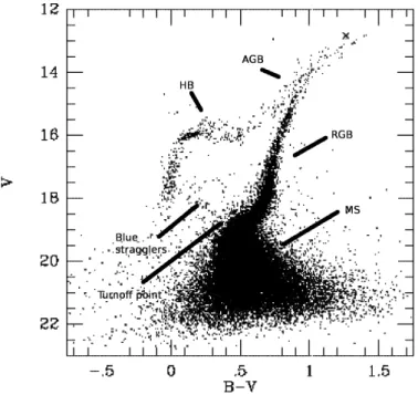
The evolution of stars can be understood using the Hertzsprung-Russell diagram (HRD). In an HRD, the luminosity of stars is plotted as a function of effective tem-perature. The HRD of our Milky Way consists of stars clustering around two main regions; one is the main sequence (MS) and one is the giant branch. Such an HRD were constructed with the Hipparcos satellite and can be seen in Figure 1.1. On the MS, the existence of a simple relation between the luminosity and effective temperature is due to one important parameter: the mass of the star. More massive stars are hotter and more luminous in the MS than stars with lower mass. The existence of the MS in due to the nuclear reactions that convert hydrogen into helium in the core of stars. The analog of HRD is the color-magnitude diagram (CMD). In this diagram, the horizontal axis contains a color (usually B−V, V−I) which relates to effective temperature, while the absolute magnitude is plotted on the vertical axis.
During pre-main-sequence evolution stars evolve from interstellar clouds due to grav-itational collapse. This phase is characterized by two time scales: the free-fall time scale at the beginning, and the Kelvin-Helmholtz time scale at later phases of contraction. Once the hydrogen fusion starts in the core of the star, the main-sequence evolution be-gins on the time scale of nuclear reactions. The main-sequence, and post-main-sequence evolution of a 1M⊙ mass and metal-poor1 star in the HRD is plotted in Figure 1.2.
The nuclear time scale is on the order of 1010 years. A low-mass star spends nearly 80−90% of its life on the MS. In this stage, the luminosity, radius and effective
tempera-ture increases slowly, but steadily. In the core of a low mass star the energy is created via 1
CHAPTER 1. INTRODUCTION 1.1. STELLAR EVOLUTION
Figure 1.1: The observational HRD constructed from the preliminary Hipparcos catalog
(Per-ryman et al., 1995). Left panel: The HRD of 8784 stars with less than 10% error in their
parallaxes (distance from Sun is smaller than 60−70 pc). Right panel: The HRD of 11125 stars
with errors between 10% and 20% in their parallaxes (distance from Sun is between 70 and
∼140 pc).
proton-proton (pp) cycles. The pp chain converts hydrogen to helium, while the mean molecular weight of the core increases. According to the ideal gas law, if the density or temperature of the core also increases, the gas pressure will not be enough to support the overlying regions of the star. Thus, the core must be compressed and, as a result, the density of the core increases and gravitational potential energy is released, which heats up the core. The pp chain reaction depends on temperature and increases as T4, which more than offsets the decrease of the mass fraction of hydrogen in the core. This results in an increase of the effective temperature and luminosity. During the MS evolution of low-mass stars the mass loss can be ignored, the mass of the star remains nearly constant. Eventually, as evolution continues, the hydrogen in the core will be depleted and the energy generation from pp chains stops. However, the core temperature is now so high, that the nuclear fusion becomes possible in a thick hydrogen-burning shell around a small, predominantly helium core. Now, the luminosity is being generated in this thick shell and eventually becomes larger than what was produced by the core during the core-burning phase. Some of this energy goes to expand the inner regions of the star, which results in a lower effective temperature with nearly constant luminosity (Figure 1.2). This hydrogen-burning shell continuously producing helium, thus the mass of the isothermal helium core
CHAPTER 1. INTRODUCTION 1.1. STELLAR EVOLUTION 1.0 2.0 3.0 3000 4000 5000 6000 log L/L ⊙ Teff (K) M=1.0M⊙ Z=0.003 MS HG RGB HB AGB post−AGB
Figure 1.2: Evolutionary track of a M=1M⊙ and Z=0.003 star on the HRD calculated with
the Single Star Evolution program developed by Hurley (2000). The stages labeled are the following in the order of evolution: 1. MS: main sequence, 2. HG: Hertzsprung gap, 3. RGB: red giant branch, 4. HB: horizontal branch, 5. AGB: asymptotic giant branch, 6. post-AGB:
evolution after the asymptotic giant branch.
increases.
This phase of evolutions ends when the isothermal core becomes so massive that it cannot support the pressure of material above it. This happens when the mass of the helium core reaches the Sch¨onberg-Chandrasekhar limit, which is around 10% of the star’s mass. When the mass of the core exceeds this limit it collapses on the Kelvin-Helmholtz time scale, and the star evolves very rapidly compared to the MS evolution. This occurs in the Hertzsprung gap (HG) on the HRD (Figure 1.2). The release of gravitational potential energy causes the core temperature to rise, and at the same time, the temperature and the density of the hydrogen-burning shell increase. This forces the star to expand rapidly. This continuous until the effective temperature reaches that of the Hayashi track (the path that a fully convective pre-main-sequence stars follows as it approaches the MS).
As the core continuous to contract, the energy production increases significantly from the hydrogen-burning shell. In this phase the evolution proceeds vertically in the HRD, until the star reaches the red giant branch (RGB), and significant mass loss starts by stellar winds. At this time, the core becomes strongly electron-degenerate and when the core temperature reaches 108 K to initiate the triple alpha process, the ensuing energy is explosive. This is the helium core flash. However, this energy release lasts for only a
CHAPTER 1. INTRODUCTION 1.1. STELLAR EVOLUTION
few seconds and never reaches the surface, because the overlying regions absorb it. This phase is the first time when significant amount of mass loss occurs from the surface. Due to the generated energy, the core becomes non-degenerate decreasing the density and temperature, and lowering the reaction rate of the triple alpha process. The star reaches the horizontal branch (HB) phase.
The hydrogen-burning shell continues to produce helium, and the mean molecular weight in the core increases to the point where the core starts to contract while the surface layers expand and cool. The energy required to increase the gravitational potential energy of the hydrogen-burning shell lowers the luminosity. During the phase of HB, almost all stars develop instabilities in their outer envelopes, resulting in periodic pulsations and variations in luminosity, effective temperature and radius.
At the end of the HB phase, the helium core becomes exhausted, just like the hydrogen core did at the end of the MS. As the core temperature further increases, a thick helium-burning shell develops above the core, but below the hydrogen-helium-burning shell. When the helium-burning shell starts to produce energy, the outer envelopes expand and cool, shutting down the hydrogen-burning shell. This shell will eventually reignite and the narrowing helium-burning shell begins to turn on and off periodically as the hydrogen-burning shell dumps helium into deeper regions. This phase is called the asymptotic giant branch (AGB). As the mass of the helium shell increases, it becomes degenerate, but when the temperature starts to increase, a helium shell flash occurs, driving the hydrogen shell outwards and cooling it down. Eventually the burning in the helium shell stops and the whole process starts again. The period between these pulses is a couple of hundreds of thousands of years for low-mass stars.
Mass loss becomes even more significant in the AGB phase, than before. Our under-standing of mass loss processes are poor, but it is suggested by many that it is linked to the helium shell flashes. Other proposed mechanisms come from the high luminosity and/or low surface gravity of these stars. Mass loss becomes more and more important as the star evolves in the AGB phase, because as the mass of the star decreases, the surface gravity decreases as well and the surface material becomes less tightly bound. The result of the mass loss is an increasement in the interstellar medium (ISM) and intracluster medium (ICM). Because of the low surface temperature of these stars and the stellar wind being rich in carbon and oxygen, dust production can be significant.
Eventually the mass loss becomes so strong and so much material will be lost, that the helium and hydrogen-burning shells shut down. The previously expanded shells becomes optically thin, revealing the dense core of the star, which purely consists carbon and oxygen. This central objects will then cool and become a white dwarf star, which is the final stage of the low-mass star evolution.
CHAPTER 1. INTRODUCTION 1.2. GLOBULAR CLUSTERS
1.2
Globular Clusters
A globular cluster is a spherical collection of stars that orbits a galaxy. These objects are tightly bound by gravity, which gives them their spherical shapes and relatively high stellar densities toward their centers. The Milky Way possesses about 160 known globular clusters. These star clusters play a very important role in astrophysics, mainly in stellar evolution.
Figure 1.3: Color-magnitude diagram of stars in M15. The photometry was taken by the WFPC2 camera on the Hubble Space Telescope (van der Marel et al., 2002).
It is believed that all stars in a globular cluster were produced at the same time, only 2−3 billion years after the Big Bang. These clusters are very metal-poor and one of the
oldest objects in the Universe. They are free of gas and dust and it is presumed that all of the gas and dust was long ago turned into stars, although some ICM still remains in some clusters, probably coming from stellar winds of AGB stars (see Section 1.3). Their size is usually couple of hundreds of light years across, and they consists of from several hundreds of thousands of stars to several million.
When the stars of a globular cluster are plotted on the HRD, nearly all of the stars fall upon a relatively well defined curve (Figure 1.3). This differs from the HRD of stars in the Milky Way (Figure 1.1), which consists of stars of different ages and origins. The shape of the curve for a globular cluster is characteristic of stars that were formed at approximately the same time with nearly the same metallicity, differing only in their initial mass. For a population of stars with the same age, as the population ages, the more massive stars will begin to leave the MS, which results in the turnoff point on the
CHAPTER 1. INTRODUCTION 1.2. GLOBULAR CLUSTERS
MS moving to lower luminosities. Such an evolutionary trend can be used to estimate the age of a stellar population, because the turn off occurs when nearly all the central fuel is gone in the core of the star. Blue stragglers are stars that are hotter and bluer than other cluster stars having the same luminosity. These stars appear to be merging binary stars.
Two clusters with the same metallicity have to have two very similar HRDs, but observation show that the HB can be very different even in this case.
1.2.1
The Second Parameter Problem
The well-known second parameter problem in globular clusters (Sandage & Wildey, 1967), in which a parameter other than metallicity, affects the morphology of the hori-zontal branch, remains unresolved. Metallicity, as first noted by Sandage & Wallerstein (1960), remains the principal parameter, but pairs of clusters, with the same metallic-ity, display quite different horizontal branch morphologies thus challenging the canonical models of stellar evolution and leading to the need for a ‘Second Parameter’. Cluster ages have been examined in many studies (Searle & Zinn, 1978; Lee et al., 1994; Stetson et al., 1996; Lee & Carney, 1999; Sarajedini, 1997; Sarajedini et al., 1997) and in addition, many other suggestions for the ‘second parameter(s)’ have been proposed, including: to-tal cluster mass; stellar environment (and possibly free-floating planets); primordial He abundance; post-mixing surface helium abundance; CNO abundance; stellar rotation; and mass loss (Catelan, 2000; Catelan et al., 2001; Sills & Pinsonneault, 2000; Soker et al., 2001; Sweigart, 1997; Buonanno et al., 1993; Peterson et al., 1995; Buonanno et al., 1998; Recio-Blanco et al., 2006). Many authors (Vandenberg et al., 1990; Lee et al., 1994; Catelan, 2000) have proposed that more than one second parameter may exist in addi-tion to age. One parameter may be mass loss which, as Catelan (2000) notes, remains an ‘untested second-parameter candidate’.
An example of paired second-parameter clusters is M15 and M92 ([Fe/H]=−2.26 and −2.28 respectively). Although the metallicities of these two clusters are the same (Sneden
et al., 2000), their horizontal branches differ (Buonanno et al., 1985). M92 has a brighter (by about one magnitude) and redder blue HB extension than M15. The color magnitude diagrams of this pair were examined in detail by Cho & Lee (2007). They found that the difference in the HB morphology between the two is probably not a result of deep mixing in their red giant branch sequences, because no significant ‘extra stars’ were found in their observed RGB luminosity functions compared to the theoretical RGB luminosity functions. Sneden et al. (2000) found that Si, Ca, Ti, and Na abundance ratios of the red giants are nearly the same in both clusters, only the [Ba/Ca] ratio shows a large scatter and the mean value in M15 is twice that found in M92. These studies eliminate deep mixing and subtle abundance variations as possible second parameters. Mass loss
CHAPTER 1. INTRODUCTION 1.2. GLOBULAR CLUSTERS
is examined in this thesis in Section 4.3. Detailed observations of red giant stars in M15 are contained in M´esz´aros et al. (2008), but the comparison between M15 and M92 is described in M´esz´aros et al. (2009a,b).
Figure 1.4: Color-magnitude diagram of stars in the second-parameter clusters M13 and M3. Note the significant difference between the HB of these two clusters. The photometry was taken
by the Hubble Space Telescope (Ferraro et al., 1997).
M13 ([Fe/H]=−1.54) is one of the most studied second-parameter globular clusters.
M13 and M3 are almost identical in most respects (metallicity, age, chemical composi-tion), but there are dramatic differences in both the HB and blue straggler populations (Figure 1.4). Analysis of both clusters’ CMDs (Ferraro et al., 1997) with the Hubble Space Telescope revealed that neither age nor cluster density, two popular second-parameter candidates, is likely to be responsible for the differences in these clusters. From the analysis of high-resolution, high signal-to-noise ratio spectra of six RGB stars in M3 and three in M13, Cavallo & Nagar (2000) found that the [Al/Fe] and [Na/Fe] abundances increase toward the tip of the RGB. They concluded that the data for both clusters are consistent with deep mixing as a second parameter. Later, Johnson et al. (2005), from medium−resolution spectra of more than 200 stars in M3 and M13, concurred that
deep mixing is the best candidate for second parameter in this pair of clusters. Caloi & D’Antona (2005) also examined the second-parameter problem in M3 and M13 in detail and proposed that the overall difference between M3 and M13 CMD morphologies is due
CHAPTER 1. INTRODUCTION 1.3. MASS LOSS
to the different helium content. Since M13 does not have a red clump in its horizontal branch they suggested that it represents an extreme case of self-enrichment of helium, which might come from the massive asymptotic giant branch stars (AGB) in the first
∼100 Myr of the cluster life.
A multivariate study of the CMDs for 54 globular clusters was carried out by Recio-Blanco et al. (2006) from Hubble Space Telescope photometry to quantify the parameter dependencies of HB morphology. They found that the total cluster luminosity (therefore the total mass) has the largest impact on the HB morphology, and as Caloi & D’Antona (2005) speculated, there may be enrichment of helium from an earlier population of stars. D’Antona et al. (2002) modeled the evolution of globular cluster stars and showed that different choices of mass−loss rate affect the distribution of stars on the HB.
1.3
Mass Loss
Although stellar evolution theory predicts that low-mass Population II stars ascending the red giant branch (RGB) for the first time must lose mass (Renzini, 1981; Sweigart et al., 1990), few observations have identified the ongoing mass loss process. Evidence from the period-luminosity relation for RR Lyrae stars suggests that the luminosity variations can be accommodated theoretically if mass loss ∼0.2−0.4M⊙ has occurred (Fusi Pecci
et al., 1993; Christy, 1966). Iben & Rood (1970) conjectured that mass loss on the RGB may increase with metallicity in order to account for colors on the horizontal branch.
For stellar evolution calculations, the mass loss rate from late-type giants is frequently described by “Reimers’ law” (Reimers, 1975, 1977) given as ˙M[M⊙yr−1] =η×L∗×R∗/M∗,
where L∗, R∗, and M∗ are the stellar luminosity, radius, and mass in solar units, and η
is a fitting parameter equal to 4×10⁻¹³. This approximation is based on a handful of
luminous Population I stars.
Schr¨oder & Cuntz (2005) offered another semi-empirical relation for the mass loss rate from cool stars by assuming a wave-driven wind and introducing gravity and ef-fective temperature into the formulation. They found consistency with calculations of evolutionary models for abundances as low as [Fe/H]=−1.27 although metallicity does not enter as a parameter in their formulation.
1.3.1
Direct Evidence
Direct observations of the ongoing mass loss process in globular clusters only became possible in the past decade using high resolution spectroscopy and infrared imaging from space.
Circumstellar CO emission in M-type irregular and semi-regular asymptotic giant branch (AGB)-variables implies mass loss rates on the AGB ∼ 10−7 −10−8 M⊙ yr−1
CHAPTER 1. INTRODUCTION 1.3. MASS LOSS
(Olofsson et al., 2002). Indirect evidence of mass loss processes would be detection of an intracluster medium. These efforts have been marginally successful. Diffuse gas (< 1 M⊙) was suggested in NGC 2808 through the detection of 21−cm H line emission
(Faulkner et al., 1991), but has remained unconfirmed. Ionized intracluster gas was found in the globular cluster 47 Tucanae by measuring the radio dispersion of millisecond pulsars in the cluster (Freire et al., 2001). The central electron density was derived (ne = 0.067 ±0.0015 cm−3) and found to be two orders of magnitude higher than the
ISM in the vicinity of 47 Tuc (Taylor & Cordes, 1993). Freire et al. (2001) determined the electron density in M15 using four millisecond pulsars to be higher (ne ∼0.2 cm−3)
than in 47 Tuc.
Indirect evidence of mass loss processes comes also from infrared observations. Origlia et al. (2002) using ISOCAM images found a mid-IR excess associated with giants in sev-eral globular clusters and attributed to dusty circumstellar envelopes. The first detection of intracluster dust in M15 was made by Evans et al. (2003) from the analysis of far infrared imaging data obtained with the ISO instrument ISOPHOT. van Loon et al. (2006) also presented a tentative detection of 0.3M⊙ of neutral hydrogen in M15. Smith
et al. (1995) placed an upper limit of 0.4 M⊙ for the molecular gas in M15 from CO
observations with the 15-m James Clerk Maxwell Telescope on Mauna Kea. Using the
Spitzer Space Telescope, Boyer et al. (2006) detected a population of dusty red giants near the center of M15. Observations with the Multiband Imaging Photometer forSpitzer
(MIPS) also revealed the intracluster medium discovered by Evans et al. (2003) near the core of the globular cluster. As Origlia et al. (2002) noted, the infrared detections may only be tracing the outflowing gas and may not be related to the driving mechanisms for the wind. More recently Origlia et al. (2007) identified dusty RGB stars in 47 Tuc and derived an empirical mass loss law for Population II stars. Mass loss rates derived from these observations showed that the mass loss increases with luminosity and possibly it is episodic.
1.3.2
Spectroscopic Studies
High resolution stellar spectroscopy allows the direct detection of mass outflow from the red giants themselves. Emission in the wings of Hα lines in the spectra of globular cluster red giants was first described in detail by Cohen (1976). Later observations revealed that emission in Hαis common in globular clusters and night-to-night variations can occur (Mallia & Pagel, 1981; Peterson, 1981, 1982; Cacciari & Freeman, 1983; Gratton et al., 1984). These studies have shown that most of the stars brighter than log (L/L⊙)≈
2.7 exhibit Hα emission wings.
The emission itself is likely not a direct indicator of mass loss, because emission can arise from an optically thick stellar chromosphere surrounding the star (Dupree et al.,
CHAPTER 1. INTRODUCTION 1.4. MODELS FOR MASS LOSS
1984). Variation of the strength of emission can also be affected by stellar pulsation (Smith & Dupree, 1988). Better mass flow indicators in the optical are the line coreshifts or asymmetries of the Hα or Ca II H&K profiles and emission features. Red giants in globular clusters (M22 and Omega Centauri) were found to have velocity shifts less than 14 km s−1 in the cores of Hα relative to the photospheric lines (Bates et al., 1990, 1993). These results were similar to metal-poor field giants, where only giants brighter than MV =−1.7 have emission wings and the line shifts were < 9 km s−1 (Smith & Dupree,
1988) indicating very slow outflows and inflows in the chromosphere.
For globular clusters, Lyons et al. (1996) discussed the Hαand Na I D line profiles for a sample of 63 RGB stars in M4, M13, M22, M55, and ω Cen. The coreshifts were less than 10 km s−1, much smaller than the escape velocity from the stellar atmosphere at 2R
∗
(≈50−70 km s−1). Dupree et al. (1994) studied 2 RGB stars in NGC 6752 and found that the CaIIK and Hαcoreshifts were also low (less than 10 km s−1). However, asymmetries in the Mg II lines showed a stellar wind with a velocity of ≈ 150 km s−1, indicative of a strong outflow in cluster giants and metal-poor field stars (Dupree et al., 1994, 2007; Smith & Dupree, 1988). However, Mg II lines are formed higher in the atmosphere than Hα and CaIIK, which suggests that the stellar wind becomes detectable near the top of the chromosphere. These Mg II lines showed strong outflow velocities (≈ 150 km s−1).
Also, high outflow velocities, (30−140 km s−1), were found in the He I λ10830 absorption
line of metal-poor red giant stars of which 6 are in M13 (Dupree et al., 1992; Smith et al., 2004; Dupree et al., 2009). These outflow velocities are frequently higher than the central escape velocities from globular clusters, namely 20−70 km s−1 (McLaughlin & van der Marel, 2005).
A detailed study was carried out by Cacciari et al. (2004), who observed 137 red giant stars in NGC 2808. Most of the stars brighter than log (L/L⊙) = 2.5 clearly
showed emission wings in Hα . The velocity shift of the Hα line core compared to the photosphere is less than ≈9 km s−1 . Outward motions were also found in both Na I D
and CaII K profiles. Another detailed study of Hα line and CaIIK profiles were carried out with the Hectochelle on the MMT at a resolution of 34,000 by M´esz´aros et al. (2008, 2009a) in M13, M15 and M92. These results are discussed in this thesis in Section 2, 3 and 4.
1.4
Models for Mass Loss
Semi-empirical modeling of spectral features to derive mass loss rates are quite rare in the literature. These kind of studies are the only ones, where the mass loss rate can be determined directly from the spectrum of stars.
In order to evaluate the mass flow, detailed non-LTE modeling with semi-empirical atmospheres is necessary to reproduce the optical line profiles and infer the mass loss rates
CHAPTER 1. INTRODUCTION 1.5. GOALS
from the stars. Such non-LTE modeling was first carried out by Dupree et al. (1984). They showed that the emission wings of the Hα line found in metal-deficient giant stars can arise naturally from an extended, static chromosphere, and emission asymmetry and shifts in the Hα core indicate mass loss. Spherical models with expanding atmospheres suggested the mass loss rates are less than 2×10⁻⁹ M
⊙ yr−1 a value which is less than
predicted by the Reimer’s relationship.
McDonald & van Loon (2007) calculated mass loss rates of two stars in M15 by modeling the Hα and Ca II K lines with simple LTE approximations. They found mass loss rates of several times 10−8 and 10−7M
⊙ yr−1, but the use of LTE models for a
chromosphere can not be considered reliable.
Mauas et al. (2006) computed semi-empirical Hα and CaII K profiles for 5 RGB stars in NGC 2808 including non-LTE effects in spherical coordinates. Their line profiles fit the observations when an outward velocity field is included in the model chromosphere, in agreement with previous calculations (Dupree et al., 1984). The derived mass loss rates exhibited a large range around 10−9 M
⊙ yr−1. Outflow velocities from 10 km s−1
up to 80 km s−1 were needed by Mauas et al. (2006) in order to match the observed line profiles.
M´esz´aros et al. (2009b) presented chromospheric model calculations of the Hα line for selected RGB and AGB stars in M13, M15, and M92 to derive mass loss rates. These results are discussed in Section 5.
1.5
Goals
This thesis discusses high-resolution spectroscopy of the Hα and CaII H&K lines of red giant stars in M15 ([Fe/H]=−2.26), M13 ([Fe/H]=−1.54) and M92 ([Fe/H]=−2.28)
(M´esz´aros et al., 2008, 2009a). The deep sample of M13, M15, and M92 giants offers a good comparison to other studies of the more metal rich cluster NGC 2808 ([Fe/H]=−1.15)
(Cacciari et al., 2004). The high resolution spectrograph Hectochelle gives an excellent opportunity of determine the line bisectors of the Hα line and explore the mass motions in the chromosphere of these stars.
Detailed study of these four clusters allows the examination of a possible dependence between the average cluster metallicity and characteristics of Hα and Ca II K emission, and diagnostics of mass outflow. Observations with the same instrument of the second-parameter pair M15 and M92 offer a good comparison to examine mass loss as a possible second parameter.
I also selected a sample of giant stars to model whose spectra have been obtained previ-ously with Hectochelle (M´esz´aros et al., 2008, 2009a). They span a factor of 5 in metallic-ity (from [Fe/H]=−1.54 to−2.28) and a factor of 6 in luminosity [from log (L/L⊙) =2.57
The observation technique, target selection and data reduction is explained in Section 2. Section 3 describes the line statistics, radial velocity measurements and the line bisector characteristics. Section 4 discusses the appearance of Hα and Ca II K emission and bisectors on the CMD. Section 5 contains the details of the non-LTE models in both the static and expanding versions, and compares the calculations with Hα line profiles, and the construction of a mass loss relation and its dependence on temperature, luminosity, and abundance.
Chapter 2
Observations
In this Chapter, I describe how the observations were obtained during 2005 and 2006. The first section contains a brief summary on the Hectochelle spectrograph and the target selection criteria. The second section explains the steps of data reduction in IRAF1.
2.1
Target Selection
Observations of a total of 297 red giant stars in M13, M15 and M92 were obtained in 2005 May, 2006 May, and 2006 October with the Hectochelle on the Multi Mirror Telescope (MMT) (Szentgyorgyi et al., 1998). The Hectochelle is a fiber-fed, bench mounted echelle spectrograph, which operates on the MMT in wide field mode covering 1 degree on the sky. Hectochelle uses 240 fibers and each of them subtends ∼1.5 arcsec.
These fibers can be placed∼2 arcsec apart across the field of view, and can be positioned
with an accuracy of 25 µm. Hectochelle operates in a is a single-order mode, when a spectral order is isolated with a bandpass filter, giving∼150 ˚A width in each order. This
way, in optimal case, 240 stars can be observed at the same time having the same spectral range for each star with a resolution about 34,000 in each filter. The CCDs positioned in the focal plane are cooled to −120 Celsius with liquid nitrogen and consist of a pair of 2k × 4.5k devices with 13.5µm pixels.
The apparent diameter of M15 is only ∼ 12 arc minutes, so that about 50−60 red
giants could be measured in each configuration. The apparent diameter of M13 is ∼15
arc minutes, and about 60−70 red giants in the globular cluster could be selected in the
field of view. The apparent diameter of M92 is smaller, and only 30−40 stars could be
measured with one configuration. Observations of a total of 110 red giant stars in M15 were made in 2005 May, 2006 May, and 2006 October, in four different fiber configurations. Two separate input fiber configurations for different stars were made for M13 and M92. A total of 123 different red giant stars in M13 and 64 red giants in M92 were observed in
1
CHAPTER 2. OBSERVATIONS 2.1. TARGET SELECTION
2006 March and 2006 May.
12 13 14 15 16 0.6 0.8 1.0 1.2 1.4 1.6 V B−V
M13
12 13 14 15 16 0.6 0.8 1.0 1.2 1.4 1.6 V B−VM15
12 13 14 15 16 0.6 0.8 1.0 1.2 1.4 V B−VM92
Figure 2.1: Color-magnitude diagram for all stars observed in M13, M15, and M92. The solid line shows the fiducial curve of the RGB; the dashed line shows the fiducial curve of the AGB for M13 and M92 taken from observations of Sandage (1970), for M15 taken from observations of
Durrell&Harris (1993). The absolute magnitudes were calculated using the apparent distance
modulus(m−M)V = 14.48for M13,(m−M)V = 15.37for M15, and(m−M)V = 14.64for
M92 from Harris (1996).
The requirement that fibers cannot be placed closer than 2 arcsec apart further con-strains the target selection, especially near the cluster’s core. To ensure that large number of objects are observed and reduce the possibility of blends, stars from the outer regions of the clusters were mainly selected. In addition, I wanted to search for variability which led to multiple visits for many targets over the 17 month span in M15, thus several stars were chosen multiple times. Software (xfitfibs2) has been developed at CfA to optimize the fiber configuration with specified priorities and requirements.
Targets brighter than 15.5 magnitude with a high probability (>95%) of membership were chosen from the catalog of Cudworth (1976) for M13 and M15, and from Cudworth & Monet (1979) for M92 to provide smooth coverage of the RGB and AGB within the constraint of the fiber placement on the sky. The color magnitude diagram (CMD) of the observed cluster members can be seen in Figure 2.1 and they are listed in Appendix Table 7.1 for M15, in Appendix Table 7.2 for M13, and in Appendix Table 7.3 for M92. Coordinates of the stars were taken from the 2MASS catalog (Skrutskie et al., 2006) and used to position the fibers. Additional targets from Cudworth’s list with lower
2
CHAPTER 2. OBSERVATIONS 2.1. TARGET SELECTION
Table 2.1. Hectochelle Observations of M13, M15, and M92 Date Total exp. Wavelength Filter Name Number of
(UT) (s) (˚A) Observed Stars
2006 March 14 (M13, Field 1) 3×2400 6475−6630 OB25 70 2006 March 16 (M13, Field 1) 3×2400 3910−3990 Ca41 70 2006 March 16 (M13, Field 1) 1×2400 5150−5300 RV31 65 2006 May 10 (M13, Field 2) 3×2400 6475−6630 OB25 70 2006 May 10 (M13, Field 2) 3×2400 3910−3990 Ca41 63 2006 May 10 (M13, Field 2) 1×2400 5150−5300 RV31 65 2005 May 22 (M15, Field 1) 3×1200 6485−6575 OB25 53 2005 May 23 (M15, Field 1) 3×1200 3910−3990 Ca41 53 2006 May 11 (M15, Field 2) 3×2100 6475−6630 OB25 54 2006 October 4 (M15, Field 3) 3×2100 6475−6630 OB25 58 2006 October 7 (M15, Field 4) 3×2100 6475−6630 OB25 50 2006 May 7 (M92, Field 1) 3×2400 6475−6630 OB25 42 2006 May 7 (M92, Field 1) 3×1800 5150−5300 RV31 40 2006 May 8 (M92, Field 1) 3×2400 3910−3990 Ca41 41 2006 May 9 (M92, Field 2) 3×1800 6475−6630 OB25 36 2006 May 9 (M92, Field 2) 3×2400 3910−3990 Ca41 36
membership probability and field targets from the 2MASS catalog were included for M15.
During the first observations in 2005 few fibers were positioned on the sky, because it was believed that only 20−30 apertures are enough to monitor the sky intensity in the field
of view. After the first reductions it turned out that many more sky fibers are necessary (see next Section 2.2), thus in later observations additional field targets and stars with low membership probability were neglected, and the remaining fibers (∼ 150−200) were
positioned on the sky. The sky fibers were equally distributed in the observed field to cover a large area around the clusters omitting the cluster core. Exposure times varied between 20 and 40 minutes, which gave a S/N∼15 for the faintest objects. 40 minute
exposure times were crucial for the Ca41 filter, because the measured flux is very small for red giant stars in the blue region of the spectrum.
Since Hectochelle is a single-order instrument, three orders were selected with order-separating filters: OB25 (Hα, region used for analysis λλ 6475−6630)3, Ca41 (Ca II K region used for analysis λλ 3910−3990), and RV31 (region used for analysisλλ 5150−
5300). OB25 and Ca41 filters gave 155 ˚A centered on the principal spectral features in Hα and 80 ˚A in Ca II H&K. RV31 filter was used to determine accurate radial velocity of the stars in M13 and M92. The spectral resolution was about 34,000 as measured by the FWHM of the ThAr emission lines in the comparison lamp. Exposures in each of the three orders are summarized in Table 2.1. A raw CCD image of Hectochelle with the Ob25 filter can be seen in Figure 2.2.
Bias and quartz lamps for the flat correction were obtained each day. In early ob-servations (2005), exposures with the ThAr comparison lamp were obtained during the
CHAPTER 2. OBSERVATIONS 2.2. DATA REDUCTION
Figure 2.2: Raw CCD image of Hectochelle with the OB25 filter taken on 2006 March 14 from selected red giants in M13. There are 240 apertures in the CCD, but only the ones with bright
stars are visible here.
afternoon with exposure times of 900 sec. As the observation techniques evolved, expo-sures with the ThAr lamp were taken with exposure times of 150 sec before and after every observation during the night to determine the wavelength solution. The number of objects observed changed slightly between observations, because fiber positions need to be reconfigured when targets pass the meridian.
In the 2005 May spectra of Hα in M15, the filter’s central wavelength was offset by∼
80 ˚A placing the Hαline near the long wavelength end of the CCD. Fluxes at wavelengths shorter than Hα were abnormally low, because the grating was so far off the blaze angle. The wavelength regions spanned by the OB25 filter differed between the 2005 and 2006 observations; however both contained the Hα line and photospheric lines.
2.2
Data Reduction
Data reduction was done using standard IRAF spectroscopic packages. The IRAF package ccdproc performed the trimming and the overscan correction and made the bad pixel mask using a template created for the CCD camera of Hectochelle. The trimming correction was necessary because a swap of an I/O card in chelle electronics caused an additional pixel at the beginning of each row. The overscan correction was done to target and bias images as well to monitor possible changes in pixel count with time.
CHAPTER 2. OBSERVATIONS 2.2. DATA REDUCTION
The overscanned and averaged bias image was then subtracted from every spectrum. Correcting with the dark images was not necessary because even in the 40 minute dark exposures the intensity was very low [3 −4 analog digital units (ADU) per pixel].
To find and trace the apertures, ten flat images were taken with the continuum lamp of 10 seconds exposure time each. The focal plane of Hectochelle consists of a mosaic of 2 CCDs that are slightly misaligned. The aperture finding algorithm fails near the crack between the two CCDs, so manually editing the apertures and reordering them was necessary. Some apertures were deleted from the edges of the CCD and a total of 240 orders was extracted.
To correct for the pixel-to-pixel variations, the averaged continuum flat exposures for each configuration were fitted with a 21st order spline function (using the IRAF task apflatten) and used to divide the corresponding object spectra by the normalized flat. A region 13−pixels wide was carefully selected for the aperture extraction, because
apertures are close to each other and scattered light from a bright star can affect the neighboring apertures.
Wavelength standards, using ThAr hollow cathode lamps were taken to define the wavelength scale; each ThAr image obtained in 2005 had 900 seconds of exposure time and was taken at the beginning of the night. For observations taken in 2006, the 150 seconds of exposure time ThAr images taken before and after every scientific exposure were used for determining the wavelength solution. This allowed to eliminate small wavelength shifts coming from the different fiber placements during the night. I identified 15 − 20 strong ThAr emission lines in the first aperture, then propagated these identifications to every other aperture manually to check the accuracy of the fit. During the calibration the rms of the wavelength fit had to be between 0.01−0.002 ˚A to reach the theoretical resolution
of the spectrograph. If the error of the fit is larger than this, it will be comparable to the expected width of the ThAr features (0.1 − 0.2 ˚A) and increase the error of the
wavelength solution.
The continuum flat images were used to correct the throughput for each aperture us-ing a region close to the CCD center containus-ing 5 − 7 neighboring fibers. An average of
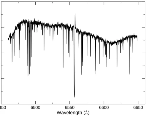
the selected continuum flat apertures was taken and divided into all other apertures in the same exposure and was used to correct the vignetting and fiber-to-fiber throughput devi-ation. An example of a extracted, wavelength calibrated spectrum after the throughtput correction can be seen in Figure 2.3.
The extracted spectra also contain sky background which had to be subtracted. Some of the sky apertures showed weak Hα and other photospheric lines suggesting very faint stars in those positions. Also very bright stars can cause scattered light in the neighboring apertures on the CCD, but this becomes visible only if the aperture has more than 8000 −10000 ADUs per pixel. The brightest stars reached 10000 ADUs per pixel in the
CHAPTER 2. OBSERVATIONS 2.2. DATA REDUCTION 2000 4000 6000 8000 6450 6500 6550 6600 6650 ADU Wavelength (Å)
Figure 2.3: Example of a Hαspectrum taken on 2006 March 14 after all reductions, but before sky subtraction and continuum normalization.
Every sky aperture was checked carefully and those where faint stars or scattered light were found were discarded. A median filtered sky was used for the subtraction, but sky subtracted skies frequently contained additional counts, which changed aperture by aperture and by wavelength. In Figure 2.4, a sample of sky intensity versus wave-length and aperture is plotted for the Hα filter. Between aperture numbers 100 and 150, especially at longer wavelengths, the apertures have higher intensity. The dark images did not show high intensity features and the intensity pattern in Figure 2.4 is currently not understood. To subtract the sky, the images were divided into 3 different aperture sections, and the sky subtraction was done with the following method. In the first and third segments (corresponding to aperture numbers 0−100 and 150−240), the intensity
appears constant as a function of aperture number and wavelength so the median filtered spectrum could be used for subtraction. The middle region spanned aperture numbers 101 to 149, in this region the sky was subtracted from every target aperture using the average of 3 closest sky apertures on the CCD itself.
Continuum normalization was done with the IRAF task continuum. A one dimen-sional, low order Chebyshev function was fit to the continuum of each spectra individually to produce a normalized spectrum. The normalization of the spectra obtained with the OB25 and RV31 filter is well determined, because the continuum is visible and deep lines like the Hα line were omitted from the fit. Continuum normalization is challenging in the Ca41 filter, because hundreds of absorbing lines depress the continuum
substan-260 220 180 140 100
Aperture
Wavelength (
Å
)
250 200 150 100 50 0 6620 6600 6580 6560 6540 6520 6500 6480Figure 2.4: Variations in the intensity of the sky apertures in the Hαfilter. Dark area indicates the highest count level. See scale at right. An anomalous intensity pattern occurs, which is currently not understood. Special extraction patterns were used for the sky fibers (see text).
tially. Here, also a low order Chebyschev function was used to fit and normalize the local continuum away from the strong CaII lines.
Chapter 3
Line Statistics
In the first section of this chapter I describe how radial velocity measurements were done, which is important to determine which stars are cluster members. In the second section I explain how emission features were identified in the Hαand CaIIK spectrum. In the third section I briefly review the position of stars with Hαemission on the CMD. The fourth section describes the Hαline bisector and its determination, which shows motions in the atmosphere, while the last section explains the CaII K emission characteristics.
3.1
Radial Velocity Measurements
Radial velocity measurements use the Doppler-effect. The Doppler-effect results in either a redshift, or a blueshift of spectral features of a receeding or an approching light source. The radial velocity of a star can be measured accurately by taking a high-resolution spectrum and comparing the measured wavelengths of known spectral lines to wavelengths from laboratory (rest-frame) measurements. By convention, a positive radial velocity indicates that the object is receding, a negative radial velocity means that the object is approaching. If spectral features are dominating the spectrum of a star, the cross-correlation is the widely accepted method to measure the radial velocity.
The cross-correlation is a measure of similarity of two spectra as a function of a time-lag applied to one of them. The definition of cross-correlation is:
f ⋆ g =
∞ Z −∞
f(τ)g(t+τ)dτ (3.1)
Consider two functions f andg that differ only by a shift along the x-axis. The equation slides the g function along the x-axis, calculating the integral of their product for each possible amount of sliding. When the two functions match, the value off ⋆gis maximized.
CHAPTER 3. LINE STATISTICS 3.1. RADIAL VELOCITY MEASUREMENTS
The definition of cross-correlation can be given by using Fourier transforms:
F (f ⋆ g) = F∗(ν)G(ν) (3.2)
where F denotes the Fourier transform, F∗(ν) denotes the complex conjugate of F(ν) = F [f(τ)]. In this casef ⋆gcan be obtained by the inverse Fourier transformF−1[F(ν)G(ν)].
For discrete and two real valued functions, f and g, the cross-correlation is defined as: (f ⋆ g)[n] =
∞ X
m=−∞
f[m]g[n+m] (3.3)
In the case of radial velocity measurement both f and g are spectra, where f is the observed, g is the template spectrum. τ represents the small ∆λ, which we use to shift the template. The position of the peak of the cross-correlation function gives the value of radial velocity. It is important to select templates similar to the observed spectra, otherwise the cross-correlation function will not have a well-determined peak.
3.1.1
M15
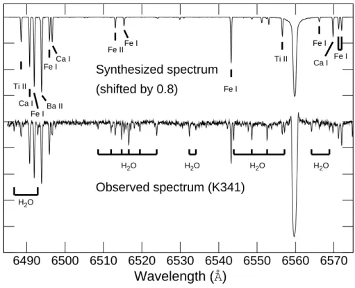
To measure accurate radial velocities I chose the cross-correlation method using the IRAF taskxcsao. Using the ATLAS (Kurucz, 1993) code, I synthesized the spectrum of a red giant star, K341, in M15. This is a bright star with a high quality spectrum, thus the comparison between the observed and modeled spectrum is optimum. The physical pa-rameters of the template spectrum were the following: Teff = 4275 K, log g = 0.45, vturb = 0 km s−1, vmacro = 0 km s−1, [Fe/H]=−2.45, [Na/Fe]=0.01, [Si/Fe]=0.4, [Ca/Fe]=0.56, [Ti/Fe]=0.57, [Ba/Fe]=0.2 (Sneden et al., 2000). This spectrum is com-puted in LTE and a chromosphere was not included in the atmospheric model, thus it only contains absorption features. The comparison between the template in our cross-correlation and the observed Hectochelle spectrum can be seen in Figure 3.1. Radial velocity measurements were only possible using the OB25 filter, because observations with the RV31 filter were not obtained for stars in M15. All determined radial velocities are corrected to the solar system barycenter.
The region selected for the cross-correlation spanned 6480 ˚A to 6545 ˚A purposely omitting the Hα line. The telluric and photospheric lines were identified using the syn-thesized spectrum of K341. In this region there are many telluric lines of water vapor. These lines appear in the cross-correlation function profile as an additional peak, well separated from the cluster velocity, and so the measured stellar radial velocity is not affected. To verify our radial velocities, I cross-correlated a narrow regionλλ6480−6500
where no strong telluric lines are found. Cross-correlating this narrow region results in the same radial velocity as from the broader window, but with a larger (1−2 km s−1)
CHAPTER 3. LINE STATISTICS 3.1. RADIAL VELOCITY MEASUREMENTS 0 0.2 0.4 0.6 0.8 1.0 1.2 1.4 1.6 1.8 6490 6500 6510 6520 6530 6540 6550 6560 6570
Wavelength (
Å
)
Relative Flux
Synthesized spectrum (shifted by 0.8) Observed spectrum (K341) H2O H2O H2O H2O Ti II Ca I Fe I H2O Ba II Fe I Ca I Fe IIFe I Fe I Ti II Fe I Ca I Fe IFigure 3.1: Kurucz synthesized spectrum shifted by 0.8 in relative flux and corrected for the star’s radial velocity shown above the observed spectrum of K341 in M15. Atmospheric water
vapor and other elements are marked.
error.
The Hαspectra of our targets were also cross-correlated against several hundred spec-tra calculated by Coelho et al. (2005) covering temperatures between 3500 and 7000 K and metallicities between [Fe/H]=−2.5 and +0.5. These velocities from the Coelho
spec-tra agreed within 1 to 2 km s−1 with our earlier determination using only the K341 template, because the same photospheric Fe and Ti absorption lines can be found in all the spectra.
There is good agreement between our radial velocities from the 2005 data and those of Gebhardt et al. (1997) and Peterson et al. (1989) (see Figure 3.2, top panels). Gebhardt et al. (1997) used an Imaging Fabry-Perot Spectrophotometer with the Sub-arcsecond Imaging Spectrograph on the Canada-France-Hawaii Telescope and observed 1534 stars in M15 with velocity errors between 0.5 and 10 km s−1. Peterson et al. (1989) used echelle spectrographs on the MMT, the 1.5 m Tillinghast reflector of the Whipple Observatory on Mount Hopkins, and the 4−m telescope of Kitt Peak National Observatory. Peterson
et al. (1989) quote an average error of 1 km s−1, but the stars in common with our sample have larger errors (1−2 km s−1).
However the Hectochelle velocities from 2006 display a systematic offset from the 2005 measurements of the same stars (see Figure 3.2, lower panels). This offset amounts to +1.9 ±0.5 km s−1 and +0.9 ±0.5 km s−1 for 2006 May and Oct 2006 respectively,
CHAPTER 3. LINE STATISTICS 3.1. RADIAL VELOCITY MEASUREMENTS -120 -110 -100 -90 -120 -110 -100 -90 vrad, 1 (km s-1) vgeb (km s -1 )
M15
-120 -110 -100 -90 -120 -110 -100 -90 vrad, 1 (km s-1) vpet (km s -1 )M15
-120 -110 -100 -90 -120 -110 -100 -90 vrad, 1 (km s-1) vrad, 2 (km s -1 )M15
-120 -110 -100 -90 -120 -110 -100 -90 vrad, 1 (km s-1) vrad, 3 (km s -1 )M15
Figure 3.2: Top left: Radial velocities measured on 2005 May 22 (vrad,1) for the same stars
observed by Gebhardt et al. (1997) (vgeb) in M15. Top right: Radial velocities measured on
2005 May 22 (vrad,1) for the same stars observed by Peterson et al. (1989) (vpet). There is good agreement between observations taken on 2005 May 22 and observations for the same stars from Gebhardt et al. (1997) and Peterson et al. (1989). Lower left: Radial velocity measured
with Hectochelle for the same stars observed on 2005 May 22 (vrad,1) compared to 2006 May
11 (vrad,2). The velocity offset between 2006 May 11 and 2005 May 22 is+1.9 ±0.5 km s−1
. Lower right: Radial velocities for the same stars measured with Hectochelle on 2005 May
22 (vrad,1) compared to 2006 October 4 (vrad,3). The velocity offset between 2006 October 4
and 2005 May 22 is+0.9 ±0.5km s−1. The dashed line marks a 1:1 relation. The offsets are
applied to our radial velocities for the 2006 May and 2006 October spectra.
and the data in Appendix Table 7.7 were corrected for this systematic offset. The radial velocities of the sky emission lines show the same effect. In 2005, all of the sky emission lines were at 0 km s−1 and in 2006 May were at−2 km s−1, yet the wavelength calibration of the 2006 data appears to be as accurate as 2005. The source of this offset comes from using the ThAr comparison lamp obtained during the afternoon and not before and after the scientific exposures. The telescope is at zenith for the afternoon calibration lamps, however the observed clusters are at a very different position on the sky. When the telescope moves, the position of fibers changes in their chamber, which introduces small linear 1−2km s−1 shifts in the spectra. The amount of the offset is small, and does not affect determination of cluster membership. The average cluster radial velocity was calculated using velocity-corrected data from all four observations. Our value is−105.0±
0.5 km s−1, which is slightly lower than the cluster radial velocity (−107.0 ±0.2 km s−1) quoted in the Harris (1996) catalog.
CHAPTER 3. LINE STATISTICS 3.1. RADIAL VELOCITY MEASUREMENTS
Table 3.1. Radial Velocities of Apparent Non-members in M15 ID No. RA(2000)a Dec(2000)a Vb B-Vb v rad (km s−1)c Pb Obs. d B14 21 29 56.70 +12 22 20.1 12.71 0.49 −22.7±0.4 99 1,2,4 B22 21 30 36.04 +12 05 17.6 13.92 0.91 −12.1±0.4 96 1,2,3,4 B25 21 30 39.65 +12 05 23.5 12.39 1.14 −5.4±0.4 99 1,2 C19 21 29 52.30 +11 59 40.2 14.89 0.87 −50.9±0.6 93 1,2,3,4 K7 21 29 27.03 +12 07 26.9 12.83 0.88 −177.4±0.5 98 1,2,4 K28 21 29 35.27 +12 14 40.0 13.67 1.04 −68.5±0.4 90 1,3,4 K44 21 29 58.32 +12 09 56.5 15.36 1.04 −41.4±0.5 67 3 K73 21 29 44.19 +12 09 17.1 13.62 0.74 −38.4±0.6 94 3 K609 21 29 58.84 +12 17 29.4 14.88 0.79 +4.7±0.6 96 1,2,3,4 K996 21 30 06.80 +12 11 10.0 14.29 0.13 +15.8±0.5 99 1 K1095 21 30 20.32 +12 00 42.4 12.67 0.64 −1.7±0.5 99 1,2,4 K1096 21 30 20.45 +12 17 55.9 14.03 0.60 −13.5±0.5 98 1,2
a2MASS coordinates (Skrutskie et al., 2006).
bThe visual photometry and membership probability from proper motions are taken from
Cudworth (1976).
cAverage radial velocities were calculated from all cross-correlations.
dObservations: 1: 2005 May 22, 2: 2006 May 11, 3: 2006 October 4, 4: 2006 October 7.
velocity variations,≈6.5 km s−1, for K47 were found by Soderberg et al. (1999), but our measurements showed only 0.9 km s−1 variation between 2005 May and 2006 May. This change lies within the measurement errors (≈1 km s−1). K757 and K825 were suggested
as binaries by Sneden et al. (1997) from the asymmetric line profiles; weak satellite wings were visible for nearly all spectral lines. I have only one observation of K825, but the radial velocity of K757 changed by 6.2 km s−1, which could indicate that this star is a binary. The detailed study of the Hα line of this star (M´esz´aros et al., 2009b) revealed that fast motions are present in the chromosphere and most likely this star is pulsating (see Section 5.3 for detailed analysis). Drukier et al. (1998) found 17 cluster members of M15 showing possible radial velocity variability. Four of these stars were observed with Hectochelle, but only one of them, K92, was observed more than once. This star showed 1.4 km s−1 variability between 2005 May 22 and 2006 October 7, but the error of these observations was close to 1 km s−1. Five additional stars showed velocity changes larger than 2 km s−1, which could indicate these stars are binaries: B5 (6.8 km s−1), B30 (2.9 km s−1), K1084 (2.6 km s−1), K1097 (2.1 km s−1), and K1136 (3.0 km s−1).
Some of the M15 targets selected from the proper motion study of M15 (Cudworth, 1976) turned out to have substantially different radial velocities from the cluster average (see Table 3.1) and are not likely to be members of the cluster. These stars are not included in the spectroscopic analysis.
CHAPTER 3. LINE STATISTICS 3.1. RADIAL VELOCITY MEASUREMENTS
3.1.2
M13 and M92
For stars in M13 and M92, also the cross-correlation method was chosen using the IRAF task xcsao. Two filter regions, OB25 and RV31, were used for radial velocity measurements. The spectral region on the RV31 filter between 5150 ˚A and 5300 ˚A contains several hundred narrow photospheric absorption lines of predominantly neutral atoms and very few terrestrial lines, thus the cross-correlation function is narrower than from the Hα region, which only contains ∼10 lines (Figure 3.3). In the OB25 filter, the
region selected for the cross-correlation spanned 6480 ˚A to 6545 ˚A purposely omitting the Hα line. This results in 100−200 m s−1 errors with the RV31 filter as compared to 200−400 m s−1 using the wavelength region earlier described in the Hα filter.
Spectra of our targets from both filters were cross-correlated against 2280 spectra calculated by Coelho et al. (2005) covering temperatures between 3500 and 7000 K, metallicities between [Fe/H]=−2.5 and +0.5, and logg between 0 and 5. Radial velocities
were corrected to the solar system barycenter. To calculate the radial velocity of a star, the radial velocities from ten templates with the highest amplitude of the cross-correlation function for each filter were collected and averaged together. A sample of the template spectra compared to an observation can be seen in Figure 3.3. The physical parameters of the templates that were used for the radial velocity measurements usually agreed with each other within 200 K in temperature, 1 in log g, and −0.5 in [Fe/H] with our
calculated physical parameters (Appendix Tables 7.5 and 7.6). For almost every star the radial velocity differences among the 10 highest correlation templates in each filter were less than 0.5 ±0.2 km s−1, which is close to the error of the individual measurements.
I compare our results with those found in the literature. In M13, Soderberg et al. (1999) used the Hydra spectrograph on the 4-m Mayall telescope to obtain spectra of 150 stars. Their template for the cross-correlation was an averaged spectrum of all giants for each Hydra observation. Therefore the individual radial velocities were determined as compared to the average cluster velocity. The radial velocity of the averaged spectrum was calculated by cross-correlating it to the solar spectrum. Comparison of the results can be seen in Figure 3.4. Errors spanned 0.5 km s−1 to 3−5 km s−1 in their sample, and there is a systematic 1.1 ±0.5 km s−1 offset (Figure 3.4, left upper panel) between our
radial velocities and those of Soderberg et al. (1999). Hectochelle velocities determined using the Hα region from 2006 March 14 agreed with the observations two days later with the RV31 filter (see Figure 3.4, left lower panel) for the same stars. Radial velocities calculated from the data taken with the RV31 filter in 2006 May also agreed with data taken with the OB25 filter on 2006 March 14 (Figure 3.4, right upper and lower panel). I find the average radial velocity of M13 to be −243.5 ±0.2 km s−1, which is slightly lower than the cluster radial velocity (−245.6 ±0.3 km s−1) quoted in the Harris (1996) catalog.
CHAPTER 3. LINE STATISTICS 3.1. RADIAL VELOCITY MEASUREMENTS 1.0 0.5 0.0 −0.5 6600 6500 Relative Flux Wavelength (Å) Observed Model OB25, L96 in M13 1.0 0.5 0.0 −0.5 5250 5200 Relative Flux Wavelength (Å) Observed Model RV31, L96 in M13 1.0 0.5 0.0 −0.5 3975 3925 Relative Flux Wavelength (Å) Observed Model Ca41, L96 in M13
Figure 3.3: Continuum normalized spectra of a sample star (L96) in M13 showing Hα, RV31,
and CaIIH&K spectra after all reductions. Upper spectrum is the observed one, lower spectrum
is the model synthesis of a star (Coelho et al. 2005, using Kurucz models) with the highest
amplitude of the cross-correlation function from the Hα region. The cross-correlation region
used in the OB25 filter is marked in the spectrum and chosen to avoid Hα.
Five stars observed with Hectochelle in M13 were reported as possible binaries by Shetrone (1994), when the radial velocities measured with the 3-m Shane telescope (Lick Observatory) were compared with velocities determined by Lupton et al. (1987). In all of these stars, differences between the two observations were larger than 4 km s−1 which exceeds the measurement errors of∼1 km s−1 and may reflect intrinsic stellar variability
or binary reflex motions. Our radial velocities differ by 4−5 km s−1 compared with
CHAPTER 3. LINE STATISTICS 3.1. RADIAL VELOCITY MEASUREMENTS -260 -250 -240 -230 -260 -250 -240 -230 vrad, 1 (km s-1, OB25) vsod (km s -1 )
M13
-260 -250 -240 -230 -260 -250 -240 -230 vrad, 1 (km s-1, OB25) vrad, 2 (km s -1 , OB25)M13
L719 -260 -250 -240 -230 -260 -250 -240 -230 vrad, 1 (km s-1, OB25) vrad, 3 (km s -1 , RV31)M13
-260 -250 -240 -230 -260 -250 -240 -230 vrad, 1 (km s-1, OB25) vrad, 4 (km s -1 , RV31)M13
L719Figure 3.4: Top left: Radial velocities measured with the Hαfilter (OB25) on 2006 March 14
(vrad,1) compared to the same stars observed by Soderberg et al. (1999) (vsod) in M13. There
is a slight offset (1.1 ±0.5 km s−1) between all observations taken in 2006 and observations
for the same stars from Soderberg et al. (1999). Top right: Radial velocities measured on 2006 March 14 (vrad,1) for the same stars observed on 2006 May 10 with the Hαfilter (vrad,2). Lower
left: Radial velocity measured with Hectochelle for the same stars observed on 2006 March 14
(vrad,1) compared to the observations with the RV31 filter on 2006 March 16 (vrad,3). Lower
right: Radial velocities for the same stars measured with Hectochelle on 2006 March 14 (vrad,1)
compared to the observations with the RV31 filter on 2006 May 10 (vrad,4). The dashed line
marks a 1:1 relation in all panels. The error of our measurements was generally smaller than the symbols used in the figure. The anomalous star in M13, L719, lies between the AGB and
RGB, and the large velocity change may indicate binarity.
suggests that long-term changes are present. Among these five stars, I observed one, L72, which showed 2.1 km s−1 velocity change between 2006 March and 2006 May. Lupton et al. (1987) identified this star in M13 as a possible binary from variations in radial velocity over several years of observations. L72 is also known as a pulsating variable star with a possible period of 41.25 days (Russeva & Russev, 1980), so the velocity change found here may also relate to pulsation. L719, which marks the faint luminosity limit of stars showing Hα emission, also had radial velocity changes between 2006 March 14 to 2006 May 10 from −254.1 ±0.3 km s−1 to −245.2 ±0.2 km s−1 . If this object were a single line binary, the velocity change allows only lower limits to the period (P>90 days) and semi-major axis (a >10R⋆). The putative companion to the red giant could be either a
white dwarf or a late main sequence star, and probably the former since the color is bluer than a red giant. No other stars showed significant, larger than 2 km s−1, variations in our sample in M13.
CHAPTER 3. LINE STATISTICS 3.1. RADIAL VELOCITY MEASUREMENTS -130 -120 -110 -130 -120 -110 vrad, 1 (km s-1, OB25) vdru (km s -1 )
M92
XI-38 -130 -120 -110 -130 -120 -110 vrad, 1 (km s-1, OB25) vrad, 2 (km s -1 , OB25)M92
II-53 -130 -120 -110 -130 -120 -110 vrad, 1 (km s-1, OB25) vrad, 3 (km s -1 , RV31)M92
M92
XI-38Figure 3.5: Top left: Radial velocities measured with the Hα filter on 2006 May 7 (vrad,1)
compared to the same stars observed by Drukier et al. (2007) (vdru) in M92. Top right: Radial
velocities measured on 2006 May 7 (vrad,1) for the same stars observed on 2006 May 9 with the
Hαfilter (vrad,2). Center: Radial velocity measured with Hectochelle for the same stars observed
on 2006 May 7 (vrad,1) compared to the observations with the RV31 filter on the same day
(vrad,3). There is no offset larger than the error of measurements between any observations. The
dashed line marks a 1:1 relation in all panels. There is good agreement between all observations taken in May and observations for the same stars from Drukier et al. (2007). The error of our measurements was generally smaller than the symbol I used in the figure. For discussion of the
two outlier stars see Section 3.1.2.
A large sample of stars in M92 was observed by Drukier et al. (2007) using the HYDRA multi-fiber spectrograph on the 3.5-m WIYN telescope. Their errors spanned 0.3−1.2 km s−1 . The comparison of results can be seen in Figure 3.5. Radial velocities
for the same stars agreed within the errors (Figure 3.5, left upper panel). The Hectochelle spectra give the cluster average radial velocity as −118.0 ±0.2 km s−1, which is lower
than the value (−120.3 ±0.1 km s−1) quoted in the Harris (1996) catalog. In M92, two
stars show radial velocity variations, which usually indicates binarity or pulsation. II-53 had a significant velocity variation of 7.7 km s−1 between 2006 May 7 and 2006 May 9. Another star, XI-38, showed a 4.9 km s−1 difference between the radial velocity measured by Drukier et al. (2007) and the velocity measured by us on 2006 May 7.
CHAPTER 3. LINE STATISTICS 3.2. DETERMINING THE Hα EMISSION
3.2
Determining the H
α
Emission
Two methods have been used for the identification of Hα emission. The first selects stars with flux in the Hα wings lying above the local continuum. Strong emission can be easily found, however faint emission comparable to the noise of the continuum can be missed. A second method was introduced by Cacciari et al. (2004) and is illustrated in Figure 3.6. They select a star without emission and the Hαabsorption line from this star is subtracted from the other spectra. With this method weak emission can be identified, but it strongly depends on the template selected. The Hα absorption profile depends on temperature, as well as broadening from turbulent velocity and rotation, both of which could introduce features in the subtracted profile. An individual Kurucz model can be made for every star as a template, and the temperature problem can