Accepted Manuscript
Extending mixtures of factor models using the restricted multivariate skew-normal distribution
Tsung-I Lin, Geoffrey J. McLachlan, Sharon X Lee PII: S0047-259X(15)00252-3
DOI: http://dx.doi.org/10.1016/j.jmva.2015.09.025
Reference: YJMVA 4024
To appear in: Journal of Multivariate Analysis Received date: 27 January 2014
Please cite this article as: T.-I. Lin, G.J. McLachlan, S.X. Lee, Extending mixtures of factor models using the restricted multivariate skew-normal distribution,Journal of Multivariate Analysis(2015), http://dx.doi.org/10.1016/j.jmva.2015.09.025
This is a PDF file of an unedited manuscript that has been accepted for publication. As a service to our customers we are providing this early version of the manuscript. The manuscript will undergo copyediting, typesetting, and review of the resulting proof before it is published in its final form. Please note that during the production process errors may be discovered which could affect the content, and all legal disclaimers that apply to the journal pertain.
Extending mixtures of factor models using the restricted
multivariate skew-normal distribution
Tsung-I Lin
a,b,⋆
, Geoffrey J. McLachlan
c, Sharon X Lee
caInstitute of Statistics, National Chung Hsing University, Taichung 402, Taiwan bDepartment of Public Health, China Medical University, Taichung 404, Taiwan cDepartment of Mathematics, University of Queensland, St Lucia, 4072, Australia
Abstract
The mixture of factor analyzers (MFA) model provides a powerful tool for ana-lyzing high-dimensional data as it can reduce the number of free parameters through its factor-analytic representation of the component covariance matrices. This paper extends the MFA model to incorporate a restricted version of the multivariate skew-normal distribution for the latent component factors, called mixtures of skew-skew-normal factor analyzers (MSNFA). The proposed MSNFA model allows us to relax the need of the normality assumption for the latent factors in order to accommodate skewness in the observed data. The MSNFA model thus provides an approach to model-based density estimation and clustering of high-dimensional data exhibiting asymmetric characteristics. A computationally feasible Expectation Conditional Maximization (ECM) algorithm is developed for computing the maximum likelihood estimates of model parameters. The potential of the proposed methodology is exemplified using both real and simulated data.
Key words: clustering, data reduction, ECM algorithm, factor analyzer, rMSN distribution, skewness
⋆ Corresponding author. Tel.: +886-4-22850420; fax: +886-4-22873028.
E-mail address: [email protected] (T.I. Lin)
*Manuscript
1 Introduction
Factor analysis (FA) is a popular technique for explaining the covariance rela-tionships among many variables through a fewer number of unobservable random quantities known aslatent factors. Finite mixture models (FMMs) have been widely used as a flexible means to model heterogeneous data, in particular, for density esti-mation and clustering. There are a number of monographs on mixture models; see, for example, [14,19,26,40,47,51,60,69] and the references contained therein. Mixtures of factor analyzers (MFAs), introduced by Ghahramani and Hinton [28], provide a global non-linear approach to dimension reduction via the adoption of component distributions having a factor-analytic representation for the component-covariance matrices; see also [52]. McLachlan et al. [49,53] exploited the MFA model for cluster-ing microarray gene-expression profiles. For data with clusters havcluster-ing longer than the normal tails, McLachlan et al. [48] adopted the family of multivariatet-distributions for the component factors and errors to establish a robust extension of MFA. More recently, Baek et al. [9] proposed mixtures of common factor analyzers (MCFA) in which the factors are taken to have a common distribution before their transforma-tion to be white noise. A robust version of MCFA using t-component distributions, called mixtures of common factor t analyzers (MCtFA), was subsequently provided by Baek et al. [8]. Wang [74,75] extended the MCFA and MCtFA approaches to accommodate high-dimensional data with possibly missing values. Bayesian treat-ments of the MFA model have been investigated by Ghahramani and Beal [27] via a variational approximation and Utsugi and Kumagai [71] using the Gibbs sampler and a deterministic algorithm.
For computational convenience and mathematical tractability, component errors and latent factors in the traditional MFA model are routinely assumed to follow multivariate normal distributions. However, in many applied problems, the data to be analyzed may contain a group or groups of observations whose distributions are moderately or severely skewed. Just like other normal-based mixture models, a slight deviation from normality may seriously affect the estimates of mixture parameters and/or lead to spurious groups, subsequently misleading inference from the data. Wall et al. [72] conducted several simulation studies to explore the influence of non-normal latent factors in the estimation of parameters.
skew-normal distributions [37,39], both in the univariate and multivariate cases, as a more general tool for handling heterogeneous data involving asymmetric behavior across sub-populations. Pyne et al. [66] proposed other mixtures of multivariate skew-normal and t-distributions based on a restricted variant of the skew-elliptical family of distributions of Sahu et al. [67], which we shall refer to as the restricted multivariate skew-normal (rMSN) distribution. The use of “restricted” was adopted by Lee and McLachlan [33] since it is obtained by imposing the restriction that the
platent skewing variables are all equal in the form of the class of skew elliptical dis-tributions proposed by Sahu et al. [67]. The latter class without this restriction was referred to as “unrestricted”. The rMSN distribution is equivalent to the skew nor-mal distribution proposed by Azzalini and Dalla Valle [7]. Lee and McLachlan [35] gave a systematic overview of various existing multivariate skew distributions and clarified their conditioning-type and convolution-type representations. Also, Lee and McLachlan [34] have provided theEMMIXuskew package, which implements a closed-form expectation-maximization (EM) algorithm for computing the maximum likeli-hood (ML) estimates of the parameters for mixtures of restricted and unrestricted skew-normal and skew-t distributions.
There have been a few different proposals of mixtures of skew factor models in the literature, see, for instance, mixtures of shifted asymmetric Laplace factor ana-lyzers of Franczak et al. [24], mixtures of generalized hyperbolic factor anaana-lyzers of Tortora et al. [70], and mixtures of skew-tfactor analyzers (MSTFA) of Murray et al. [63]. An unrestricted version of MSTFA was considered by Murray et al. [62]. Notice that the form of the skew-t distribution used in Murray et al. [63] arises as a special case of the generalized hyperbolic distribution [10], called the generalized hyperbolic skew-t (GHST) distribution. More recently, Murray et al. [64] have put forward a skew version of the MCFA model in which the common factors follow the GHST dis-tribution. The model is henceforth referred to as mixtures of common skew-t factor analyzers (MCSTFA). We should emphasize that the GHST distribution differs from the restricted skew-t distribution in a number of ways, such as different behaviour in its tails, for example in the univariate case, with one polynomial and the other exponential [1]. Also, it does not become a skew normal distribution as a limiting case [36].
In this paper, we propose mixtures of skew-normal factor analyzers (MSNFA) where the latent component factors are assumed to follow the family of rMSN
dis-tributions in an attempt to model the data adequately in the presence of skewed sub-populations. The proposed model, which is a generalization of the MFA model, can be viewed as a novel approach to achieving dimensionality reduction and rep-resenting appropriately non-normal data. ML estimates of the parameters in the model can be computed via the closed-form EM implementations [16,59], and the estimated factor scores can be obtained as by-products within the estimation pro-cedure. The asymptotic covariance matrix of the estimated mixture parameters is obtained by inverting an approximation to the observed information matrix [30].
The rest of the paper is organized as follows. In Section 2, we establish nota-tion and provide a preliminary account of the rMSN distribunota-tion. In Secnota-tion 3, we briefly present the formulation of the skew-normal factor analysis (SNFA) model and study its related properties. Section 4 extends the work to the MSNFA model and presents an EM-type algorithm for obtaining the ML estimates of model parameters. Section 5 describes some practical issues, including the specification of starting val-ues, the stopping rule, model selection and two indices for performance evaluation. The proposed methodology is illustrated through both real and simulated data in Section 6. Some concluding remarks are given in Section 7.
2 The restricted multivariate skew-normal distribution
We begin with a brief review of the rMSN distribution and a study of some essential properties. A unification of families of MSN distributions and several vari-ants and extensions can be found in [2,4]. To establish notation, let φp(·;µ,Σ) be
the probability density function (pdf) corresponding to Np(µ,Σ), a p-dimensional
multivariate normal distribution with mean vector µ and variance-covariance ma-trix Σ, and Φ(·) the cumulative distribution function (cdf) of the standard normal distribution. Further, let T N(µ, σ2; (a, b)) denote the truncated normal distribution
for N(µ, σ2) lying within a truncated interval (a, b).
Following Lee and McLachlan [33], ap×1 random vector X is said to follow a rMSN distribution with location vector µ, dispersion matrix Σand skewness vector λ, denoted by X ∼rSNp(µ,Σ,λ), if it can be represented as
where U1 ∼ N(0,1), U2 ∼ Np(µ,Σ) and the symbol ‘⊥’ indicates independence.
Letting W =|U1|, a two-level hierarchical representation of (1) is
X| (W =w)∼Np(µ+λw,Σ),
W∼T N(0,1; (0,∞)). (2)
For computing the moments of W, we use the following proposition. Proposition 1 Let W ∼T N(µ, σ2; (0,∞)). The density of W is
f(w) = φ(w;µ, σ
2)
Φ(µ/σ) I(w >0),
where I(·) is an indicator function. For positive integer k, the moments of W are given by
E(W) =µ+σ φ(µ/σ)
Φ(µ/σ) for k = 1,
E(Wk) = (k−1)σ2E(Wk−2) +µ E(Wk−1) for k≥2.
The pdf of X, expressed as a product of a multivariate normal density and a univariate normal cdf, is given by
f(x) = 2φp(x;µ,Ω)Φ(ξ/σ), (3)
where Ω=Σ+λλ⊤,ξ =λ⊤Ω−1(x−µ), andσ2 = (1 +λ⊤Σ−1λ)−1= 1−λ⊤Ω−1λ.
The rMSN distribution falls into the class of fundamental skew-normal (FUSN) distribution [3]. In addition, it can be treated as a simplified version of Sahu et al. [67] or a modification of the traditional version of Azzalini and Dalla Valle [5,7] via a reparameterization. The version allows us to develop computationally feasible EM-type algorithms for parameter estimation in SNFA and MSNFA models.
Using Proposition 1 and the law of iterative expectations, it follows from (1) that the mean and covariance matrix of X are
where c =q2/π. The higher order moments ofX can be derived from the moment generating function (mgf) given in the following proposition.
Proposition 2 If X ∼rSNp(µ,Σ,λ), then the mgf of X is
MX(t) = 2 exp
t⊤µ+ 1 2t
⊤ΩtΦ(λ⊤t), t ∈Rp.
The following result shows an appealing closure property of the rMSN distribu-tion under affine transformadistribu-tion, which is useful for later methodological develop-ments.
Proposition 3 Let X ∼rSNp(µ,Σ,λ). For any full rank matrix L ∈ Rq×p (1 6
q 6p), the distribution of the linear transformation LX is LX ∼rSNq(Lµ,LΣL⊤,Lλ).
The proof follows directly by applying Proposition 2 to the transformation LX.
3 The skew-normal factor analysis model
3.1 The model
We consider a generalization of the traditional FA model, namely the SNFA model, in which the hidden factors are assumed to follow an rMSN distribution within the family defined by (1). Suppose that Y = {Y1, . . . , Yn} is a random
sample of n p-dimensional observations. The SNFA model can be written as Yj = µ+BUj+εj, Uj ⊥εj, Uj iid∼rSNq(−c∆−1/2λ,∆−1,∆−1/2λ), εj iid∼Np(0,D), (5)
for j = 1, . . . , n, where µ is a p-dimensional location vector, B is a p×q matrix of factor loadings, Uj is a q-dimensional vector (q < p) of latent variables called
matrix. The elements of the factor loadings B indicate the strength of dependence of each variable on each factor. Moreover, D is a positive diagonal matrix and Iq
stands for an identity matrix of order q.
Under model (5), an appealing property is that
E(Uj) =0 and cov(Uj) =Iq. (6)
Hence, the chosen distributional assumption forUj makes the factor score estimates
of FA and SNFA models comparable. By Proposition 3, we can deduce that Yj ∼rSNp(µ−cα,Σ,α),
where Σ = B∆−1B⊤+D and α = B∆−1/2λ. Clearly, the marginal distribution ofYj belongs to the family of rMSN distributions in which the skewness parameter
α depends both on B and λ. It follows immediately from (4) that
E(Yj) =µ and cov(Yj) =BB⊤+D. (7)
Another interesting feature of this model is that the parameter estimates of µ, B and D can be used to recover the sample mean and sample covariance for both FA and SNFA models. The important characteristics (6) and (7) were not considered in Montanari and Viroli [61] nor in other developments in the literature.
3.2 Identifiability issues
For a hidden dimensionality q > 1, there is an identifiability issue associated with the rotational invariance of the factor loading matrix B. For any orthogonal matrixP of orderq, model (5) still holds whenB is replaced byBP and the latent Uj is changed toPTUj. Moreover, such an orthogonal transformation will leave the
covariance matrix in (7) invariant since BP(BP)T=BB⊤.
To circumvent this identifiability problem (rotational indeterminacy), one of the most commonly used techniques is to constrain the loading matrix B so that the upper-right triangle is zero and the diagonal entries are strictly positive, see, for example, Fokou´e and Titterington [21] and Lopes and West [43]. This means that
estimated is m= p(q+ 2) +q−q(q−1)/2.
The mixture model itself poses another identifiability problem raised by rela-belling of components. More precisely, the likelihood is invariant under a permuta-tion of the class labels in parameter vectors, and thus a label switching problem can occur when some labels of the mixture classes permute [51]. However, the switching of class labels is not a concern with the use of the EM algorithm and its variants to compute the ML estimates.
4 Mixture of restricted skew-normal factors
4.1 Model formulation
Let Yj = (Yj1, . . . , Yjp)⊤ be a p-dimensional vector of p feature variables (j =
1, . . . , n), where Yj comes from a heterogeneous population with a finite number,
say g, of groups. To denote which component Yj belongs in this finite mixture
framework, we introduce the latent membership-indicator vectors,Z1, . . . , Zn. Here
Zij = (Zj)i is one or zero, according to whether Yj belongs or does not belong to
the ith component (i= 1, . . . , g;j = 1, . . . , n). Accordingly, we have Z1, . . . ,Zn iid∼ M(1;π1, . . . , πg),
where the pdf of the multinomial variate Zj is given by
f(zj;π) =πz11jπ z2j
2 · · ·πgzgj, for j= 1, . . . , n,
and π= (π1, . . . , πg)⊤ subject toPgi=1πi = 1.
The MSNFA model is a generalization of the MFA model by postulating a mixture of g SNFA sub-models for the distribution of Yj. We consider the use of
the MSNFA model in an attempt to accommodate skewness arising frequently in high-dimensional data without performing transformation.
GivenZij = 1, eachYj can be modelled as
forj = 1, . . . , n, where the factorsUi1, . . . ,Uin iid∼rSNq(−c∆−i 1/2λi,∆−i1,∆− 1/2 i λi),
independently of the errors εij, which are distributed independently as Np(0,Di),
where ∆i =Iq+ (1−c2)λiλTi and Di is a positive diagonal matrix.
From model (8), the marginal pdf ofYj is
f(yj;Θ) =
g
X
i=1
πiψ(yj;θi),
where ψ(yj;θi) is the pdf of rMSN distribution defined in (3), θi = (µi,Bi,Di,λi)
is composed of the unknown parameters of the ith mixture component, and Θ =
{θi}gi=1 represents all the unknown parameters of the mixture model. Given a set of
n observations y ={y1, . . . ,yn}, ML estimation can be undertaken by maximizing the log-likelihood function of Θ, given by
ℓ(Θ;y) = n X j=1 log g X i=1 πiψ(yj;θi) ! . (9)
Unfortunately, it is not straightforward to derive explicit analytical solutions for ML estimator of Θ. To cope with this obstacle, one usually resorts to the EM-type algorithm [16], which is a popular iterative device for ML estimation in models involving latent variables or missing data.
Under model (8), it can be shown that
Yj |(Zij = 1)∼rSNp(µi−cαi,Σi,αi), (10)
where Σi = Bi∆−i 1B⊤i +Di and αi = Bi∆−i1/2λi. To facilitate the derivation of
our inference procedure, we adopt the following scaling transformation: ˜
Bi=△ Bi∆−i1/2 and ˜Uij =△ ∆1i/2Uj.
Based on (2) and (10), a four-level hierarchical representation of model (8) is
Yj |( ˜uij, wj, Zij = 1)∼Np(µi+ ˜Biu˜ij,Di), ˜ Uij |(wj, Zij = 1)∼Nq (wj−c)λi,Iq , Wj |(Zij = 1)∼T N 0,1; (0,∞), Zj∼ M(1;π1, . . . , πg). (11)
In the EM framework, the augmented quadruples {Yj,Zj,U˜ij, wj}nj=1 are
re-ferred to as the complete data. Using Bayes’ Theorem, it suffices to show that
˜ Uij |(Zij = 1, wj,yj)∼Nq qij,Ci , Wj |(Zij = 1,yj)∼T N aij,1−α⊤i Ωi−1αi; (0,∞) , (12) where qij =Ci[vij+λi(wj−c)],vij = ˜B⊤i Di−1(yj−µi),Ci= (Iq+ ˜B⊤i D−i1B˜i)−1,
aij = α⊤i Ω−i 1(yj −µi+cαi) and Ωi = Σi+αiα⊤i . As an immediate consequence,
we establish the following proposition, which is crucial for the calculation of some conditional expectations involved in the proposed ECM algorithm.
Proposition 4 Given the hierarchical representation (12), we have the following (the symbol “| · · ·” denotes conditioning on Zij = 1 and Yj =yj):
(a) The conditional expectation of Zij given Yj =yj is
E(Zij |yj) =
πiψ(yj;θi)
f(yj;Θ) . (13) (b) Some specific conditional expectations related to Wj and Uj are
E(Wj | · · ·) = (1−α⊤i Ωi−1αi)1/2 Aij + φ(Aij) Φ(Aij) ! , (14) E(Wj2| · · ·) = (1−α⊤i Ω−i 1αi) " 1 +Aij Aij+ φ(Aij) Φ(Aij) !# , (15) E( ˜Uij | · · ·) =Ci vij+λi(E(Wj | · · ·)−c) , (16) E(WjU˜ij | · · ·) =Ci vijE(Wj | · · ·) +λi h E(Wj2| · · ·)−cE(Wj | · · ·) i , (17) and E( ˜UijU˜⊤ij | · · ·) = n Iq+E( ˜Uij | · · ·)v⊤ij +hE(WjU˜ij | · · ·)−cE( ˜Uij | · · ·) i λ⊤i oCi, (18) where Aij = (1−α⊤i Ωi−1αi)−1/2aij.
4.2 ML estimation via the ECM algorithm
The EM algorithm has several attractive features such as simplicity of imple-mentation and monotonic convergence properties. However, it can not be directly applied for ML estimation of the MSNFA model because the M-step is difficult to compute. To proceed further, we exploit a variant of the EM algorithm, called the ECM algorithm [59], which is easy to implement and more broadly applicable than EM. The key feature of ECM is to replace the M-step of the EM algorithm with a sequence of simpler constrained or conditional maximization (CM) steps. Moreover, it shares all appealing features of EM and can show faster convergence in terms of number of iterations or total CPU time.
For notational convenience, let u = (u⊤1, . . . ,u⊤n)⊤, w = (w1, . . . , wn)⊤ and
z = (z⊤
1, . . . ,z⊤n)⊤, which are treated as missing data in the EM framework.
Accord-ing to (11), the log-likelihood function ofΘ that can be formed from the complete-data vector yc = (y⊤,u⊤,w⊤,z⊤)⊤, aside from additive terms not involving the parameters, is ℓc(Θ;yc) = g X i=1 n X j=1 zij logπi− 1 2 h log|Di|+ tr D−i 1Υij +(wj−c)2λ⊤i λi−2(wj−c)λ⊤i u˜ij i , (19) where Υij = (yj −µi−B˜iu˜ij)(yj −µi−B˜iu˜ij)⊤.
In the E-step of the algorithm, we need to calculate theQ-function, denoted by
Q(Θ; ˆΘ(k)), which is the conditional expectation of (19) given the observed data y and the current estimate ˆΘ(k). To evaluate theQ-function, the necessary conditional expectations include ˆzij(k) = E(Zij | yj,Θˆ (k) ), ˆw1(kij) = E(Wj | Zij = 1,yj,Θˆ (k) ), ˆ w(2kij) = E(W2 j | Zij = 1,yj,Θˆ (k) ), ˆκ(ijk) = E(WjU˜ij | yj,Θˆ (k) ), ˆη(ijk) = E( ˜Uij | yj,Θˆ(k)) and ˆΨij(k) =E( ˜UijU˜ ⊤ ij |yj,Θˆ (k) ). Therefore, we have Q(Θ; ˆΘ(k)) = g X i=1 n X j=1 ˆ zij(k) logπi− 1 2 h log|Di|+ tr D−i 1Υ(ijk) +ˆh(ijk)λ⊤i λi−2λ⊤i ζˆ (k) ij i , (20)
where ˆh(ijk) = ˆw2(kij)−2cwˆ1(kij)+c2,ζ(k) ij = ˆκ(ijk)−cηˆ(ijk) and Υ(ijk) = (yj −µi−B˜iηˆ(ijk))(yj−µi−B˜iηˆij(k))⊤+ ˜Bi( ˆΨ (k) ij −ηˆ (k) ij ηˆ (k)⊤ ij ) ˜B ⊤ i , (21)
which involves free parameters µi and ˜Bi for i= 1, . . . , g.
In summary, the implementation of the ECM algorithm proceeds as follows:
E-step: Given Θ = ˆΘ(k), compute ˆzij(k), ˆw1(kij), ˆw2(kij), ˆκ(ijk), ˆηij(k) and ˆΨ(ijk) by using (13)-(18), for i= 1, . . . , g andj = 1, . . . , n.
CM-step 1: Calculate ˆπi(k+1)= ˆn(ik)/n, where ˆni(k)= Pnj=1zˆij(k). CM-step 2: Update ˆµ(ik) by maximizing (20) over µi, which gives
ˆ µ(ik+1)= 1 ˆ n(ik) n X j=1 ˆ zij(k) yj−Bˆ˜(ik)ηˆ(ijk) .
CM-step 3: Fixµi = ˆµ(ik+1), update ˜B(ik) by maximizing (20) over ˜Bi, which gives
ˆ˜ B(ik+1)= n X j=1 ˆ zij(k) (yj−µˆi(k+1))ˆη(ijk)⊤ Xn j=1 ˆ z(ijk)Ψˆ(ijk) −1 .
CM-step 4: Fix µ = ˆµ(ik+1) and ˜Bi = ˆ˜B(ik+1), update ˆD (k)
i by maximizing (20)
overDi, which leads to
ˆ D(ik+1)= 1 ˆ n(ik)Diag n X j=1 ˆ zij(k)Υˆ(ijk) ,
where ˆΥ(ijk) isΥ(ijk) in (21) with (µi,B˜i) replaced by ( ˆµ(ik+1),Bˆ˜ (k+1)
i ), respectively.
CM-step 5: Update ˆλ(ik) by maximizing (20) over λi, which gives
ˆ λ(ik+1)= Pn j=1zˆ (k) ij ζˆ (k) ij Pn j=1zˆ (k) ij hˆ (k) ij .
The E- and CM-steps are alternated repeatedly until a suitable convergence rule is satisfied, e.g., the difference in successive values of the log-likelihood is less than a tolerance value. Upon convergence, the ML estimate of Θ is denoted by
ˆ Θ = {πˆi,µˆi,Bˆi,Dˆi,λˆi}gi=1, where ˆBi = ˆ˜Bi∆ˆ 1/2 i and ˆ∆i = Iq + (1 −c2)ˆλiλˆ ⊤ i .
Consequently, the conditional prediction of factor scores are estimated by ˆ Uj = g X i=1 ˆ πi∆ˆ −1/2 i ηˆij, (22)
where ˆηij can be calculated through (16) with Θ evaluated at ˆΘ.
4.3 Computing standard errors via numerical differentiation
The asymptotic covariance matrix of the ML estimator can be approximated by the inverse of the observed information matrix; see Efron and Hinkley [18]. Specifi-cally, the observed information matrix
I( ˆΘ;y) =−∂ 2ℓ(Θ;y) ∂Θ∂Θ⊤ Θ= ˆΘ
is a m×m matrix of the negative of second-order partial derivatives of the log-likelihood function with respect to each parameter, wheremis the number of distinct parameters in Θ. The asymptotic standard errors of ˆΘ can be calculated by taking the square roots of the diagonal elements of [I( ˆΘ;y)]−1.
In the literature, there have been a few strategies recommended for efficiently computingI( ˆΘ;y) when implementing the ECM algorithm; see, for example, Louis [44] and Meng and Rubin [58]. A problem raising from these methods is that they require the second-order derivatives of the Q-function, which is rather cumbersome to calculate in FA models.
To approximateI( ˆΘ;y) numerically, Jamshidian [30] suggested using the central difference. Lets(Θ;y) =∂ℓ(Θ;y)/∂Θbe the score vector ofℓ(Θ;y) andsc(Θ;y) =
∂ℓc(Θ;yc)/∂Θ be the complete-data score ofℓc(Θ;yc). Moreover, it can be verified
that s(Θ;y) =E[sc(Θ;yc) |y], see McLachlan and Peel [51]. Explicit expressions
for the elements of s(Θ;y) are available upon request.
Let G= [g1 | · · · |gm] be a m×m matrix with the rth column being gr= s( ˆΘ+h∗rer;y)−s( ˆΘ−h∗rer;y)
2h∗ r
, r= 1, . . . , m,
where er is a unit vector corresponding to the rth element. The values of h∗r are
use h∗
r = max(η, η|Θˆr|) with ˆΘr denoting the rth of element of ˆΘ, where values
such as η = 10−4 should be sufficiently small to approximate and large enough to
avoid the roundoff error. Since G may not be symmetric, it is suggested to use ˜
I( ˆΘ;y) =−(G+G⊤)/2 to approximateI( ˆΘ;y).
5 Strategies for implementation
5.1 Initialization
As described in Section 4, the MSNFA parameters are estimated through the ECM algorithm. However, the EM-type algorithm has an intrinsic limitation that there is no guarantee of convergence to the global optimum [78]. For modeling multi-model distributions, the iterations may converge to a local maximum or to a saddle point. Sometimes, the quality of the final solution depends heavily on starting values. To cope with such potential problems, we recommend a simple way of obtaining suitable initial values for the ECM algorithm below.
1. Perform the k-means algorithm initialized with a random seed. Then, initialize the zero-one membership indicator ˆz(0)j = {zˆij(0)}gi=1 according to the k-means clustering result. The initial values for the mixing proportions and component locations are then given by ˆπi(0)=n−1Pn
j=1zˆ (0) ij and ˆµ (0) i = Pn j=1zˆ (0) ij yj/ Pn j=1zˆ (0) ij .
2. Subtract each observation from its initial cluster means. Then, do a FA fit to these
k“centralized samples” via the ML estimation (default) or the PCA method. The resulting estimates of factor loadings and error covariance matrices are taken as the initial values, namely ˆB(0)i and ˆD(0)i for i = 1, . . . , g. Next, compute the corresponding factor scores of each cluster via the conditional prediction method such as (22). The initial values for the skewness parameters ˆλ(0)i are obtained by fitting the rMSN distribution to thek samples of factor scores via the R package EMMIXskew [73].
The k-means is the most widely used method for getting an initial partition of groups, but it can sometimes be very inadequate for non-spherical data, especially when the dimension of the data is high [46,56]. The use ofdeterministicinitialization
such as the agglomerative nesting [77], the model-based hierarchical clustering of [22] implemented using the R package mclust[23] and the multistage procedure of [45] provide further choices of starting values. There are other popular approaches based on stochastic initialization schemes which may alleviate the potential drawbacks of
k-means. For instance, the emEM [13] employs some short runs of EM algorithm from a number of random initializations. Each short run is stopped according to a loose convergence criterion. The solution with the highest log-likelihood value is used as a starter of the single long EM with a strict convergence criterion. Maitra [45] proposed a simple modification of emEM, called the ranEM, which skips running the short-EM by just evaluating the likelihood of each valid initial random start and choosing the parameters with the highest log-likelihood value as the initializer for the long-EM. Other extraordinary strategies of searching optimal starting values to promote algorithmic efficiency can be referred to [31,57].
The above procedure provides a quick and convenient strategy to initialize the parameters. Once the ECM algorithm has converged, we can determine the cluster membership according to the maximuma posteriori(MAP) classification rule. That is, each observation yj is assigned to the component with the highest posterior probability.
The ECM procedure can get stuck in one of the many local maxima of the likelihood function [59]. To overcome such a flaw, it is recommended to initialize the algorithm with various choices of starting values for searching for all local maxima [50]. This can be done by specifying a variety of other starting points such asrandom starts [51]. The ML estimate ˆΘ can be taken to be the maximizer corresponding to the highest log-likelihood value.
5.2 Model selection
A number of information criteria have been proposed to facilitate identifying an appropriate model. The most frequently employed index is the Bayesian Information Criterion (BIC) [68]
BIC =−2ℓmax+mlogn,
where m is the number of free parameters, andℓmax is the maximized log-likelihood
number of classes of a given mixture model and an ideal number of latent factors. As outlined by Biernacki et al. [12], an alternative promising measure for esti-mating the proper number of clusters is based on the integrated completed likelihood (ICL), defined as
ICL = BIC + 2ENT(ˆz),
where ENT(ˆz) =−Pgi=1Pnj=1zˆijlog ˆzij is the entropy used to measure the overlap
of clusters, where ˆzij is the posterior probability ofyj classified to class i. Notably,
ICL penalizes complex models more severely than BIC and thus favors models with fewer latent classes.
In general, a smaller BIC or ICL value indicates a better fitted model. We note by passing that there is no clear consensus regarding which criterion is better to use. This depends on the problem at hand and usually a combined use would be of help to screen reasonable candidate models.
5.3 Convergence assessment
To monitor the convergence by using the likelihood increasing property of the ECM algorithm, the default stoping rule isℓ( ˆΘ(k)|y)/ℓ( ˆΘ(k−1)|y)−1< ǫ, where ǫis a user-specified tolerance. Another recommendation is to adopt the Aitken’s acceler-ation criterion [50] which estimates the asymptotic maximum of the likelihood and allows to detect an early convergence. In our analysis, the algorithm is terminated if the maximum number of iterations kmax =5,000 is reached or when the relative
difference between two successive log-likelihood values is less than ǫ= 10−8.
5.4 Performance evaluation
To assess the model-based classification accuracy, we use the correct classification rate (CCR) and the adjusted Rand index (ARI) as proposed by Hubert and Arabie [29]. The CCR is calculated by considering all permutations of the class labels and the one with the lowest misclassification error can be treated as the final class membership assignment. As a measure of class agreement, the ARI accounts for the fact that a random classification may correctly classify some instances. The ARI has
expected values of 0 under random classification and 1 for perfect classification. For both CCR and ARI, larger values indicate better classification results.
6 Application
6.1 Fishers’ Iris data
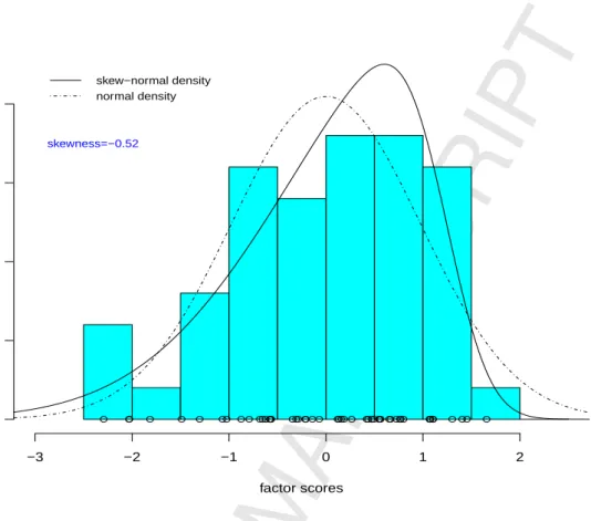
As a motivating example, we use the Versicolor subset of Fisher’s Iris data [20]. There are a total of 50 samples with each containing four-dimensional measurements in centimeters on the attributes of petal length, petal width, sepal length and sepal width. First, we employ a one-factor FA using the ML method for the data. Fig. 1 depicts the histogram of estimated factor scores in which the patterns are markedly skewed to the left with sample skewness equal to –0.52. Table 1 reports the ML re-sults obtained by fitting the FA and SNFA models with q= 1 to the Versicolor data. The proportion of the total sample variances explained by the factor is larger under SNFA (69.7%) than under FA (66.6%). The ML estimate of the skewness parameter
λ is −5.68 and its standard error is 0.29, supporting strongly non-normality of the underlying factor.
Since the maximized likelihood values of the two fitted models are obtained, we perform the likelihood ratio test (LRT) for testing the hypothesis H0 : λ= 0 (FA)
against H1 : λ6= 0 (SNFA). The resulting LRT statistic is 4.52 with p-value 0.034,
which is significant compared with aχ2
1distribution, giving the other indication that
the SNFA model is superior to the conventional FA. The χ21 distribution would be the limiting null distribution if regularity conditions hold [17]. Moreover, the sample skewness of the factor scores estimated by SNFA is –0.65, which exhibits a stronger left skew than does FA. In this regard, the “missed skewness” by the FA is then corrected to some extent by the SNFA.
We consider also the fitting of the MSNFA model to the full set of Fisher’s Iris data, which contains four geometric measurements of 50 samples from each of the three species of Iris (Setosa, Versicolor, and Virginica). For this illustration, the true number of clusters is taken to be unknown. Hence, the MSNFA model was applied to the data with g ranging from 1 to 4. The number of latent factors qis fixed at 1 to satisfy the restriction (p−q)2 ≥(p+q) as given by Eq. (8.5) of McLachlan and
Peel (2000). For comparison, we also implement the MSTFA and MCSTFA models via the alternating expectation conditional maximization (AECM) algorithms de-scribed by [59,60], respectively. When implementing the estimating procedure, the component dfs are restricted to be equal for stabilizing the convergence. A summary of the results are listed in Table 2.
To compare the clustering performance of these models, we report in Table 2 the associated ARI and CCR values for each model considered. It can be observed that BIC selects the correct number of clusters (g = 3) for the MSNFA model and it attains its highest CCR and ARI for g = 3 (CCR=0.980 and ARI=0.941). The MSTFA model also attains its highest values for g= 3, which are not as high as for the MSNFA model (CCR=0.973 and ARI=0.922). Also, BIC suggests g = 2 rather than g = 3 clusters for MSTFA. The use of the ICL criterion selects g = 2 clusters for both the MSNFA and MSTFA models. The performance of the MCSTFA model can be seen to be much poorer than that for the MSNFA and MCSTFA models. Cross-tabulation of the true and predicted class memberships (Table 3) shows that both models can perfectly separate Setosa and Virginica samples from the other two species. The MCSTFA approach does not perform relatively well for this dataset as not a large number of parameters are needed to characterize the structure of clusters.
6.2 The WDBC dataset
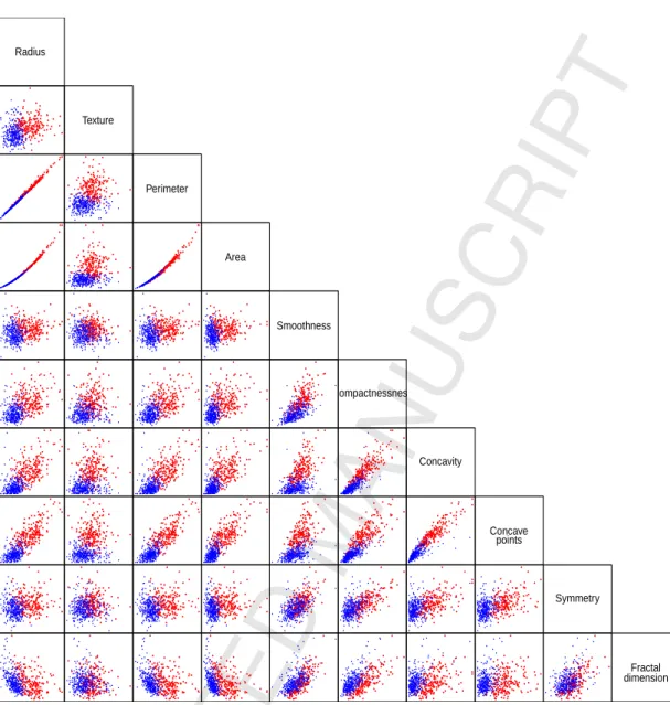
Breast cancer is a major cause of death for women. Early detection of breast cancer through classification can avoid unnecessary surgery. As another illustration, we applied our method to the Wisconsin Diagnostic Breast Cancer (WDBC) data, which are available from the UCI Machine Learning data repository [25]. These data consist of n= 569 instances with a total of 32 different attributes. The first two at-tributes correspond to the ID number and the diagnosis status, of which 357 have the diagnosis benign and 212 have the diagnose malignant. The rest p= 30 attributes are ten real-valued measurements (Radius, Texture, Perimeter, Area, Smoothness, Compactness, Concavity, Concave points, Symmetry and Fractal dimension) com-puted from a digitized mammography image of a fine needle aspirates (FNA) of breast tissue, together with their associated mean, standard error and the mean of the three largest (‘worst’) values, respectively. Fig. 2 displays the scatterplots of the
first 10 quantitative features. One can observe that many of these plots are appar-ently bimodal and appear to have rather non-elliptical patterns for both benign and malignant samples.
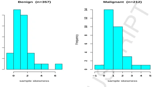
Fig. 3 shows the histograms of sample skewness of the corresponding 30 vari-ables in benign and malignant samples. It is readily seen that most of the varivari-ables exhibit highly positive skewness. There are indeed over half of the variables with skewness greater than one. This motivates us to advocate the use of MSNFA model to analyze this dataset.
Since there are two known classes, we implemented two-component MFA and MSNFA models with qranging from 1 to 10. To fit the models via the ML method, the ECM algorithm developed in Section 4.2 was employed under twenty different initializations for the parameters. The resulting ML solutions, including the maxi-mized log-likelihood values, the number of parameters together with the BIC and ICL values are listed in Table 4. To compare the classification accuracy, we also computed the ARI and CCR for each q. As can be seen, the best fitted model is MSNFA with q = 9, no matter which model selection criterion was used. In addi-tion, the resulting ARI (0.712) and CCR (0.923) under the fitted MSNFA (q = 9) are higher than all those under MFA models, although the MSNFA reaches its best ARI (0.762) and CCR (0.937) when q = 7. The result confirms that the MSNFA is more appropriate for this dataset, providing more accurate classification for this dataset, which exhibits a departure from normality. Finally, we did attempt to com-pare our MSNFA method with the MSTFA and MCSTFA models [63,64], but we encountered certain convergence problem when implementing the latter two models for this dataset.
6.3 Seeds data
Our third example concerns the seeds dataset analyzed by Charytanowicz and Niewczas [15]. Seven geometric features (area, perimeter, compactness, length of kernel, width of kernel, asymmetry coefficient, and length of kernel groove) were measured from theX-ray images of 210 wheat kernels. These grains belong to three different wheat varieties, namely Kama, Rosa, and Canadian. We consider the fitting of the MFA, MSNFA, MSTFA, and MCSTFA models to this dataset, withqvarying
from 1 to 3. Focusing first on the case where g is a priori known to be 3, it can be observed from Table 5 that the model with q= 3 is preferred by both the BIC and ICL for the MFA and MSTFA models. For the GHST factor models (see Table 6), the MSTFA model obtained its lowest BIC and ICL values when q = 3, whereas q= 2 is preferred by BIC and ICL for the MCSTFA model. However, their performances in clustering were relatively poor in terms of ARI and CCR.
We consider also the fitting of these factor models to the seeds data when g
is taken to be unknown. The MFA, MSNFA, MSTFA, and MCSTFA models were applied to the data with g ranging from 1 to 4. As above, the number of latent factors q varies from 1 to 3. On comparing their results reported in Tables 5 and 6, it can be observed that the model corresponding to g = 3 andq= 3 is preferred by both BIC and ICL for the MFA and MSNFA model, with the latter obtaining lower BIC and ICL values. For the MSTFA and MCSFTA models, a model with g = 2 would be chosen based on BIC and ICL. In this example, the highest ARI and CCR is given by the MSNFA model with q = 3 (ARI=0.7505 and CCR=0.9095), which coincides with the model selected by BIC and ICL. We note in Table 6 that the likelihood does not always increase with g and/or q for the MSTFA and MCSTFA models, indicating the convergence problems we encountered in the fitting of these two models.
6.4 A simulation study
We undertook a simulation study to examine the goodness of fit and clustering ability in simulated data by applying the proposed MSNFA model. To conduct experimental studies, we generated data sets inR10of sizeneach from a 3-component
MSNFA model with q= 2 factors. The presumed parameters are given as
w1= w2 =w3 = 1/3, µ1= 1110, µ2 = 2110, µ3 = 3110
Bi = Unif(10,2), Di = diag{Unif(10,1)}, λi =λ12, (i= 1,2,3),
where Unif(r, s) denotes a r×s matrix of random numbers drawn from a uniform distribution on the unit (0,1) interval and 1p is ap×1 vector of ones.
As pointed out by Wall et al. [72], the skewness of generated latent factors may become much smaller than the actual population values when the sample size n is
not large enough. In this study, we therefore consider somewhat large sample sizes (n = 600,1200, and 2400) to enhance the skewness effects. The specific values ofλ
are chosen as 0, 5, and 10. The higher the value of λ, the stronger the departure from the normality, while the zero-skewness λ= 0 corresponds to be normal factors. For comparison purposes, each simulated data set was fitted under the MFA and MSNFA scenarios along with the MSTFA model of Murray et al. [63] withg= 3 and
q = 2. The total number of free parameters in the three models are 119, 125 and 152, respectively. Compared with the formulation of MSNFA, the MSTFA model involves a much larger number of unknown parameters because its factor analytic representation applies to the error terms rather than the latent factors.
A total of 100 replications were run across each combination ofnandλ. The com-parison between the three models is made using BIC and ARI, which are commonly adopted to evaluate model fitting and classification performances, respectively. Ta-ble 7 lists the average BIC and ARI values and the corresponding standard devia-tions. To evaluate the objective use of the criteria, the frequencies preferred by BIC and ARI are also listed in the table. When λ = 0, it is not surprising that MFA is more likely to be selected. When focusing on the cases of non-zero skewness, the BIC scores provide a 53%–100% agreement with the specification of MSNFA, and the percentage of correctly choosing the true model increases with the sample size and the value of skewness parameter. In this study, the MSTFA model does not work well as it is strongly penalized due to over-fitting.
With regard to the MAP classification, the results indicate that when the la-tent factors approach normality (λ= 0), all three models produce comparable ARI values. When the latent factors are moderately and highly skewed (λ = 5,10), the MSNFA model yields slightly higher classification accuracies and is preferred more often than the other two models. Such a phenomenon becomes apparent as the sam-ple size increases. In summary, the MNSFA model can provide greater flexibility in model fitting and superiority for clustering in the presence of skew factors, at least for the setting of parameters used in this study.
7 Conclusion
We have proposed the MSNFA model by replacing the normal latent factors in the classical MFA model with the rMSN distributed factors for each component. This family of mixture factor analyzers has emerged as an attractive tool since it can account for groups in the data exhibiting patterns of asymmetry and multimodal-ity which are commonly seen in high-dimensional data. For estimating parameters, an analytically simple ECM algorithm is developed under a four-level hierarchical framework. Some computational strategies related to the specification of starting values, convergence assessment and provision of standard errors are provided. Two main identification problems regarding invariant likelihood caused by factor inde-terminacy and label switching are also discussed. We should mention that both of which do not affect the clustering results. Numerical results on model choice based on information-based criteria and apparent error rate for summarizing classification accuracy indicate the effectiveness and superiority of the proposed method when compared with the traditional MFA.
There are a number of possible extensions of the current work. While the pro-posed MSNFA has shown its flexibility in modeling asymmetric features among heterogeneous data, its robustness against outliers could still be unduly influenced by heavy-tailed observations. Mixtures of factor analyzers based on a more general family of distributions such as the skew t-distribution and its variants [6,32,38,66,67] would be of interest for future research. For identifying the optimal number of clus-ters, an effective method is to design a mixture component merging procedure using entropy as the criterion suggested by Baudry et al. [11]. Melnykov [55] further de-rived the asymptotic distribution of entropy and applied it to find good cluster partitions. Another worthwhile task is to develop workable Markov chain Monte Carlo algorithms for drawing inferences under a Bayesian paradigm. Although the proposed ECM procedure is quite easy to implement, its convergence can be slow in certain situations. Therefore, pursuing some modified algorithms such as [76,79] toward fast convergence deserves further investigation.
Acknowledgements
We gratefully acknowledge the Chief Editor, the Associate Editor and two anony-mous referees for their comments and suggestions, which have led to a much im-proved version of this article. This research was supported by MOST 103-2118-M-005-001-MY2 awarded by the Ministry of Science and Technology of Taiwan.
References
[1] K. Aas, I.H. Haff, The generalized hyperbolic skew Student’st-distribution. J. Financ.
Econom. 4 (2005) 275–309.
[2] R. Arellano-Valle, A. Azzalini, On the unification of families of skew-normal distributions. Scand. J. Statist. 33 (2006) 561–574.
[3] R. Arellano-Valle, M. Genton, On fundamental skew distributions. J. Multivariate Anal. 96 (2005) 93–116.
[4] A. Azzalini, The skew-normal distribution and related multivariate families. Scand. J. of Statist. 32 (2005) 159–188.
[5] A. Azzalini, A. Capitanio, Statistical applications of the multivariate skew normal distribution. J. R. Stat. Soc. Ser. B 61 (1999) 579–602.
[6] A. Azzalini, A. Capitanio, Distributions generated by perturbation of symmetry with emphasis on a multivariate skew t-distribution. J. R. Stat. Soc. Ser. B 65 (2003)
367–389.
[7] A. Azzalini, A. Dalla Valle, The multivariate skew-normal distribution. Biometrika 83 (1996) 715–726.
[8] J. Baek, G.J. McLachlan, Mixtures of common t-factor analyzers for clustering
high-dimensional microarray data. Bioinformatics 27 (2011) 1269–1276.
[9] J. Baek, G.J. McLachlan, L.K. Flack, Mixtures of factor analyzers with common factor loadings: applications to the clustering and visualization of high-dimensional data. IEEE Trans. Pattern Anal. Mach. Intell. 32 (2010) 1–13.
[10] O. Barndorff-Nielsen, N. Shephard, Non-Gaussian Ornstein-Uhlenbeck-based models and some of their uses in financial economics. J. R. Stat. Soc. Ser. B 63 (2001) 167–241.
[11] J.P. Baudry, A.E. Raftery, G. Celeux, K. Lo, R. Gottardo, Combining mixture components for clustering. J. Comput. Graph. Stat. 9 (2010) 332–353.
[12] C. Biernacki, G. Celeux, G. Govaert, Assessing a mixture model for clustering with the integrated completed likelihood. IEEE Trans. Pattern Anal. Mach. Intell. 22 (2000) 719–725.
[13] C. Biernacki, G. Celeux, G. Govaert, Choosing starting values for the EM algorithm for getting the highest likelihood in multivariate Gaussian mixture models. Comput. Stat. Data Anal. 41 (2003) 561–575.
[14] D. B¨ohning, Computer-Assisted Analysis of Mixtures and Applications: Meta-Analysis, Disease Mapping and Others. Chapman and Hall, New York, 1999.
[15] M. Charytanowicz, J. Niewczas, P. Kulczycki, P. Kowalski, S. Lukasik, S. Zak, A complete gradient clustering algorithm for features analysis of x-ray images, in: Information Technologies in Biomedicine, E. Pietka, J. Kawa (Eds), Springer, Berlin, 2010, pp. 15–24.
[16] A.P. Dempster, N.M. Laird, D.B. Rubin, Maximum likelihood from incomplete data via the EM algorithm (with discussion). J. Roy. Statist. Soc. B 39 (1977) 1–38. [17] M. Drton, Likelihood ratio tests and singularities, Ann. Statist. 37 (2009) 979–1012. [18] B. Efron, D.V. Hinkley, Assessing the accuracy of the maximum likelihood estimator:
observed versus expected Fisher information. Biometrika 65 (1978) 457–482.
[19] B.S. Everitt, D.J Hand, Finite Mixture Distributions. Chapman & Hall, London, 1981. [20] R. Fisher, The use of multiple measurements in taxonomic problems. Ann. Eugenics
7 (1936) 179–188.
[21] E. Fokou´e, D.M. Titterington, Mixtures of factor analyzers. Bayesian estimation and inference by stochastic simulation. Mach. Learning 50 (2003) 73–94.
[22] C. Fraley, Algorithms for model-based Gaussian hierarchical clustering. SIAM J. Sci. Comput. 20 (1998) 270–281.
[23] C. Fraley, A.E. Raftery, T.B. Murphy, L. Scrucca, MCLUST Version 4 for R: Normal Mixture Modeling and Model-Based Clustering, Technical Report 597, University of Washington, Department of Statistics, Seattle, WA. (2012)
[24] B.C. Franczak, P.D. McNicholas, R.P. Browne, P.M. Murray, Parsimonious shifted asymmetric Laplace mixtures. Preprint arXiv:1311.0317v1. (2013)
[25] A. Frank, A. Asuncion, UCI Machine Learning Repository. Irvine, CA: University of California, School of Information and Computer Science (2010). http://archive.ics.uci.edu/ml.
[26] S. Fr¨uhwirth-Schnatter, Finite Mixture and Markov Switching Models, Springer, New York, 2006.
[27] Z. Ghahramani, M. Beal, Variational inference for Bayesian mixture of factor analysers. In: Solla S, Leen T, Muller K-R (eds) Adv. Neur. Info. Proc. Sys. 12. MIT Press, Cambridge (2000) 449–455.
[28] Z. Ghahramani, G.E. Hinton, The EM algorithm for mixtures of factor analyzers. Technical report no. CRG-TR-96-1, University of Toronto (1997)
[29] L. Hubert, P. Arabie, Comparing partitions. J. Classif. 2 (1985) 193–218.
[30] M. Jamshidian, An EM algorithm for ML factor analysis with missing data. In Berkane, M. (Ed.) Latent Variable Modeling and Applications to Causality (1997) 247–258. Springer Verlag, New York.
[31] D. Karlis, E. Xekalaki, Choosing initial values for the EM algorithm for finite mixtures. Comput. Stat. Data Anal. 41 (2003) 577–590.
[32] V.H. Lachos, P. Ghosh, R.B. Arellano-Valle, Likelihood based inference for skew-normal/independent linear mixed model. Stat. Sin. 20 (2010) 303–322.
[33] S. Lee, G.J. McLachlan, On mixtures of skew normal and skew t-distributions. Adv.
Data Anal. Classif. 7, (2013a) 241–266.
[34] S. Lee, G.J. McLachlan, EMMIX-uskew: an R package for fitting mixtures of multivariate skew t-distributions via the EM algorithm. J. Statist. Software 55, No.
12. (2013b)
[35] S. Lee, G.J. McLachlan, Finite mixtures of multivariate skew t-distributions: some
recent and new results Statist. Comput. 24 (2014) 181–202.
[36] Y.W. Lee, S.H. Poon, Systemic and systematic factors for loan portfolio loss distribution. Econometrics and Applied Economics Workshops (2011). School of Social Science, University of Manchester, pp. 1–61.
[37] T.I. Lin, Maximum likelihood estimation for multivariate skew normal mixture models. J. Multivariate Anal. 100 (2009) 257–265.
[38] T.I. Lin, H.J. Ho, C.R. Lee, Flexible mixture modelling using the multivariate
[39] T.I. Lin, J.C. Lee, S.Y. Yen, Finite mixture modelling using the skew normal distribution, Stat. Sin. 17 (2007) 909–927.
[40] B.G. Lindsay, Mixture Models: Theory, Geometry, and Applications. NSF-CBMS Regional Conference Series in probability and Statistics, Volume 5, Institute of Mathematical Statistics, Hayward, CA, 1995.
[41] C.H. Liu, Efficient ML estimation of the multivariate normal distribution from incomplete data. J. Multivariate Anal. 69 (1999) 206–217.
[42] C.H. Liu, D.B. Rubin, Y.N. Wu, Parameter expansion to accelerate EM: the PX-EM algorithm. Biometrika 85 (1998) 755-770.
[43] H.F. Lopes, M. West, Bayesian model assessment in factor analysis. Stat. Sin. 4 (2004) 41–67.
[44] T.A. Louis, Finding the observed information when using the EM algorithm. J. R. Stat. Soc. Ser. B 44 (1982) 226–232.
[45] R. Maitra, Initializing partition-optimization algorithms. IEEE ACM T. Comput. Bi. 6 (2009) 144–157.
[46] R. Maitra, V. Melnykov, Simulating data to study performance of finite mixture modeling and clustering algorithms. J. Comput. Graph. Stat. 19 (2010) 354–376. [47] G.J. McLachlan, K.E. Basford, Mixture Models: Inference and Application to
Clustering, Marcel Dekker, New York, 1988.
[48] G.J. McLachlan, R.W. Bean, L.B.T. Jones, Extension of the mixture of factor analyzers model to incorporate the multivariate t-distribution. Comput. Stat. Data
Anal. 51 (2007) 5327–5338.
[49] G.J. McLachlan, R.W. Bean, D. Peel, A mixture model-based approach to the clustering of microarray expression data. Bioinformatics 18 (2002) 413–422.
[50] G.J. McLachlan, T. Krishnan, The EM Algorithm and Extensions, 2nd edn. Wiley, New York. 2008.
[51] G.J. McLachlan, D. Peel, Finite Mixture Models. Wiely, New York, 2000.
[52] G.J. McLachlan, D. Peel, Mixtures of factor analyzers. In Proceedings of the Seventeenth International Conference on Machine Learning. San Francisco: Morgan Kaufmann, pp. 599–606 (2000)
[53] G.J. McLachlan, D. Peel, R.W. Bean, Modelling high-dimensional data by mixtures of factor analyzers. Comput. Stat. Data Anal. 41 (2003) 379–388.
[54] P.D. McNicholas, T.B. Murphy, Parsimonious Gaussian mixture models. Statist. Comput. 18 (2008) 285–296.
[55] V. Melnykov, On the distribution of posterior probabilities in finite mixture models with application in clustering. J. Multivariate Anal. 122 (2013) 175–189.
[56] V. Melnykov, W.C. Chen, R. Maitra MixSim: an R package for simulating data to study performance of clustering algorithms. J. Stat. Softw. 51 (2012) 1–25.
[57] V. Melnykov, I. Melnykov, Initializing the EM algorithm in Gaussian mixture models with an unknown number of components. Comput. Stat. Data Anal. 56 (2012) 1381– 1395.
[58] X.L. Meng, D.B. Rubin, Using EM to obtain asymptotic variance-covariance matrices: The SEM algorithm. J. Amer. Statist. Assoc. 86 (1991) 899–909.
[59] X.L. Meng, D.B. Rubin, Maximum likelihood estimation via the ECM algorithm: a general framework. Biometrika 80 (1993) 267–278.
[60] K. Mengersen, C. Robert, D.M. Titterington, Mixtures: Estimation and Applications, John Wiley & Sons, Chichester, UK, 2011.
[61] A. Montanari, C. Viroli, A skew-normal factor model for the analysis of student satisfaction towards university courses. J. App. Statist. 37 (2010) 473–487.
[62] P. Murray, R. Browne, P.D. McNicholas, Mixtures of ‘unrestricted’ skew-t factor
analyzers. Preprint arXiv: 1310.6224v1. (2013)
[63] P.M. Murray, R. Browne, P.D. McNicholas, Mixtures of skew-t factor analyzers.
Comput. Stat. Data Anal. 77 (2014a) 326–335.
[64] P.M. Murray, P.D. McNicholas, R. Browne, Mixtures of common skew-t factor
analyzers. Stat 3 (2014b) 68–82.
[65] A. O’Hagan, T. Murphy, I. Gormley, Computational aspects of fitting mixture models via the expectation-maximization algorithm. Comput. Stat. Data Anal. 56 (2012) 3843–3864.
[66] S. Pyne, X. Hu, K. Wang, E. Rossin, T.I. Lin, L.M. Maier, C. Baecher-Allan, G.J. McLachlan, P. Tamayo, D.A. Hafler, P.L. De Jager, J.P. Mesirov, Automated high-dimensional flow cytometric data analysis. Proc. Natl. Acad. Sci (PNAS) USA, 106 (2009) 8519–8524.
[67] S.K. Sahu, D.K. Dey, M.D. Branco, A new class of multivariate skew distributions with application to Bayesian regression models. Can. J. Statist. 31 (2003) 129-150.
[68] G. Schwarz, Estimating the dimension of a model. Ann. Statist. 6 (1978) 461-464. [69] D.M., Titterington, A.F.M. Smith, U.E. Markov, Statistical Analysis of Finite Mixture
Distributions. Wiely, New York, 1985.
[70] C. Tortora, P.D. McNicholas, R. Browne, A mixture of generalized hyperbolic factor analyzers. arXiv: 1311.6530v1. (2013)
[71] A. Utsugi, T. Kumagai, Bayesian analysis of mixtures of factor analyzers. Neural Comp. 13 (2001) 993–1002.
[72] M.M. Wall, J. Guo, Y. Amemiya, Mixture factor analysis for approximating a non-normally distributed continuous latent factor with continuous and dichotomous observed variables. Multivar. Behav. Res. 47 (2012) 276–313.
[73] K. Wang, EMMIX-skew (R package version 1.0-12): EM algorithm for mixture of multivariate skew Normal/tdistributions (2009).
[74] W.L. Wang, Mixtures of common factor analyzers for high-dimensional data with missing information. J. Multivariate Anal. 117 (2013) 120–133.
[75] W.L. Wang, Mixtures of common t-factor analyzers for modeling high-dimensional
data with missing values. Comput. Stat. Data Anal. 83 (2015) 223–235.
[76] W.L. Wang, T.I. Lin, An efficient ECM algorithm for maximum likelihood estimation in mixtures oft-factor analyzers. Comput. Statist. 8 (2013) 751–769.
[77] J.H. Ward, Hierarchical grouping to optimize an objective function. J. Amer. Statist. Assoc. 58 (1963) 236–244.
[78] C.F.J. Wu, On the convergence properties of the EM algorithm. Ann. Stat. 11 (1983) 95–103.
[79] J.H. Zhao, P.L.H. Yu, Fast ML estimation for the mixture of factor analyzers via an ECM algorithm. IEEE. Trans. Neural Net. 19 (2008) 1956–1961.
Table 1
ML results for the Versicolor subset of the Iris data. Values within parentheses are the corresponding standard errors of ML estimates.
Variable MFA (g =q= 1) MSNFA (g= q= 1)
µ B d µ B d Sepal Length 5.936 0.395 0.105 5.942 0.403 0.105 (0.072) (0.063) (0.025) (0.090) (0.069) (0.029) Sepal Width 2.770 0.198 0.057 2.773 0.201 0.058 (0.044) (0.041) (0.012) (0.054) (0.053) (0.013) Petal Length 4.260 0.442 0.021 4.267 0.454 0.019 (0.066) (0.052) (0.015) (0.090) (0.097) (0.005) Petal Width 1.326 0.162 0.012 1.329 0.163 0.013 (0.028) (0.023) (0.003) (0.038) (0.027) (0.003) Proportion of 0.666 0.697 variance explained m 12 13 ℓmax –16.488 –14.229 LRT (p-value) 4.517 ( 0.034)
Table 2
Comparison of the fitted MSNFA, MSTFA and MCSTFA models on the Iris data. Model g ℓmax m BIC ICL ARI CCR
1 -419.3 13 903.8 903.8 0.000 0.333 MSNFA 2 -231.6 27 598.4 598.4 0.568 0.667 3 -192.8 41 591.2 600.6 0.941 0.980 4 -184.6 55 644.6 672.8 0.757 0.820 1 -387.4 17 860.0 860.0 0.000 0.333 MSTFAa 2 -214.4 34 599.2 599.2 0.568 0.667 3 -176.8 51 609.2 617.6 0.922 0.973 4 -170.7 68 680.8 692.6 0.727 0.807 1 -700.3 14 1470.8 1470.8 0.000 0.333 MCSTFAb 2 -686.4 21 1478.0 1583.8 0.185 0.553 3 -680.5 28 1501.2 1624.8 0.140 0.460 4 -676.1 35 1527.6 1698.2 0.238 0.440
MSTFAaand MCSTFAbindicate the mixture of skew-tfactor analyzers [63] and the mixture of common skew-tfactor analyzers [64],
respectively, based on the generalized hyperbolic skew-tdistribution.
Table 3
Cross-tabulations of true and predicted class memberships for the selected MSNFA and MSTFA models on the Iris data.
MSNFA MSTFA
1 2 3 1 2 3
Setosa 50 0 0 50 0 0
Versicolor 0 47 3 0 46 4
Table 4
Comparison of MFA and MSNFA fitting results and implied clustering versus the true membership of WDBC data.
Model q ℓmax m BIC ICL ARI CCR
1 9624.8 181 -18101.4 -18083.8 0.520 0.861 2 12362.7 239 -23209.2 -23193.2 0.396 0.817 3 13962.5 295 -26053.6 -26043.4 0.359 0.803 4 15616.8 349 -29019.6 -29013.6 0.658 0.907 MFA 5 15726.5 401 -28909.2 -28897.4 0.595 0.888 6 16691.4 451 -30521.6 -30513.4 0.630 0.898 7 17017.2 499 -30868.8 -30862.0 0.670 0.910 8 17248.6 545 -31039.8 -31030.6 0.595 0.888 9 18467.3 589 -33198.0 -33190.8 0.700 0.919 10 17692.3 631 -31381.6 -31370.0 0.624 0.896 1 9632.8 183 -18104.8 -18086.2 0.515 0.859 2 12441.3 243 -23341.0 -23325.2 0.373 0.808 3 14117.8 301 -26326.2 -26317.2 0.397 0.817 4 15700.5 357 -29136.2 -29127.6 0.658 0.907 MSNFA 5 15830.1 411 -29053.0 -29042.6 0.618 0.895 6 16933.3 463 -30929.4 -30918.6 0.718 0.924 7 17486.8 513 -31719.2 -31712.0 0.762 0.937 8 17572.5 561 -31586.0 -31579.0 0.681 0.914 9 18598.8 607 -33347.0 -33340.4 0.712 0.923 10 18000.9 651 -31872.0 -31862.8 0.700 0.919
Table 5
Comparison of the fitted MFA and MSNFA models on the seeds data.
Model g q ℓmax m BIC ICL ARI CCR
1 1 75.74 21 -39.20 -156.80 0.0000 0.3333 1 2 105.05 27 -65.73 -262.93 0.0000 0.3333 1 3 680.75 32 -1190.39 -4761.58 0.0000 0.3333 2 1 265.34 43 -300.75 -1176.00 0.4191 0.6571 2 2 274.18 55 -254.28 -998.27 0.4388 0.6571 MFA 2 3 1026.80 65 -1706.03 -6814.15 0.4685 0.6667 3 1 419.77 65 -491.98 -1945.11 0.4261 0.7667 3 2 385.98 83 -328.14 -1286.14 0.4189 0.7619 3 3 1201.36 98 -1878.71 -7503.86 0.6875 0.8810 4 1 396.86 87 -328.52 -1294.94 0.4891 0.7429 4 2 540.57 111 -487.61 -1925.27 0.4430 0.6476 4 3 1255.09 131 -1809.72 -7218.28 0.6043 0.7381 1 1 80.68 22 -43.73 -174.92 0.0000 0.3333 1 2 112.00 29 -68.94 -275.77 0.0000 0.3333 1 3 685.99 35 -1184.82 -4739.29 0.0000 0.3333 2 1 303.42 45 -366.21 -1416.58 0.2868 0.6000 2 2 278.44 59 -241.39 -937.19 0.4257 0.6524 MSNFA 2 3 1034.95 71 -1690.26 -6751.42 0.4720 0.6667 3 1 505.52 68 -647.44 -2570.41 0.1253 0.5238 3 2 476.50 89 -477.10 -1878.65 0.2363 0.6333 3 3 1207.38 107 -1842.61 -7357.09 0.7505 0.9095 4 1 368.88 91 -251.18 -961.32 0.4517 0.7238 4 2 816.30 119 -996.29 -3951.51 0.2632 0.5143 4 3 1280.77 143 -1796.90 -7167.82 0.5971 0.7333
Table 6
Results of the fitted MSTFA and MCSTFA models on the seeds data.
Model g q ℓmax m BIC ICL ARI CCR
1 1 535.65 29 -916.24 -3664.95 0.0000 0.3333 1 2 565.63 35 -944.12 -3776.47 0.0000 0.3333 1 3 673.56 40 -1133.25 -4532.98 0.0000 0.3333 2 1 809.71 59 -1303.94 -5193.91 0.4268 0.6524 2 2 733.04 71 -1086.44 -4331.91 0.4372 0.6286 MSTFA 2 3 1047.10 81 -1661.07 -6624.61 0.4685 0.6667 3 1 469.99 89 -464.09 -1808.96 0.5216 0.8238 3 2 829.82 107 -1087.50 -4314.84 0.4664 0.7476 3 3 1071.08 122 -1489.81 -5940.30 0.3975 0.6333 4 1 542.17 119 -448.04 -1656.63 0.3651 0.6333 4 2 754.36 143 -744.08 -2939.44 0.5776 0.7762 1 1 -609.55 23 1342.08 5368.33 0.0000 0.3333 1 2 113.49 30 -66.58 -266.30 0.0000 0.3333 1 3 -301.87 36 796.23 3184.93 0.0000 0.3333 2 1 -607.92 34 1397.64 5594.50 0.0000 0.3381 MCSTFA 2 2 -751.58 44 1738.43 6953.74 2.0096 0.3333 2 3 540.83 54 -792.92 -3167.05 0.0002 0.3429 3 1 -978.40 45 2197.43 9006.83 0.2199 0.5571 3 2 175.25 58 -40.38 -27.31 0.5103 0.8048 3 3 -893.33 72 2171.64 8821.90 0.1243 0.5000
Table 7
Simulation results based on 100 replications.
λ= 0 λ= 5 λ= 10
MFA MSNFA MSTFAa MFA MSNFA MSTFAa MFA MSNFA MSTFAa
n= 600 Mean –7746.56 –7762.45 –7821.87 –7746.58 –7743.88 –7816.90 –7871.05 –7865.28 –7939.25 BIC Std 341.70 342.46 342.47 335.16 362.39 337.12 358.66 362.49 359.65 Freq 98 2 0 47 53 0 40 60 0 Mean 0.717 0.716 0.706 0.719 0.732 0.714 0.680 0.697 0.672 ARI Std 0.092 0.092 0.099 0.088 0.085 0.092 0.097 0.095 0.104 Freq 37 34 29 15 65 20 15 69 16 n= 1200 Mean –15319.82 –15338.41 –15409.79 –15246.60 –15228.07 –15318.34 –15330.90 –15307.24 –15399.61 BIC Std 785.44 785.75 785.97 804.30 807.57 805.04 784.52 792.12 787.92 Freq 98 2 0 24 76 0 15 85 0 Mean 0.715 0.715 0.708 0.728 0.742 0.729 0.713 0.730 0.713 ARI Std 0.080 0.080 0.082 0.089 0.084 0.089 0.094 0.088 0.094 Freq 25 44 31 11 68 21 10 75 15 n= 2400 Mean –30409.19 –30428.81 –30513.46 –30178.59 –30129.58 –30245.06 –30423.53 –30350.51 –30488.06 BIC Std 1407.30 1405.85 1405.87 1390.61 1400.14 1393.94 1422.68 1433.58 1426.50 Freq 98 2 0 1 99 0 0 100 0 Mean 0.727 0.727 0.723 0.727 0.739 0.730 0.721 0.739 0.726 ARI Std 0.075 0.075 0.077 0.071 0.067 0.069 0.087 0.082 0.085 Freq 35 37 28 4 76 20 1 84 15
factor scores Density −3 −2 −1 0 1 2 0.0 0.1 0.2 0.3 0.4 skew−normal density normal density skewness=−0.52
Fig. 1. Histogram of the factor scores obtained by fitting FA (q = 1) together with the
Radius Texture Perimeter Area Smoothness Compactnessness Concavity Concave points Symmetry Fractal dimension
Fig. 2. Pairwise scatterplots of the first 10 quantitative features. The blue dot represents benign samples, and the red cross represents malignant samples.
Benign (n=357) sample skewness Frequency 0 2 4 6 0 2 4 6 8 10 Malignant (n=212) sample skewness Frequency −1 0 1 2 3 4 5 0 2 4 6 8 10 12 14
Fig. 3. Histograms of sample skewness of the corresponding 30 quantitative in benign and malignant samples.