Pig Program Optimization and Creative Design

Performance Modeling and Optimization of Deadline-Driven Pig

Programs

ZHUOYAO ZHANG, University of Pennsylvania

LUDMILA CHERKASOVA, Hewlett-Packard Labs

ABHISHEK VERMA, University of Illinois at Urbana-Champaign

BOON THAU LOO, University of Pennsylvania

Many applications associated with live business intelligence are written as complex data analysis programs defined by directed acyclic graphs of MapReduce jobs, e.g. using Pig, Hive, or Scope frameworks. An in-creasing number of these applications have additional requirements for completion time guarantees. In this paper, we consider the popular Pig framework that provides a high-level SQL-like abstraction on top of MapReduce engine for processing large data sets. There is a lack of performance models and analysis tools for automated performance management of such MapReduce jobs. We offer a performance modeling envi-ronment for Pig programs that automatically profiles jobs from the past runs and aims to solve the following inter-related problems: (i) estimating the completion time of a Pig program as a function of allocated re-sources; (ii) estimating the amount of resources (a number of map and reduce slots) required for completing a Pig program with a given (soft) deadline. First, we design abasicperformance model that accurately pre-dicts completion time and required resource allocation for a Pig program that is defined as a sequence of MapReduce jobs: predicted completion times are within 10% of the measured ones. Second, we optimize a Pig program execution by enforcing theoptimal scheduleof its concurrent jobs. For DAGs with concurrent jobs, this optimization helps reducing the program completion time: 10%-27% in our experiments. Moreover, it eliminates possible non-determinism of concurrent jobs’ execution in the Pig program, and therefore, en-ables a more accurate performance model for Pig programs. Third, based on these optimizations, we propose arefinedperformance model for Pig programs with concurrent jobs. The proposed approach leads to signifi-cant resource savings (20%-60% in our experiments) compared with the original, unoptimized solution. We validate our solution using a 66-node Hadoop cluster and a diverse set of workloads: PigMix benchmark, TPC-H queries, and customized queries mining a collection of HP Labs’ web proxy logs.

Categories and Subject Descriptors: C.4 [Computer System Organization]: Performance of Systems; C.2.6 [Software]: Programming Environments

General Terms: Algorithms, Design, Performance, Measurement, Management Additional Key Words and Phrases: Hadoop, Pig, Resource Allocation, Scheduling 1. INTRODUCTION

The amount of useful enterprise data produced and collected daily is exploding. This is partly due to a new era of automated data generation and massive event logging of automated and digitized business processes; new style customer interactions that are done entirely via web; a set of novel applications used for advanced data analytics in call centers and for information management associated with data retention, gov-ernment compliance rules, e-discovery and litigation issues that require to store and This work was originated and largely completed during Z. Zhang’s and A. Verma’s internship at HP Labs. B. T. Loo and Z. Zhang are supported in part by NSF grants (CNS-1117185, CNS-0845552 , IIS- 0812270). A. Verma is supported in part by NSF grant CCF-0964471.

Permission to make digital or hard copies of part or all of this work for personal or classroom use is granted without fee provided that copies are not made or distributed for profit or commercial advantage and that copies show this notice on the first page or initial screen of a display along with the full citation. Copyrights for components of this work owned by others than ACM must be honored. Abstracting with credit is per-mitted. To copy otherwise, to republish, to post on servers, to redistribute to lists, or to use any component of this work in other works requires prior specific permission and/or a fee. Permissions may be requested from Publications Dept., ACM, Inc., 2 Penn Plaza, Suite 701, New York, NY 10121-0701 USA, fax+1 (212) 869-0481, or [email protected].

c

YYYY ACM 1556-4665/YYYY/01-ARTA $15.00

process large amount of historical data. Many companies are following the new wave of using MapReduce [Dean and Ghemawat 2008] and its open-source implementation Hadoop to quickly process large quantities of new data to drive their core business. MapReduce offers a scalable and fault-tolerant framework for processing large data sets. It is based on two main primitives:mapandreducefunctions that, in essence, per-form agroup-by-aggregationin parallel over the cluster. While initially this simplicity looks appealing to programmers, at the same time, it causes a set of limitations. One-input data set and simple two-stage dataflow processing schema imposed by MapRe-duce model is a low level and rigid. For analytics tasks that are based on a different dataflow, e.g.,joinsorunions, a special work around needs to be designed. This leads to programs with obscure semantics which are difficult to reuse. To enable programmers to specify more complex queries in an easier way, several projects, such as Pig [Gates et al. 2009], Hive [Thusoo et al. 2009], Scope [Chaiken et al. 2008], and Dryad [Isard et al. 2007], provide high-level SQL-like abstractions on top of MapReduce engines. These frameworks enable complex analytics tasks (expressed as high-level declarative abstractions) to be compiled intodirected acyclic graphs(DAGs) of MapReduce jobs.

Another technological trend is the shift towards using MapReduce and the above frameworks in support of latency-sensitive applications, e.g., personalized advertis-ing, sentiment analysis, spam and fraud detection, real-time event log analysis, etc. These MapReduce applications typically require completion time guarantees and are deadline-driven. Often, they are a part of an elaborate business pipeline, and they have to produce results by a certain time deadline, i.e., to achieve certain performance goals and service level objectives (SLOs). While there have been some research ef-forts [Verma et al. 2011a; Wolf et al. 2010; Polo et al. 2010] towards developing perfor-mance models for MapReduce jobs, these techniques do not apply to complex queries consisting of MapReduce DAGs. To address this limitation, our paper studies the pop-ular Pig framework [Gates et al. 2009], and aims to design a performance modeling environment for Pig programs to offer solutions for the following problems:

• Given a Pig program, estimate its completion time as a function of allocated re-sources (i.e., allocated map and reduce slots);

• Given a Pig program with a completion time goal, estimate the amount of resources (a number of map and reduce slots) required for completing the Pig program with a given (soft) deadline.

We focus on Pig, since it is quickly becoming a popular and widely-adopted system for expressing a broad variety of data analysis tasks. With Pig, the data analysts can specify complex analytics tasks without directly writing Map and Reduce func-tions. In June 2009, more than 40% of Hadoop production jobs at Yahoo! were Pig programs [Gates et al. 2009]. While our paper is based on the Pig experience, we be-lieve that the proposed models and optimizations are general and can be applied for performance modeling and resource allocations of complex analytics tasks that are expressed as an ensemble (DAG) of MapReduce jobs.

In addressing the above two problems, the paper makes the following contributions: Basic performance model. We propose a simple and intuitive basic performance model that accurately predicts a completion time and required resource allocation for a Pig program that is defined as asequenceof MapReduce jobs. Our model uses MapRe-duce job profiles extracted automatically from previous runs of the Pig program. The profiles reflect critical performance characteristics of the underlying application dur-ing its execution, and are built without requirdur-ing any modifications or instrumentation of either the application or the underlying Hadoop/Pig execution engine. All this infor-mation can be automatically obtained from the counters at the job master during the

job’s execution or alternatively parsed from the job logs. Our evaluation of the basic model with PigMix benchmark [Apache 2010] on a 66-node Hadoop cluster shows that the predicted completion times are within 10% of the measured ones, and the proposed model results in effective resource allocation decisions for sequential Pig programs. Pig scheduling optimizations. When a Pig program is defined by a DAG with con-current jobs, the proposedbasicmodel is pessimistic, i.e., the predicted completion time is higher than the measured one. The reason is that unlike the execution of sequential jobs where the next job can only start after the previous one is completed, for concur-rent jobs, once the previous job completes its map phase and begins its reduce phase, the next job can start its map phase execution with the released map resources in a pipelined fashion. The performance model should take this “overlap” in executions of concurrent jobs into account. Moreover, the random order of concurrent jobs’ execution by Hadoop scheduler may lead to inefficient resource usage and increased processing time. Using this observation, we first, optimize a Pig program execution by enforcing the optimal scheduleof its concurrent jobs. We evaluate optimized Pig programs and the related performance improvements using TPC-H queries and a set of customized queries mining a collection of HP Labs’ web proxy logs (both sets are presented by the DAGs with concurrent jobs). Our results show 10%-27% decrease in Pig program completion times.

Refined performance model. The proposed Pig optimization has another useful outcome: it eliminates existing non-determinism in Pig program execution of concur-rent jobs, and therefore, it enables better performance predictions. We develop an accu-raterefinedperformance model for completion time estimates and resource allocations of optimized Pig programs. We validate the accuracy of therefinedmodel using a com-bination of TPC-H and web proxy log analysis queries. Moreover, we show that for Pig programs with concurrent jobs, this approach leads to significant resource savings (20%-60% in our experiments) compared with the original, non-optimized solution.

This paper is organized as follows. Section 2 provides a background on MapReduce and Pig frameworks. Section 3 introduces abasicperformance model for Pig programs with completion time goals. This model is evaluated in Section 4. Section 5 proposes an optimized scheduling of concurrent jobs in Pig program and introduces a refined performance model. The accuracy of the new model is evaluated in Section 6. Section 7 discusses the challenges in Pig programs modeling with different size input datasets. Section 8 describes the related work. Section 9 presents a summary and future direc-tions.

2. BACKGROUND

This section provides a basic background on the MapReduce framework [Dean and Ghemawat 2008] and its extension, the Pig system, that offers a higher-level abstrac-tion for expressing more complex analytic tasks using SQL-style constructs.

2.1. MapReduce Jobs

In the MapReduce model, computation is expressed as two functions: map and reduce. The map function takes an input pair and produces a list of intermediate key/value pairs. The reduce function then merges or aggregates all the values associated with the same key.

MapReduce jobs are automatically parallelized, distributed, and executed on a large cluster of commodity machines. The map and reduce stages are partitioned into map and reduce tasks respectively. Each map task processes a logical split of input data that generally resides on a distributed file system. The map task reads the data, applies the user-defined map function on each record, and buffers the resulting output. This data

is sorted and partitioned for different reduce tasks, and written to the local disk of the machine executing the map task. The reduce stage consists of three phases: shuffle, sort and reduce phase. In the shuffle phase, the reduce tasks fetch the intermediate data files from the already completed map tasks, thus following the “pull” model. In the sort phase, the intermediate files from all the map tasks are sorted. An external merge sort is used in case the intermediate data does not fit in memory as follows: the intermediate data is shuffled, merged in memory, and written to disk. After all the intermediate data is shuffled, a final pass is made to merge all these sorted files, hence interleaving the shuffle and sort phases. Finally, in the reduce phase, the sorted intermediate data is passed to the user-defined reduce function. The output from the reduce function is generally written back to the distributed file system.

Job scheduling in Hadoop is performed by a master node, which manages a number of worker nodes in the cluster. Each worker has a fixed number ofmap slotsandreduce slots, which can run map and reduce tasks respectively. The number of map and reduce slots is statically configured (typically, one or two per core or disk). The slaves periodi-cally send heartbeats to the master to report the number of free slots and the progress of tasks that they are currently running. Based on the availability of free slots and the scheduling policy, the master assigns map and reduce tasks to slots in the cluster. 2.2. Pig Programs

The current Pig system consists of the following main components:

• The language, called Pig Latin, that combines high-level declarative style of SQL and the low-level procedural programming of MapReduce. A Pig program is similar to specifying a query execution plan: it represent a sequence of steps, where each one carries a single data transformation using a high-level data manipulation con-structs, like filter, group, join, etc. In this way, the Pig program encodes a set of explicit dataflows.

• Theexecution environment to run Pig programs. The Pig system takes a Pig Latin program as input, compiles it into a DAG of MapReduce jobs, and coordinates their execution on a given Hadoop cluster. Pig relies on underlying Hadoop execution en-gine for scalability and fault-tolerance properties.

The following specification shows a simple example of a Pig program. It describes a task that operates over a tableURLsthat stores data with the three attributes: (url,

category, pagerank). This program identifies for eachcategorytheurlwith the

high-estpagerankin thatcategory.

URLs =load’dataset’ as (url, category, pagerank); groups =groupURLs by category;

result =foreachgroups generate group, max(URLs.pagerank); storeresult into ’myOutput’

The example Pig program is compiled into a single MapReduce job. Typically, Pig programs are more complex, and can be compiled into an execution plan consisting of several stages of MapReduce jobs, some of which can run concurrently. The structure of the execution plan can be represented by a DAG of MapReduce jobs that could con-tain both concurrent and sequential branches. Figure 1 shows a possible DAG of five MapReduce jobs {j1, j2, j3, j4, j5}, where each node represents a MapReduce job, and the edges between the nodes represent thedata dependenciesbetween jobs.

To execute the plan, the Pig engine will first submit all theready jobs (i.e., the jobs that do not have data dependency on the other jobs) to Hadoop. After Hadoop has processed these jobs, the Pig system will delete those jobs and the corresponding edges from the processing DAG, and will identify and submit the next set of ready jobs. This

J1

J2

J3

J4

J5 J6

Fig. 1. Example of a Pig program’ execution plan represented as a DAG of MapReduce jobs. process continues until all the jobs are completed. In this way, the Pig engine partitions the DAG into multiple stages, each containing one or more independent MapReduce jobs that can be executed concurrently.

For example, the DAG shown in Figure 1 will be partitioned into the following four stages for processing:

— first stage:{j1, j2}; — second stage:{j3, j4}; — third stage:{j5}; — fourth stage:{j6}.

In Section 4, we will show some examples based on TPC-H and web log analysis queries that are representative of such MapReduce DAGs. Note that for stages with concurrent jobs, there is no specifically defined ordering in which the jobs are going to be executed by Hadoop, For example, for a first stage in our example it could bej1 followed byj2, orj2 followed byj1. This random ordering leads to a non-determinism in the Pig program execution that might have significant performance implications as we will see in Section 5.

3. BASIC PERFORMANCE MODEL

In this section, we introduce abasicperformance model for predicting completion time and resource allocation of a Pig program with performance goals. This model is simple, intuitive, and effective for estimating the completion times of sequential Pig programs. 3.1. Performance Model for Single MapReduce

As a building block for modeling Pig programs defined as DAGs of MapReduce jobs, we apply a slightly modified approach introduced in [Verma et al. 2011a] for perfor-mance modeling of a single MapReduce job. The proposed MapReduce perforperfor-mance model [Verma et al. 2011a] evaluates the lower and upper bounds on the job comple-tion time. It is based on a general model for computing performance bounds on the completion time of a given set ofntasks that are processed bykservers, (e.g.,nmap tasks are processed by kmap slots in MapReduce environment). LetT1, T2, . . . , Tn be the duration ofntasks in a given set. Letkbe the number of slots that can each exe-cute one task at a time. The assignment of tasks to slots is done using an online,greedy algorithm: assign each task to the slot which finished its running task the earliest. Let avgandmaxbe theaverageandmaximumduration of thentasks respectively. Then the completion time of a greedy task assignment is proven to be at least:

Tlow =avg· n k and at most

Tup=avg·(n−1)

k +max.

The difference between the lower and upper bounds represents the range of possible completion times due to a task scheduling non-determinism (i.e., whether the maxi-mum duration task is scheduled to run last). Note, that these provable lower and up-per bounds on the completion time can be easily computed if we know the average and

maximum durations of the set of tasks and the number of allocated slots. See [Verma et al. 2011a] for detailed proofs on these bounds.

As motivated by the above model, in order to approximate the overall completion time of a MapReduce jobJ, we need to estimate theaverageandmaximum task du-rations during different execution phases of the job, i.e.,map, shuffle/sort,andreduce phases. These measurements are extracted from the latest past run of this job and they can be obtained from the job execution logs. By applying the outlined bounds model, we can estimate the completion times of different processing phases of the job. For ex-ample, let jobJ be partitioned intoN_MJ map tasks. Then the lower and upper bounds on the duration of the entire map stage in the futureexecution with SJ

M map slots (denoted asTlow

M and T up

M respectively) are estimated as follows:

T_Mlow=M_avgJ ·N_MJ/S_MJ (1) T_Mup=M_avgJ ·(N_MJ −1)/S_MJ +M_maxJ (2) whereMavgandMmaxare the average and maximum of the map task durations of the past run respectively. Similarly, we can compute bounds of the execution time of other processing phases of the job. As a result, we can express the estimates for the entire job completion time (lower boundTlow

J and upper boundT up

J ) as a function of allocated map/reduce slots(SJ

M, SRJ)using the following equation form: T_Jlow = A low J SJ M +B low J SJ R +C_Jlow. (3)

The equation for T_Jup can be written in a similar form (see [Verma et al. 2011a] for details and exact expressions of coefficients in these equations). Typically, the aver-age of lower and upper bounds (denoted as T_Javg) is a good approximation of the job completion time.

Once we have a technique for predicting the job completion time, it also can be used for solving the inverse problem: finding the appropriate number of map and reduce slots that could support a given job deadline D (e.g., if D is used instead of Tlow

J in Equation 3). When we considerS_MJ andS_RJas variables in Equation 3 it yields a hyper-bola. All integral points on this hyperbola are possible allocations of map and reduce slots which result in meeting the same deadlineD. There is a point where the sum of the required map and reduce slots is minimized. We calculate this minima on the curve using Lagrange’s multipliers [Verma et al. 2011a], since we would like to conserve the number of map and reduce slots required for the minimum resource allocation per job J with a given deadlineD. Note, that we can useDfor finding the resource allocations from the corresponding equations for upper and lower bounds on the job completion time estimates. In Section 4, we will compare the outcome of using different bounds for estimating the completion time of a Pig program.

3.2. Basic Performance Model for Pig Programs

Our goal is to design a model for a Pig program that can estimate the number of map and reduce slots required for completing a Pig program with a given (soft) deadline. These estimates can be used by the SLO-based scheduler like ARIA [Verma et al. 2011a] to tailor and control resource allocations to different applications for achieving their performance goals. When such a scheduler allocates a recommended amount of map/reduce slots to the Pig program, it uses a FIFO schedule for jobs within the DAG (see Section 2.2 for how these jobs are submitted by the Pig system).

Automated profiling. Let us consider a Pig programPthat is compiled into a DAG of|P|MapReduce jobsP ={J1, J2, ...J|P|}. To automate the construction of all

profiles1_{of the Pig program from the past program executions. These job profiles} rep-resent critical performance characteristics of the underlying application during all the execution phases: map, shuffle/sort, and reduce phases.

For each MapReduce jobJi(1≤i≤ |P|)that constitutes Pig programP, in addition to the number of map (NJi

M ) and reduce (N Ji

R) tasks, we also extract metrics that re-flect the durations and selectivities of map and reduce tasks (note that shuffle phase measurements are included in the reduce task measurements)2_:

(MJi

avg, MmaxJi , AvgSize Jiinput M , Selectivity Ji M) (RJi avg, R Ji max, Selectivity Ji R) where • MJi

avgandMmaxJi are the average and maximum map task durations of jobJi; • AvgSizeJiinput

M is the average amount of input data per map task of jobJi(we use it to estimate the number of map tasks to be spawned for processing a new dataset); • MJi

avgandMmaxJi are the average and maximum map task durations of jobJi; • SelectivityJi

M andSelectivity Ji

R refer to the ratio of the map (and reduce) output size to the map input size. It is used to estimate the amount of intermediate data produced by the map (and reduce) stage of job Ji. This allows us to estimate the size of the input dataset for the next job in the DAG.

Completion time bounds. We extract performance profiles of all the jobs in the DAG of the Pig programP from the past program executions. Then, using the model outlined in Section 3.1, we compute the lower and upper bounds of completion time of each job Ji that belongs to a Pig program P, as a function of allocated resources

(S_MP, S_RP), whereS_MP andS_RPbe the number of map and reduce slots assigned to the Pig

programP respectively.

Thebasic model for the Pig programP estimates the overall program completion time as a sum of completion times of all the jobs that constituteP:

T_Plow(SP_M, SP_R) = X 1≤i≤|P| T_Jlow i (S P M, S P R) (4)

The computation of the estimates based on different bounds (T_PupandT_Pavg) are handled similarly: we use the respective models for computingT_JuporT_Javgfor each MapReduce jobJi(1≤i≤ |P|)that constitutes Pig programP.

If individual MapReduce jobs withinP are assigned different number of slots, our approach is still applicable: we would need to compute the completion time estimates of individual jobs as a function of their individually assigned resources.

3.3. Estimating Resource Allocation

Consider a Pig programP ={J1, J2, ...J|P|}with a given completion time goalD. The

problem is to estimate a required resource allocation (a number of map and reduce slots) that enables the Pig programP to be completed with a (soft) deadlineD. 1_{To differentiate MapReduce jobs in the same Pig program, we modified the Pig system to assign a unique name for each} job as follows:queryName-stageID-indexID, wherestageIDrepresents the stage in the DAG that the job belongs to, and

indexIDrepresents the index of jobs within a particular stage.

2_{Unlike prior models [Verma et al. 2011a], we normalize all the collected measurements per record to reflect the processing} cost of a single record. This normalized cost is used to approximate the duration of map and reduce tasks when the Pig program executes on a new dataset with a larger/smaller number of records. To reflect a possible skew of records per task, we collect an average and maximum number of records per task. The task durations (average and maximum) are computed by multiplying the measured per-record time by the number of input records (average and maximum) processed by the task.

First of all, there are multiple possible resource allocations that could lead to a de-sirable performance goal. We could have picked a set of completion times Di for each job Ji from the setP ={J1, J2, ...J|P|} such thatD1+D2+...+D|P| =D , and then

determine the number of map and reduce slots required for each job Ji to finish its processing within Di. However, such a solution would be difficult to implement and manage by the scheduler. When each job in a DAG requires a different allocation of map and reduce tasks then it is difficult to reserve and guarantee the timely availabil-ity of the required resources.

A simpler and more elegant solution would be to determine a specially tailored re-source allocation of map and reduce slots(SP

M, SRP)for the entire Pig programP (i.e., to each jobJi,1≤i≤ |P|) such thatP would finish within a given deadlineD.

There are a few design choices for deriving the required resource allocation for a given Pig program. These choices are driven by the bound-based performance models designed in Section 3.2:

• Determine the resource allocation when deadline D is targeted as a lower bound of the Pig program completion time. The lower bound on the completion time cor-responds to “ideal” computation under allocated resources and is rarely achievable in real environments. Typically, this leads to the least amount of resources that are allocated to the Pig program for finishing within deadlineT.

• Determine the resource allocation when deadlineDis targeted as anupper boundof the Pig program completion time (i.e., is a worst case scenario). This would lead to a more aggressive resource allocations and might result in a Pig program completion time that is much smaller (better) thanDbecause worst case scenarios are also rare in production settings.

• Finally, we can determine the resource allocation when deadlineDis targeted as the averagebetween lower and upper bounds on the Pig program completion time. This solution might provide a balanced resource allocation that is closer for achieving the Pig program completion timeD.

For example, whenDis targeted as alower boundof the Pig program completion time, we need to solve the following equation for an appropriate pair(SP

M, S P R) of map and reduce slots: X 1≤i≤|P| TJlowi (S P M, SPR) =D (5)

By using the Lagrange’s multipliers method as described in [Verma et al. 2011a], we determine the minimum amount of resources (i.e. a pair of map and reduce slots (S_Mp , S_Rp)that results in the minimum sum of the map and reduce slots) that needs to be allocated toP for completing within a given deadlineD.

Solution when D is targeted as an upper bound or anaverage between lower and upper bounds of the Pig program completion time can be found in a similar way. 4. EVALUATION OF THE BASIC MODEL

In this section, we present the evaluation results to validate the accuracy of thebasic model along two dimensions: (1) ability to correctly predict the completion time of a Pig program as a function of allocated resources, and (2) make correct resource allo-cation decisions so that specified deadlines are met. We also describe details of our experimental testbed and three different workload sets used in the case studies. 4.1. Experimental Testbed and Workload

All experiments in this paper are performed on 66 HP DL145 GL3 machines. Each machine has four AMD 2.39GHz cores, 8 GB RAM and two 160GB 7.2K rpm SATA

hard disks. The machines are set up in two racks and interconnected with gigabit Ethernet. We use Hadoop 0.20.2 and Pig-0.7.0 with two machines dedicated as the JobTracker and the NameNode, and remaining 64 machines as workers. Each worker is configured with 2 map and 1 reduce slots. The file system block size is set to 64MB. The replication level is set to 3. We disabled speculative execution since it did not lead to significant improvements in our experiments. Incorporating speculative execution in our model is an avenue for a future work.

In case studies, we use three different workload sets: the PigMix benchmark, TPC-H queries, and customized queries for mining HPLabs web proxy logs. Below, we briefly describe each workload and our respective modifications.

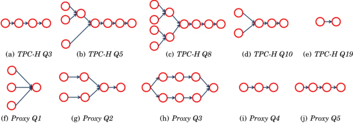
PigMix. We use the well-known PigMix benchmark [Apache 2010] that was created for testing Pig system performance. It consists of 17 Pig programs (L1-L17) and uses datasets generated by the default Pigmix data generator. In total, 1TB of data across 8 tables are generated. The PigMix programs cover a wide range of the Pig features and operators. The data sets are generated with similar properties to Yahoo’s datasets that are commonly processed using Pig. With the exception of L11(that contains a stage with 2 concurrent jobs), the remaining PigMix programs are DAGs of sequential jobs. TPC-H. Our second workload is based on TPC-H [tpc 2008], a standard database benchmark for decision-support workloads. The TPC-H benchmark comes with a data generator that is used to generate the test database for queries included in the TPC-H suite. There are eight tables such as customer, supplier, orders, lineitem, part, part-supp, nation, and region that are used by TPC-H queries. The input dataset size is controlled by the scaling factor (a parameter in the data generator). The scaling factor of 1 generates 1 GB input dataset. The created data is stored in ASCII files where each file contains pipe-delimited load data for the tables defined in the TPC-H database schemas. The Pig system is designed to process a plain text and can load this data easily with its default storage function. We select 5 queries Q3, Q5, Q8, Q10,and Q19 out of 22 SQL queries from the TPC-H benchmark and express them as Pig programs. QueriesQ3 andQ19result in workflows of sequential MapReduce jobs, while the re-maining queries are represented by the DAGs with concurrent MapReduce jobs3_:

(a)TPC-H Q3 (b)TPC-H Q5 (c) TPC-H Q8 (d)TPC-H Q10 (e)TPC-H Q19

(f)Proxy Q1 (g)Proxy Q2 (h) Proxy Q3 (i)Proxy Q4 (j)Proxy Q5 Fig. 2. DAGs of Pig programs in the TPC-H and HP Labs Proxy query sets.

• TheTPC-H Q3retrieves the shipping priority and potential revenue of the orders that had not been shipped and lists them in decreasing order of revenue. It trans-lates into 4 sequential MapReduce jobs with the DAG shown in Figure 2 (a).

• The TPC-H Q5 query lists for each nation in a region the revenue from lineitem transactions in which thecustomerordering parts and thesupplierfilling them are both within that nation. It joins 6 tables, and its dataflow results in 3 concurrent MapReduce jobs. The DAG of the program is shown in Figure 2 (b).

• TheTPC-H Q8query determines how the market share of a givennationwithin a givenregionhas changed over two years for a givenparttype. It joins 8 tables, and its dataflow results in two stages with 4 and 2 concurrent MapReduce jobs respectively. The DAG of the program is shown in Figure 2 (c).

• TheTPC-H Q10query identifies thecustomers, who have returnedpartsthat effect the lost revenue for a given quarter. It joins 4 tables, and its dataflow results in 2 concurrent MapReduce jobs with the DAG of the program shown in Figure 2 (d). • TheTPC-H Q19query reports gross discounted revenue for allordersfor three

dif-ferent types ofpartsthat were shipped by air or delivered in person. It joins 2 tables, and its dataflow results in 2 sequential MapReduce jobs with the DAG of the pro-gram shown in Figure 2 (e).

HP Labs’ Web Proxy Query Set. Our third workload consists of a set of Pig pro-grams for analyzing HP Labs’ web proxy logs. The dataset contains 6 months access logs to web proxy gateway at HP Labs during 2011-2012 years. The total dataset size (12 months) is about 36 GB. There are 438 million records in these logs, The proxy log data contains one record per each web access. The fields include information such as date, time, time-taken, c-ip, cs-host, etc. The log files are stored as plain text and the fields are separated with spaces. Our main intent is to evaluate our models using realistic Pig queries executed on real-world data. We aim to create a diverse set of Pig programs with dataflows with sequential and concurrent jobs.

• TheProxy Q1program investigates the dynamics in access frequencies to different websites per month and compares them across the 6 months. The Pig program re-sults in 6 concurrent MapReduce jobs with the DAG shown in Figure 2 (f).

• The Proxy Q2program aims to discover the co-relationship between two websites from different sets (tables) of popular websites: the first set is created to represent the top 500 popular websites accessed by web users within the HPLabs. The second set contains the top 100 popular websites in US according to Alexa’s statistics4_{. The} DAG of the Pig program is shown in Figure 2 (g).

• The Proxy Q3 program presents the intersect of 100 most popular websites (i.e., websites with highest access frequencies) accessed during the work and after work hours. The DAG of the program is shown in Figure 2 (h).

• Theproxy Q4programs computes the intersection between the top 500 popular web-sites accessed by the HPLabs users and the top 100 popular web-web-sites in US. The program is translated into 3 sequential jobs with the DAG shown in Figure 2 (i). • Theproxy Q5program compares the average daily access frequency for each website

during years 2011 and 2012 respectively. The program is translated into 4 sequential jobs. The DAG of the program is shown in Figure 2 (j).

To perform the validation experiments, we create two different datasets for each of the three workload sets described above:

(1) Atest datasetis used for extracting the job profiles of the corresponding Pig pro-grams.

— PigMix: thetest datasetis generated by the default data generator. It contains 125 million records for the largest table and has a total size around 1 TB. 4_{http://www.alexa.com/topsites}

— TPC-H: the test datasetis generated with scaling factor 9 using the standard data generator. The dataset size is around 9 GB.

— HP Labs’ Web proxy query set: we use the logs from February, March and April as thetest datasetwith the total input size around 18 GB.

(2) Anexperimental datasetis used to validate our performance models using the profiles extracted from the Pig programs that were executed with thetest dataset. Both thetestandexperimentaldatasets are formed by tables with the same layout but with different input sizes.

— PigMix: the input size of the experimental dataset is 20% larger than thetest dataset(with 150 million records for the largest table).

— TPC-H: theexperimental dataset is around 15 GB (scaling factor 15 using the standard data generator).

— HP Labs’ Web proxy query set: we use the logs from May, June and July as the experimental dataset, the total input size is around 18 GB.

4.2. Completion Time Prediction

This section aims to evaluate the accuracy of the proposedbasic performance model, i.e., whether the proposed bound-based model is capable of predicting the completion time of Pig programs as a function of allocated resources.

First, we run the three workloads on the test datasets, and the job profiles of the corresponding Pig programs are built from these executions. By using the extracted job profiles and the designed Pig model, we compute the completion time estimates of Pig programs for processing these two datasets (test and experimental) as a function of allocated resources. Then we validate the predicted completion times against the measured ones. We execute each Pig program three times and report the measured completion time averaged across 3 runs. A standard deviation for most programs in these runs is 1%-2%, with the largest value being around 6%. Since the deviation is so small, we omit the error bars in the figures.

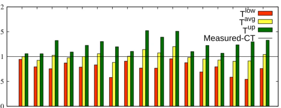
Figure 3 shows the results for the PigMix benchmark that processes thetest dataset when each program in the set is processed with128map and64reduce slots. Given that the completion times of different programs in PigMix are in a broad range of 100s – 2000s, for presentation purposes and easier comparison, wenormalizethe predicted completion times with respect to the measured ones. The three bars in Figure 3 repre-sent the predicted completion times based on the lower (Tlow) and upper (Tup) bounds, and the average of them (Tavg_{). We observe that the actual completion times (shown as} the straightMeasured-CT line) of all 17 programs fall between the lower and upper bound estimates. Moreover, the predicted completion times based on the average of the upper and lower bounds are within 10% of the measured results for most cases. The worst prediction (around 20% error) is for the Pig queryL11. The measured completion time ofL11is very close to the lower bound. Note, that theL11program is the only program in PigMix that is defined by a DAG with concurrent jobs.

Figure 4 shows the results for the PigMix benchmark that processes the experimen-tal datasetwhen each program in the set is processed with64map and64reduce slots. Indeed, our model accurately predicts the program completion time as a function of al-located resources: the actual completion times of all 17 programs are in between the computed lower and upper bounds. The predicted completion times based on the aver-age of the upper and lower bounds provide the best results: 10-12% of the measured results for most cases.

To get a better understanding whether thebasicmodel can accurately predict com-pletion times of Pig programs with concurrent jobs, we perform similar experiments for TPC-H and Proxy queries.

0 0.5 1 1.5 2 L1 L2 L3 L4 L5 L6 L7 L8 L9 L10 L11 L12 L13 L14 L15 L16 L17

Program Completion Time

Tlow Tavg Tup Measured-CT

Fig. 3. Predicted and measured completion time for PigMix executed with test dataset and

128x64slots. 0 0.5 1 1.5 2 2.5 L1 L2 L3 L4 L5 L6 L7 L8 L9 L10 L11 L12 L13 L14 L15 L16 L17

Program Completion Time

Tlow Tavg Tup Measured-CT

Fig. 4. Predicted and measured completion time for PigMix executed withexperimental dataset

and64x64slots. 0 0.5 1 1.5 2 2.5 3 3.5 Q3 Q5 Q8 Q10 Q19

Program Completion Time

Tlow Tavg Tup Measured-CT (a)TPC-H 0 0.5 1 1.5 2 2.5 3 3.5 4 4.5 Q1 Q2 Q3 Q4 Q5

Program Completion Time

Tlow Tavg Tup Measured-CT

(b)Proxy Queries

Fig. 5. Completion time estimates for TPC-H and Proxy queries executed with experimental

datasetand128x64slots.

Figure 5 shows predicted completion times for TPC-H and Proxy queries processed on experimental dataset with128map and64reduce slots. For queries represented by sequential DAGs, such asTPC-H Q3,Q19, andProxy Q4,Q5, thebasicmodel estimates the program completion time accurately and measured results are close to the average bound (within 10%). For queries with concurrent jobs, such as TPC-H Q5, Q10, and Proxy Q2, Q3, the measured completion times are closer to the lower bound, while for queriesTPC-H Q8 andProxy Q1, the measured program completion time is even smaller than the lower bound on the predicted completion time.

Overall, our results show that the proposedbasicmodel provides good estimates for sequential DAGs, but it over-estimates completion times of programs with concurrent jobs, and leads to inaccurate prediction results for these types of Pig programs. In the upcoming Section 5, we will analyze the specifics of concurrent job executions to improve our modeling results.

4.3. Resource Allocation Estimation

Our second set of experiments aims to evaluate the solution of the inverse problem: the accuracy of a resource allocation for a Pig program with a completion time goal, often defined as a part of Service Level Objectives (SLOs).

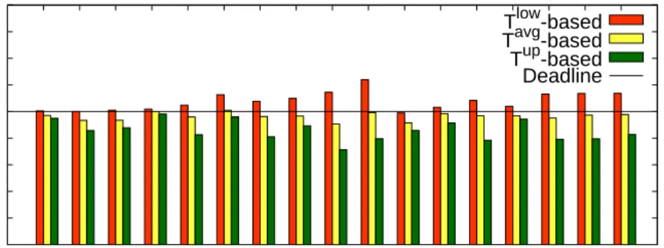
In this set of experiments, letT denote the Pig program completion time when the program is processed with maximum available cluster resources (i.e., when the entire cluster is used for program processing). We set D = 3·T as a completion time goal. Using the Lagrange multipliers’ approach (described in Section 3.3) we compute the required resource allocation, i.e., a fraction of cluster resources, a tailored number of map and reduce slots for the Pig program to be completed with deadline D. As discussed in Section 3.3 we can compute a resource allocation whenD is targeted as either a lower bound, or upper bound or the average of lower and upper bounds on the completion time. Figure 6 shows the measured program completion times based on these three different resource allocations. Similar to earlier results, for presentation purposes, wenormalizethe achieved completion times with respect to deadlineD.

In most cases, the resource allocation that targets D as a lower bound is insuffi-cient for meeting the targeted deadline (e.g., theL17program misses deadline by more than 20%). However, when we compute the resource allocation based onD as an up-per bound – we are always able to meet the required deadline, but in most cases, we over-provision resources, e.g.,L16andL17finish more than 20% earlier than a given deadline. The resource allocations based on the average of lower and upper bounds result in the closest completion time to the targeted program deadlines.

0 0.2 0.4 0.6 0.8 1 1.2 1.4 1.6 1.8 L1 L2 L3 L4 L5 L6 L7 L8 L9 L10 L11 L12 L13 L14 L15 L16 L17

Program Completion Time

Tlow-based Tavg-based Tup-based Deadline

Fig. 6. PigMix executed with theexperimental dataset: do we meet deadlines?

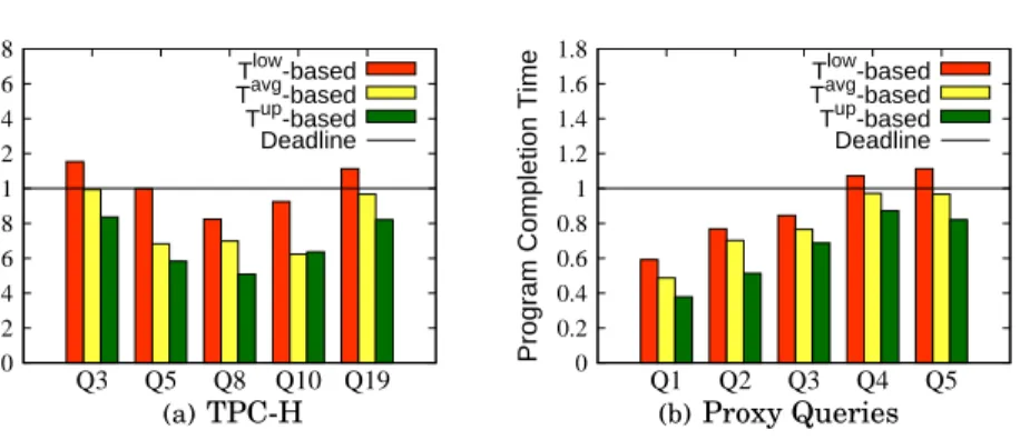
Figure 7 presents similar results for two other workloads: TPC-H and Proxy queries. For queries represented by sequential DAGs, such as TPC-H Q3,Q19, and Proxy Q4,Q5, the resource allocation based on the average bound results is the closest com-pletion time to the targeted program deadlines. However, for programs with concurrent jobs we observe that thebasicmodel is inaccurate. There is a significant resource over-provisioning: the considered Pig programs finish much earlier (up to 50% earlier) than the targeted deadlines.

0 0.2 0.4 0.6 0.8 1 1.2 1.4 1.6 1.8 Q3 Q5 Q8 Q10 Q19

Program Completion Time

Tlow-based Tavg-based Tup-based Deadline (a)TPC-H 0 0.2 0.4 0.6 0.8 1 1.2 1.4 1.6 1.8 Q1 Q2 Q3 Q4 Q5

Program Completion Time

Tlow-based Tavg-based Tup-based Deadline

(b)Proxy Queries

Fig. 7. TPC-H/Proxy queries with theexperimental dataset: do we meet deadlines? In summary, while the basic model produces good results for Pig programs with sequentialDAGs, it over-estimates the completion time of DAGs withconcurrentjobs, and it leads to over-provisioned resource allocations for such programs.

In the next Section 5, we discuss essential differences in performance modeling of concurrent and sequential jobs and offer arefinedmodel.

5. REFINED PERFORMANCE MODEL FOR PIG PROGRAMS

In this section, we analyze the subtleties in execution of concurrent MapReduce jobs and demonstrate that the execution order of concurrent jobs might have a significant impact on the program completion time. We optimize a Pig program execution by en-forcing the optimal schedule of its concurrent jobs, and then introduce an accurate refinedperformance model for Pig programs and their resource allocations.

5.1. Modeling Concurrent Jobs’ Executions

Let us consider two concurrent MapReduce jobsJ1 andJ2. There are no data depen-dencies among the concurrent jobs. Therefore, unlike the execution of sequential jobs where the next job can only start after the previous one is entirely finished (shown in Figure 8 (a)), for concurrent jobs, once the previous job completes its map phase and begins reduce phase processing, the next job can start its map phase execution with the released map resources in a pipelined fashion (shown in Figure 8 (b)). The perfor-mance model should take this “overlap” in executions of concurrent jobs into account. Moreover, this opportunity enables a better resource usage: while one job performs its map tasks processing - the other job may concurrently process their reduce tasks, etc.

J

_J

J

J

_J

J

(a)Sequentialexecution of two jobsJ1andJ2.

J

_J

1R

J

J

_J

2R

J

(b)Concurrentexecution of two jobsJ1andJ2.

Fig. 8. Difference in executions: (a) two sequential MapReduce jobs; (b) two concurrent MapReduce jobs.

Note, that thebasicperformance model proposed in Section 3 approximates the com-pletion time of a Pig programP ={J1, J2}as a sum of completion times ofJ1andJ2 (see eq. 4)independent on whether jobsJ1 andJ2are sequential or concurrent. While such an approach results in straightforward computations, at the same time, if we do not consider possible overlap in execution of map and reduce stages of concurrent jobs then the computed estimates are pessimistic and over-estimate their completion time. We find one more interesting observation about concurrent jobs’ execution of the Pig program. The original Hadoop implementation executes concurrent MapReduce jobs from the same Pig program in a random order. Some ordering may lead to a signif-icantly less efficient resource usage and an increased processing time. Consider the following example with two concurrent MapReduce jobs:

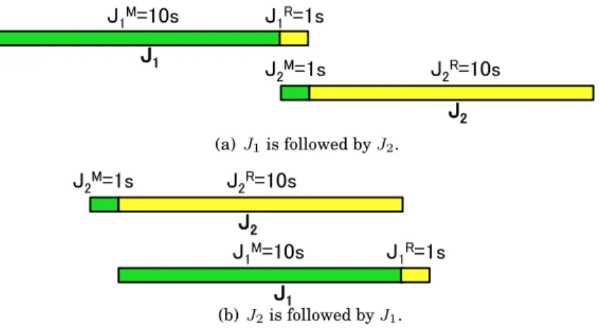
— JobJ1: a map stage durationJ1M = 10sand the reduce stage durationJ R

1 = 1s.

— JobJ2: a map stage durationJ2M = 1sand the reduce stage durationJ2R= 10s. There are two possible executions ofJ1andJ2shown in Figure 9:J1 is followed byJ2 (see Figure 9 a) andJ2is followed byJ1(see Figure 9 b) .

J₁M_{=10s J} 1R=1s J₁ J₂M_{=1s J} 2R=10s J₂ (a)J1is followed byJ2. J₁M_{=10s J} 1R=1s J₁ J₂M_{=1s J} 2R=10s J₂ (b)J2is followed byJ1.

Fig. 9. Impact of concurrent job scheduling on their completion time.

—J1is followed byJ2. The reduce stage ofJ1overlaps with the map stage ofJ2leading to overlap of only1s. The total completion time of processing two jobs is10s+ 1s+

10s= 21s.

—J2is followed byJ1. The reduce stage ofJ2overlaps with the map stage ofJ1leading to a much better pipelined execution and a larger overlap of 10s. The total makespan is1s+ 10s+ 1s= 12s.

There could be a significant difference in the job completion time (75% in the consid-ered example) depending on the execution order of the jobs.

We aim to optimize a Pig program execution by enforcing the optimal schedule of its concurrent jobs. We apply the classic Johnson algorithm for building the optimal two-stage jobs’ schedule [Johnson. 1954]. The optimal execution of concurrent jobs leads to the improved completion time. Moreover, this optimization eliminates possible non-determinism in Pig program execution, and enables more accurate completion time predictions for Pig programs.

5.2. Completion Time Estimates for Pig Programs with Concurrent Jobs

Let us consider a Pig programP that is compiled into a DAG of MapReduce jobs. This DAG represents the Pig program execution plan. The Pig engine partitions the DAG into multiple stages, where each stage contains one or more independent MapReduce jobs which can be executed concurrently. For a plan execution, the Pig system first submits all the jobs from the first stage. Once they are completed, it submits jobs from the second stage, etc. This process continues until all the jobs are completed.

Note that due to the data dependencies in a Pig execution plan, thenext stagecannot start until theprevious stagefinishes. Thus, the completion of a Pig programP which containsSstagescan be estimated as follows:

TP =

X

1≤i≤S

TSi (6)

whereTSi represents the completion time of stagei.

For a stage that consists of a single jobJ, the stage completion time is defined by the jobJ’s completion time. For a stage that contains concurrent jobs, the stage completion time depends on the jobs’ execution order.

Suppose there are |Si| jobs within a particular stageSi and the jobs are executed according to the order{J1, J2, ...J|Si|}. Note, that given a number of map/reduce slots

(SP

M, SRP), we can estimate the durations of map and reduce phases of MapReduce jobs

Ji(1 ≤ i ≤ |Si|). These map and reduce phase durations are required by the John-son’s algorithm [Johnson. 1954] to determine the optimal schedule of jobs in the set {J1, J2, ...J|Si|}.

Let us assume, that for each stage with concurrent jobs, we have already determined the optimal job schedule that minimizes the completion time of the stage. Now, we introduce therefinedperformance model for predicting the Pig programP completion timeTP as a function of allocated resources(SMP, S

P

R). We use the following notations:

timeStartM

Ji the start time of jobJi’s map phase

timeEndM

Ji the end time of jobJi’s map phase

timeStartR

Ji the start time of jobJi’s reduce phase

timeEndR

Ji the end time of jobJi’s reduce phase

Then the stage completion time can be estimated as TSi =timeEnd

R

J|Si|−timeStart M

J1 (7)

We now explain how to estimate the start/end time of each job’s map/reduce phase5_. Let TM

Ji and T

R

Ji denote the completion times of map and reduce phases of job Ji

respectively. We can compute phase duration as a function of allocated map/reduce slots(S_MP, S_RP), e.g., using a lower or upper bound estimates as described in Section 2. For the rest of the paper, we use the completion time estimates based on the average of the lower and upper bounds. Then

timeEndM_Ji =timeStartM_Ji +T_JM_i (8) timeEndR_J i =timeStart R Ji+T R Ji (9)

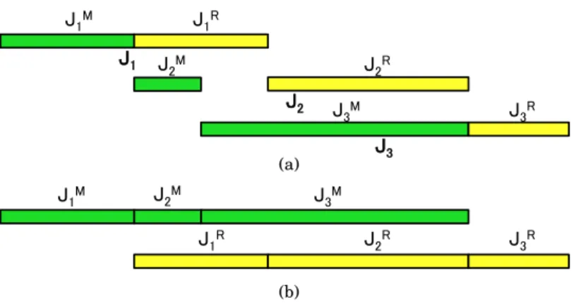
Figure 10 shows an example of three concurrent jobs execution in the orderJ1, J2, J3.

5_{These computations present the main, typical case when the number of allocated slots is smaller than the number of tasks} that jobs need to process, and therefore, the execution of concurrent jobs is pipelined. There are some corner cases with small concurrent jobs when there are enough resources for processing them at the same time. In this case, the designed model over-estimates the stage completion time. We have an additional set of equations that describes these corner cases in a more accurate way. We omit them here for a presentation simplicity.

J₁M _J 1R J_{1 J} 2M J2R J_{2 J} 3M J3R J₃ (a) J₁M J₁R J₂M J₂R J₃M J₃R (b)

Fig. 10. Execution of Concurrent Jobs

Note, that Figure 10 (a) can be rearranged to show the execution of jobs’ map/reduce stages separately (over the map/reduce slots) as shown in Figure 10 (b). It is easy to see that since all the concurrent jobs are independent, the map phase of the next job can start immediately ones the previous job’s map stage is finished, i.e.,

timeStartMJi =timeEnd M Ji−1=timeStart M Ji−1+T M Ji−1 (10)

The start timetimeStartR_Ji of the reduce stage of the concurrent jobJi should satisfy the following two conditions:

(1) timeStartR_J i ≥timeEnd M Ji (2) timeStartR Ji ≥timeEnd R Ji−1

Therefore, we have the following equation: timeStartR_J i=max{timeEnd M Ji, timeEnd R Ji−1}= =max{timeStartM Ji +T M Ji, timeStart R Ji−1+T R Ji−1} (11)

Then the completion time of the entire Pig programP is defined as thesum of its stagesusing eq. (6). This approach offers arefinedperformance model for Pig programs. 5.3. Resource Allocation Estimates for Optimized Pig Programs

Let us consider a Pig programP with a given deadlineD. The optimized execution of concurrent jobs inP may significantly improve the program completion time. There-fore, P may need to be assigned a smaller amount of resources for meeting a given deadlineD compared to its non-optimized execution. As shown in Section 4, the ear-lier proposed basicmodel over-estimates the completion time for Pig programs with concurrent jobs. However, the unique benefit of this model is that it allows to express the completion timeDof a Pig program via a special form equation shown below:

D= A P SP M +A P SP R +CP (12)

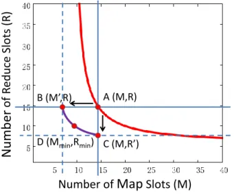
whereS_MP andS_RP denote the number of map and reduce slots assigned toP. Eq. (12) can be used for solving the inverse problem of finding the resource allocation (S_MP, S_RP) such that Pig programP completes within timeD. This equation yields a hyperbola if S_MJ andS_RJ are considered as variables. We can directly calculate the minima on this curve using Lagrange’s multipliers (see Section 3.1).

The refined model introduced in the previous Section 5.2 for predicting the com-pletion time of an optimized Pig program is more complex. It requires computing a functionmaxfor stages with concurrent jobs, and therefore, it cannot be expressed as a single equation for solving the inverse problem. However, we can use the “over-sized” resource allocation defined by the basic modeland eq. (12) as an initial point for de-termining the solution required by the optimized Pig programP. The hyperbola with all the possible solutions according to thebasicmodel is shown in Figure 11 as the red curve, and A(M, R) represents the point with a minimal number of map and reduce slots (i.e., the pair(M, R)results in the minimal sum of map and reduce slots).

B (M’,R)

A (M,R)

D (M

,R

) C (M,R’)

Nu

mb

er

of

R

educe S

lots (

R)

Number of

Map

Slots (M)

Fig. 11. Resource allocation estimates for an optimized Pig program.

Algorithm 1 described below shows the computation for determining the minimal resource allocation pair (Mmin, Rmin)for an optimized Pig programP with deadline D. This computation is illustrated by Figure 11.

First, we find the minimal number of map slotsM0 (i.e., the pair(M0, R)) such that deadline D can still be met by the optimized Pig program with the enforced optimal execution of its concurrent jobs. We do it by fixing the number of reduce slots to R, and then step-by-step reducing the allocation of map slots. Specifically, Algorithm 1 sets the resource allocation to (M −1, R)and checks whether programP can still be completed within time D (we useT_Pavg for completion time estimates). If the answer is positive, then it tries(M−2, R)as the next allocation. This process continues until pointB(M0, R)(see Figure 11) is found such that the numberM0 of map slots cannot be further reduced for meeting a given deadlineD(lines 1-4 of Algorithm 1).

At the second step, we apply the same process for finding the minimal number of reduce slotsR0(i.e., the pair(M, R0)) such that the deadlineDcan still be met by the optimized Pig programP (lines 5-7 of Algorithm 1).

At the third step, we determine the intermediate values on the curve between (M0, R) and (M, R0) such that deadline D is met by the optimized Pig program P. Starting from point(M0, R), we are trying to find the allocation of map slots fromM0 to M, such that the minimal number of reduce slots Rˆ should be assigned toP for meeting its deadline (lines 10-12 of Algorithm 1).

Finally, (Mmin, Rmin)is the pair on this curve such that it results in the minimal sum of map and reduce slots.

ALGORITHM 1:Determining the resource allocation for a Pig program

Input: Job profiles of all the jobs inP ={J1, J2, ...J|Si|}

D←a given deadline

(M, R)←the minimum pair of map and reduce slots obtained forPand deadlineDby applying thebasicmodel

Optimal execution of jobsJ1, J2, ...J|S_i|based on(M, R)

Output: Resource allocation pair(Mmin, Rmin)for optimizedP

1 M0←M,R0←R;

2 whileT_Pavg(M0, R)≤D // From A to B

3 do

4 M0⇐M0−1;

5 end

6 whileT_Pavg(M, R0)≤D // From A to C

7 do

8 R0⇐R0−1; 9 end

10 Mmin←M, Rmin←R,M in←(M+R);

11 forMˆ ←M0+ 1toM // Explore blue curve B to C 12 do 13 Rˆ=R−1; 14 whileT_Pavg( ˆM ,Rˆ)≤Ddo 15 Rˆ⇐Rˆ−1; 16 ifMˆ + ˆR < M inthen 17 Mmin⇐M , Rˆ min⇐R, M inˆ ←( ˆM+ ˆR); 18 end 19 end 20 end

6. EVALUATION OF THE REFINED MODEL

In this section, we evaluate performance benefits of introduced optimized executions of Pig programs with concurrent jobs. Then, we assess the accuracy of the proposed refinedperformance model for completion time estimates and resource allocation deci-sions for Pig programs.

In the evaluation study, we consider the programs with concurrent jobs in two work-loads:TPC-H andProxy queries. We do not present results ofPigMixbenchmark be-cause only 1 of 17 Pig programs included in the benchmark contains concurrent jobs. We perform the experiments using our 66 node Hadoop cluster with the same configu-ration as described in Section 4.

6.1. Optimal Schedule of Concurrent Jobs

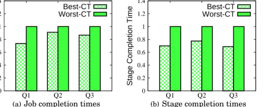
Figures 12 and 13 show the scheduling impact of concurrent jobs on the program com-pletion time for three TPC-H queriesQ5, Q8, and Q10 andProxy queriesQ1, Q2, and Q3 respectively when each program in those sets is processed with 128map and64 reduce slots. Figures 12 (a) and 13 (a) show two extreme measurements: the best pro-gram completion time (i.e., when the optimal schedule of concurrent jobs is chosen) and the worst one (i.e., when concurrent jobs are executed in the “worst” possible or-der based on our estimates). For presentation purposes, the best (optimal) completion time isnormalizedwith respect to the worst one. The choice of optimal schedule of concurrent jobs reduces the completion time by 10%-27% compared with the worst case ordering. Figures 12 (b) and 13 (b) show completion times of stages with

0 0.2 0.4 0.6 0.8 1 1.2 1.4 Q5 Q8 Q10

Program Completion Time

Best-CT Worst-CT

(a)Job completion times

0 0.2 0.4 0.6 0.8 1 1.2 1.4 Q5 Q8 Q10

Stage Completion Time

Best-CT Worst-CT

(b)Stage completion times

Fig. 12. Measured (normalized) completion times for different schedules of concurrent jobs in TPC-H queries. 0 0.2 0.4 0.6 0.8 1 1.2 1.4 Q1 Q2 Q3

Program Completion Time

Best-CT Worst-CT

(a)Job completion times

0 0.2 0.4 0.6 0.8 1 1.2 1.4 Q1 Q2 Q3

Stage Completion Time

Best-CT Worst-CT

(b)Stage completion times

Fig. 13. Measured (normalized) completion times for different schedules of concurrent jobs in Proxy queries.

current jobs under different schedules for the same TPC-H and Proxy queries. The performance benefits at the stage level are even higher: they range between 20%-30%. 6.2. Predicting the Completion Time

Figure 14 shows the Pig program completion time estimates based on the earlier intro-ducedbasicmodel and and the newrefinedmodel forTPC-HandProxy queriesdefined by the DAGs with concurrent jobs. The completion time estimates are computed us-ingT_Pavg (the average of the lower and upper bounds). The programs are executed on theexperimentaldataset. Figures 14 and 15 shows the results for the case when each program is processed with128x64and32x64map and reduce slots respectively.

The completion time estimates based on the newrefinedmodel are significantly im-proved compared to the basicmodel results which are too pessimistic. In most cases (11 out of 12), the predicted completion time is within 10% of the measured ones. 6.3. Estimating Resource Allocations with Refined Model

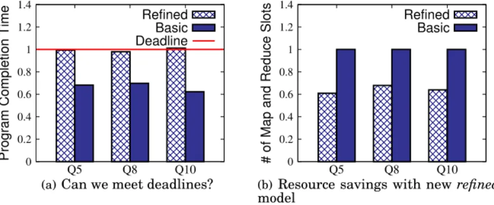
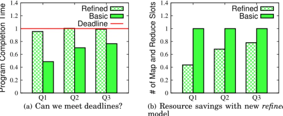
In this set of experiments, let T denote the Pig program completion time when pro-gramP is processed with maximum available cluster resources. We setD= 2·T as a completion time goal. Then we compute the required resource allocation forP whenD is targeted asT_Pavg, i.e., the average of lower and upper bounds on the completion time. Figures 16 (a) and 17 (a) compare the measured completion times achieved by the TPC-H and Proxy’squeries respectively when they are assigned the resource alloca-tions computed with the basicversus refinedmodels. The completion times are nor-malizedwith respect to the targeted deadlines. While both models suggest sufficient resource allocations that enable the considered queries to meet their deadlines, the ba-sic model significantly over-provisions resources, and the queries finish much earlier

0 0.5 1 1.5 2 2.5 Q5 Q8 Q10

Program Completion Time

CT-Predicted-Refined-Model CT-Predicted-Basic-Model Measured-CT (a)TPC-H 0 0.5 1 1.5 2 2.5 Q1 Q2 Q3

Program Completion Time

CT-Predicted-Refined-Model CT-Predicted-Basic-Model Measured-CT

(b)Proxy’s Queries

Fig. 14. Predicted completion times usingbasicvsrefinedmodels (128x64slots) with the exper-imental dataset.. 0 0.5 1 1.5 2 2.5 Q5 Q8 Q10

Program Completion Time

CT-Predicted-Refined-Model CT-Predicted-Basic-Model Measured-CT (a)TPC-H 0 0.5 1 1.5 2 2.5 Q1 Q2 Q3

Program Completion Time

CT-Predicted-Refined-Model CT-Predicted-Basic-Model Measured-CT

(b)Proxy’s Queries

Fig. 15. Predicted completion times usingbasicvsrefinedmodels (32x64slots) with the experi-mental dataset. .

(55%-20% earlier) than given deadlines. The resource allocations computed with the refinedmodel are much more accurate, and all the queries complete within 10% of the targeted deadlines. 0 0.2 0.4 0.6 0.8 1 1.2 1.4 Q5 Q8 Q10

Program Completion Time

Refined Basic Deadline

(a)Can we meet deadlines?

0 0.2 0.4 0.6 0.8 1 1.2 1.4 Q5 Q8 Q10

# of Map and Reduce Slots

Refined Basic

(b)Resource savings with newrefined model

Fig. 16. TPC-H Queries: efficiency of resource allocations with newrefinedmodel.

Figures 16 (b) and 17 (b) compare the amount of resources (the sum of map and re-duce slots) computed with thebasicmodel versusrefinedmodel forTPC-HandProxy’s queriesrespectively. Therefinedmodel is able to achieve targeted deadlines with much

0 0.2 0.4 0.6 0.8 1 1.2 1.4 Q1 Q2 Q3

Program Completion Time

Refined Basic Deadline

(a)Can we meet deadlines?

0 0.2 0.4 0.6 0.8 1 1.2 1.4 Q1 Q2 Q3

# of Map and Reduce Slots

Refined Basic

(b)Resource savings with newrefined model

Fig. 17. Proxy’s Queries: efficiency of resource allocations with newrefinedmodel. smaller resource allocations (20%-60% smaller) compared to resource allocations sug-gested by thebasicmodel. Therefore, the proposed optimal schedule of concurrent jobs combined with the accurate refinedperformance model lead to the efficient execution and significant resource savings for deadline-driven Pig programs.

7. DISCUSSION AND FUTURE WORK

In designing our modeling framework, we exploit the fact that a typical production Hadoop (Pig) job is executed routinely on new data. We take advantage of this obser-vation, and for a periodic Pig program, we automatically build its jobs’ profiles from the past execution. These extracted job profiles are used forfuturepredictions when this Pig program is executed on new data. The question is how sensitive the model and the prediction results to a given training data (i.e. to the extracted job profile from the last job execution). If the amount of new data is close in size (e.g.,±20%) to the data processed in the past (when the Pig jobs’ profiles were built) then the proposed models work well and they are accurate. Most of our predictions are within 10%-15% of the measured results.

However, if the Pig program processes a significantly different amount of data (e.g., twice as much) compared to the past execution when the job profiles were built – how does it impact the accuracy of our models and their predictions?

In our profiling approach, we estimate processing costs per record during different execution stages: map, shuffle/sort, and reduce phases. This normalized cost is used to project the map/reduce task duration when these tasks need to process the increased (or decreased) amounts of data (records). Figure 18 (a) shows a predicted completion time (normalized with respect to the measured time) ofTPC-H Q10with different scale factors. Our prediction is based on the job profiles extracted fromTPC-H Q10with the scale factor 9.

Using these job profiles we predictTavgforTPC-H Q10based on different scale fac-tors. The predicted results are accurate for scale factors 10,15, 20, and still acceptable for scale factor 7. The prediction errors for scale factors 3 and 5 are significantly higher. To understand the logic behind these results, we analyze TPC-H Q10 processing in more detail (see its DAG in Figure 2 (c)). Our measurements reveal that the first stage is responsible for 40% of the overall execution time. Therefore, analyzing the profiles of two concurrent jobsJ1andJ2of this stage will be very useful. Figures 18 (b) and (c) show the processing costs per record during different execution phases ofJ1andJ2 re-spectively. Apparently, the job profiles are quite stable starting at the scale factor 8 and up. It explains why the completion time predictions for these scale factors are accurate. However, for small scale factors, the processing costs per record, especially in reduce

0 0.2 0.4 0.6 0.8 1 1.2 1.4 3 5 7 9 10 15 20

Program Completion Time

Scale Factor

T

Measured-CT

(a)Completion time estimates

0 0.02 0.04 0.06 0.08 0.1 0.12 1 2 3 4 5 6 7 8 9 10 15 20

Per Record Cost (ms)

Scale Factor Avg-Map Avg-Reduce Avg-Shuffle Max-Map Max-Reduce Max-Shuffle

(b)Job profiles for Q10-1-1

0 0.005 0.01 0.015 0.02 0.025 0.03 0.035 1 2 3 4 5 6 7 8 9 10 15 20

Per Record Cost (ms)

Scale Factor Avg-Map Avg-Reduce Avg-Shuffle Max-Map Max-Reduce Max-Shuffle

(c)Job profiles for Q10-1-2

Fig. 18. Completion time estimates forTPC-H Q10with different input data size (scale factor).

and shuffle phases, are significantly higher. There is an overhead associated with a task execution and it contributes a significant portion in the task duration when pro-cessing a small set of records. The overhead impact is significantly diminished when processing a larger dataset, and the cost per record becomes more representative of the actual processing cost.

In our future work, we plan to investigate these overheads in more detail to take them into account for computing the per record cost and in scaling the job profiles for different amount of input data. The other interesting alternative is to derive (and interpolate) the per record cost empirically using the available set of past runs of the Pig program on datasets of different sizes.

The other related issue is the impact of resource contention on the Pig program com-pletion time when multiple Pig programs or MapReduce jobs are executed simultane-ously. Even when a Pig program is executed on the Hadoop cluster in isolation there is an inevitable resource contention because there are multiple slots at each worker node, and the different tasks of the same job scheduled on these slots compete for the shared node resources. These tasks compete for the disk i/o and the network resources in a similar way as the tasks of different jobs. When the designed performance models become a part of the SLO-based scheduler [Verma et al. 2011a], there is an additional scheduler feature that can increase or decrease the number of slots allocated to a job based on the expected progress of this job. This additional scheduler feature aims to compensate the possible model inaccuracy due to resource contention or unforeseen ex-ecutional runtime non-determinism, and in such a way improve the overall scheduler outcome.

8. RELATED WORK

While performance modeling in the MapReduce framework is a new topic, there are several interesting research efforts in this direction.

Polo et al. [Polo et al. 2010] introduce an online job completion time estimator which can be used in their new Hadoop scheduler for adjusting the resource allocations of different jobs. However, their estimator tracks the progress of the map stage alone, and use a simplistic way for predicting the job completion time, while skipping the shuffle/sort phase, and have no information or control over the reduce stage.

FLEX [Wolf et al. 2010] develops a novel Hadoop scheduler by proposing a special slot allocation schema that aims to optimize some given scheduling metric. FLEX relies on the speedup function of the job (for map and reduce stages) that defines the job execution time as a function of allocated slots. However, it is not clear how to derive this function for different applications and for different sizes of input datasets. The authors do not provide a detailed MapReduce performance model for jobs with targeted job deadlines.

ARIA[Verma et al. 2011a] introduces a deadline-based scheduler for Hadoop. This scheduler extracts and utilizes the job profiles from the past executions, and provides a variety of bounds-based models for predicting a job completion time as a function of allocated resources and a solution of the inverse problem. The shortcoming of this work is that it does not have scaling factors to adjust the extracted profile when the job is executed on a different size dataset. In the follow up work [Verma et al. 2011b], a more general profiling approach that is based on regression technique for deriving the scaling factors is proposed. However, these models apply to a single MapReduce job.

Tian and Chen [Tian and Chen ] aim to predict performance of a single MapReduce program from the test runs with a smaller number of nodes. They consider MapRe-duce processing at a fine granularity. For example, the map task is partitioned in 4 functions: read a block, map function processing of the block, partition and sort of the processed data, and the combiner step (if it is used). The reduce task is decomposed in 4 functions as well. The authors use alinear regression techniqueto approximate the cost (duration) of each function. These functions are used for predicting the larger dataset processing. There are a few simplifying assumptions, e.g., a single wave in the reduce stage. The problem of finding resource allocations that support given job completion goals are formulated as an optimization problem that can be solved with existing commercial solvers.

There is an interesting group of papers that design a detailed job profiling ap-proach for pursuing a different goal: to optimize the configuration parameters of both a Hadoop cluster and a given MapReduce job (or workflow of jobs) for achieving the im-proved completion time.Starfishproject [Herodotou et al. 2011; Herodotou and Babu 2011] applies dynamic instrumentation to collect a detailed run-time monitoring in-formation about job execution at a fine granularity: data reading, map processing, spilling, merging, shuffling, sorting, reduce processing and writing. Such a detailed job profiling information enables the authors to analyze and predict job execution under different configuration parameters, and automatically derive an optimized configura-tion. One of the main challenges outlined by the authors is a design of an efficient searching strategy through the high-dimensional space of parameter values. The au-thors offer a workflow-aware scheduler that correlate data (block) placement with task scheduling to optimize the workflow completion time. In our work, we propose comple-mentary optimizations based on optimal scheduling of concurrent jobs within the DAG to minimize overall completion time.

Kambatla et al [Kambatla et al. 2009] propose a different approach for optimizing the Hadoop configuration parameters (number of map and reduce slots per node) to