Causal Discovery Using A Bayesian Local Causal Discovery Algorithm

Amsterdam: IOS Press

© 2004 IMIA. All rights reserved

Causal Discovery Using A Bayesian Local Causal Discovery Algorithm

Subramani Mani

, Gregory F. Cooper

[email protected] [email protected]

a _{Center for Biomedical Informatics and the Intelligent Systems Program, University of Pittsburgh PA 15213} b _{Department of Computer Science, University of Wisconsin-Milwaukee, Milwaukee WI 53201}

Subramani Mani, Gregory F. Cooper

This study focused on the development and application of an ef-ficient algorithm to induce causal relationships from observa-tional data. The algorithm, called BLCD, is based on a causal Bayesian network framework. BLCD initially uses heuristic greedy search to derive the Markov Blanket (MB) of a node that serves as the “locality” for the identification of pair-wise causal relationships. BLCD takes as input a dataset and outputs poten-tial causes of the form variable X causally influences variable Y. Identification of the causal factors of diseases and outcomes, can help formulate better management, prevention and control strategies for the improvement of health care. In this study we fo-cused on investigating factors that may contribute causally to in-fant mortality in the United States. We used the U.S. Linked Birth/Infant Death dataset for 1991 with more than four million records and about 200 variables for each record. Our sample consisted of 41,155 records randomly selected from the whole dataset. Each record had maternal, paternal and child factors and the outcome at the end of the first year—whether the infant survived or not. Using the infant birth and death dataset as in-put, BLCD output six purported causal relationships. Three out of the six relationships seem plausible. Even though we have not yet discovered a clinically novel causal link, we plan to look for novel causal pathways using the full sample.

Keywords:

Causal Discovery, Infant Mortality, Bayesian Networks

Introduction

Causal discovery is a challenging and important task. Causal knowledge aids planning and decision making in almost all fields. For example, in the domain of medicine, determining the cause of a disease helps in prevention and treatment.

Well-designed experimental studies, such as randomized con-trolled trials, are typically employed in assessing causal relation-ships. Here the value of the variable postulated to be causal is set randomly and its effects measured. These studies are appro-priate in certain situations, for example, animal studies and stud-ies involving human subjects that have undergone a thorough procedural and ethical review. Experimental studies may not, however, be feasible in many contexts due to ethical, logistical, or cost considerations. These practical limitations of experimen-tal studies heighten the importance of exploring, evaluating and

refining techniques to learn more about causal relationships from observational data, as for example data routinely collected in astronomy, earth sciences and healthcare. The aim is not to replace experimental studies, which are extremely valuable in science, but to complement experimental studies when feasible. This paper introduces a new Bayesian local causal discovery al-gorithm called BLCD that is designed for efficient discovery of possible causal relationships from large observational databases. The time complexity of BLCD makes it appropriate for explor-ing possible causal relationships in databases that contain a very large number of records (on the order of hundreds of thousands) and a moderately large number of measured variables per record (on the order of hundreds).

In our study using BLCD we focus on investigating factors that may contribute causally to infant mortality in the United States. Infant mortality is one of the most important public health prob-lems in the U.S. [1]. International comparisons based on data from the United Nations statistical office for the year 1991 show that there are 21 countries in the world with lower infant mortal-ity rates than the United States. Japan had the lowest rate of 4.4, while the US rate was 8.9 [2]. The present study is a prelude to further work using larger real-world medical and biological datasets.

Materials and Methods

Assumptions for Causal Discovery

In the research reported here, we use causal Bayesian networks to represent causal relationships among model variables. This section provides a brief introduction to causal Bayesian net-Figure 1 - A hypothetical causal Bayesian network structure

works, as well as a description of the assumptions we used to ap-ply these networks for causal discovery.

A causal Bayesian network (CBN) is a Bayesian network in which each arc is interpreted as a direct causal influence between a parent node (variable) and a child node, relative to the other nodes in the network [3]. Figure illustrates the structure of a hy-pothetical causal Bayesian network structure, which contains five nodes. The causal network structure in Figure indicates, for example, that a History of Smoking can causally influence whether Lung Cancer is present, which in turn can causally in-fluence whether a patient experiences Fatigue or presents with a Mass Seen on Chest X-ray.

The causal Markov condition gives the independence relation-ships that are specified by a causal Bayesian network:

A variable is independent of its non-descendants (i.e., non-effects) given just its parents (i.e., its direct causes). According to the Markov condition, the causal network is rep-resenting that the chance of a Mass Seen on Chest X-ray will be independent of a History of Smoking, given that we know wheth-er Lung Cancwheth-er is present or not. While the causal Markov con-dition specifies independence relationships among variables, the

causal faithfulness condition specifies dependence relation-ships:

Variables are independent only if their independence is implied by the causal Markov condition.

For the causal network structure in Figure three examples of the causal faithfulness condition are (1) History of Smoking and Lung Cancer are probabilistically dependent, (2) History of Smoking and Mass Seen on Chest X-ray are dependent, and (3) Mass Seen on Chest X-ray and Fatigue are dependent. The intu-ition behind that last example is as follows: a Mass Seen on Chest X-ray increases the chance of Lung Cancer which in turn increases the chance of Fatigue; thus, the variables Mass Seen on Chest X-ray and Fatigue are expected to be probabilistically de-pendent. In other words, the two variables are dependent be-cause of a common be-cause (i.e., a confounder). The causal Markov and faithfulness conditions describe probabilistic inde-pendence and deinde-pendence relationships, respectively, that are represented by a CBN.

Before we move on to the next property of a CBN, we introduce our notational convention. Sets of variables are represented in bold and upper case, random variables by upper case letters ital-icized and lower case letters will be used to represent the value of a variable or sets of variables. When we say X = x, we mean an instantiation of all the variables in X, while X=x denotes that the variable X is assigned the value x. Graphs are denoted by a bold italicized G.

BLCD: A Bayesian Local Causal Discovery Algorithm

We introduce a Bayesian local causal discovery algorithm (BLCD) that conjectures causal relationships between pairs of

variables that have no common causes (confounders). Instead of using constraint-based independence and dependence tests, we score the models by a Bayesian method. This confers the follow-ing advantages:

1. Allows informative causal priors to be incorporated. 2. Provides a quantitative posterior assessment of causality,

based on prior belief and data. BLCD assumes the following:

Assumption 1: The causal Markov condition

Assumption 2: The causal faithfulness condition X → Y (1) X ← Y (2)

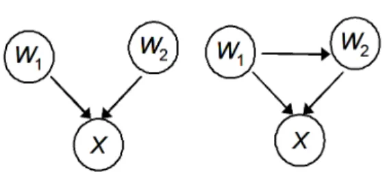
Figure 2 - Two independence-equivalent BNs.

We now introduce the concept of independence equivalence. Consider two Bayesian network structures Bs1 and Bs2. Bs1 and Bs2 are said to be independence equivalent if they represent the same conditional independence assertions for V, where V is the set of variables in Bs1 and Bs2 [4]. The two network structures in Figure 4 are independence equivalent. In particular they rep-resent no conditional independence assertion. Likewise, all the three network structures in Figure 5 are also independence equivalent asserting that X and Z are conditionally independent given Y. Two network structures are independence equivalent if and only if they have the same “V” structures and also share oth-er edges (ignoring directions) that are not part of a “V” [5]. A “V” structure involving variables W1, W2 and X is shown in Figure 4. There is a directed edge from W1 to X and another di-rected edge from W2 to X. There is no edge between W1 and W2. A “V” structure contains a “collider”; the node X is a collid-er. Since W1 and W2 are marginally independent, X is also termed an unshielded collider. Figure shows a model in which W1 and W2 are dependent and where X is a shielded collider. BLCD requires that a node X be an unshielded collider in order to discover the causal effects of X.

Using the BLCD search strategy, for each pair of nodes X and Y where X is a collider, the probability of XY will be derived under assumptions. We illustrate this first using a hypothetical domain with four discrete random observed variables — W1, W2, X, and Y (see Figure 6). The model G1 has the “Y” structure format. A “Y” structure is required in BLCD to infer pairwise causal rela-tionships in an unconfounded way from observational data mak-ing just the two basic assumptions (causal Markov and causal faithfulness) for causal discovery.

X → Y → Z (1) X ← Y ← Z (2) X ← Y → Z (3)

Figure 3 - Three independence-equivalent BNs Figure 6 also shows models G2 and G3, from our four variable domain. The 3 models shown are a small subset of the 543 po-tential CBN models for a four variable domain.

.

The following equation is used in BLCD to approximate the probability of an unconfounded causal relationship X→Y:

The above scoring function assigns relative scores to the models that represent the probability of the model given data and prior knowledge. The scoring can be done, for example, using a Bayesian metric such as the K2 metric [6] or the BDe metric [7]. Our implementation of the scoring function uses the BDe metric with uniform parameter and structure priors.

The 543 structures cover the space of CBN models exhaustively and no other structure has the same depend ence/independence properties as G1, i.e., there is no other CBN in the four node do-main in the independence equivalent class of G1. In the large sample limit the posterior probability of G1 will approach 1.0 relative to the other 542 models if indeed (1) X causally influ-ences Y in an unconfounded manner, (2) X is a collider of W1 and W2 in the distribution of the causal process generating the data, and (3) the Markov and Faithfulness conditions hold. Equa-tion 1 serves as a lower bound on X→Y, relative to considering only the 543 CBN structures on four variables. Equation 1 does not, however, model latent variables, and thus, it is only a heu-ristic Bayesian score. We are giving up a full Bayesian treatment of the problem in order to gain computational efficiency. The heuristic methodology to select the tetrasets (W1, W2, X and Y) is given below. The method involves identification of the Markov Blanket of each random variable. The Markov Blanket (MB) of a node X in a CBN G is the union of the set of parents of X, the children of X, and the parents of the children of X [4]. Note that it is the minimal set of nodes when conditioned on

(in-stantiated) that ensures that a node X will be independent of all the other nodes in the CBN. Let V be the set of all variables in G, B the MB of X, and A be V \ (B»X). Conditioning on B ren-ders X independent of A. For example, in the hypothetical CBN shown in Figure , the MB of node v4 is composed of v2 and v3; the MB of node v2 is v1, v3, and v4.

We derive the MB of a node (designated as B) by a greedy heu-ristic search and refer to it as the Procedure MB. The set B ⊆ (V \ X) that maximizes the score for the structure BX based on a greedy forward search as described in [6] is initially identified. This is followed by a one step backward greedy search that prunes B to yield set B ⊆ B that maximizes the score for the structure BX.This set B is updated using the following rule: If X is in the MB of Y, but Y is not in the MB of X, add Y to the MB of X. We refer to this rule as the MB update rule.

BLCD steps

1. Derive the Markov Blanket: For each node X∈X, heu-ristically derive the Markov Blanket of X using the Pro-cedure MB. X denotes the set of all random observed variables in the dataset. Let B denote the MB of X. 2. Update B: Apply the MB update rule.

3. Pick W1, W2, X and Y: Select sets of four variables from the set obtained by the union of B and X as follows. We refer to each set of four variables as a tetraset T. Since we are focusing on the MB of X, X is an essential ele-ment of T. Note that each tetraset can give rise to 3 “Y” patterns where the X variable is a cause and each of the other three are potential effects.

4. Derive P(X→Y | D): For each of the 3 “Y” patterns, the probability of XY is derived using Equation 1.

5. Generate output: If P(X→Y | D) > t, where t is a user-set threshold, then output X→Y.

By setting t close to 1.0, we avoid generating many false posi-tives, which is one of our key goals. In causal datamining we do not want to overwhelm the user with many false positives. We would like to trade off recall (number of true causal relationships output over the total number of true causal relationships) for pre-cision or positive predictive value (number of true causal rela-tionships over the total number of relarela-tionships output). In other words we want to improve the signal to noise ratio in the output and the goal is to pick just the signals (true causal relationships). BLCD can be implemented in an anytime framework, to output the purported causes as they are found. To discover the effects of a node X, we require only the MB of X and data on X and the vari-ables in the MB of X.

Related work

A review of the philosophical literature on causality is beyond the scope of this paper. For a detailed discussion of the relation-ship between statistical association and causation, including philosophical issues, see for example [8] and [9].

Constraint-based approaches to causal discovery were put for-ward by Pearl and Verma [10] and by Spirtes, Glymour, and Scheines [11]. The PC and FCI algorithms, for instance, take a global approach to causal discovery and output a graph with dif-ferent types of edges between all the variables to represent for Figure 4- A «V» structure Figure 5- A «Shielded» collider

Figure 4 - Three causal models that contain four nodes out of the possible 543 models. G1 has a “Y” pattern.

P X( →Y D) Score G( 1D) Score G( ₁ D) i=1 543

∑

example that X causes Y, X does not cause Y, or the causal direc-tion is undetermined [12]. The FCI algorithm can also model la-tent variable patterns.

Earlier research on learning Bayesian networks from data using a Bayesian approach [6,7] has simultaneously modeled all the causal relationships among the model variables. These global approaches can require long search times when the number of variables is large. When they are used to model latent variables, these approaches can be extremely slow, even when modeling only a few variables.

LCD [13] and its variants [14] output causes of the form X causes Y and take a local and constraint-based approach to causal dis-covery (evaluate only triplets of the form WXY). By searching only for pairwise causal relationships, they trade off complete-ness for efficiency. They also need background knowledge in the form of instrumental variable(s). Silverstein and others have used a variant of LCD to perform market basket analysis to dis-cover causal association rules [15]. Their algorithm uses patterns such as ACB to infer that A and B cause C, assuming no hidden variables and confounding.

Researchers have also proposed a constraint-based algorithm for induction of Bayesian networks by first identifying the neigh-borhood (Markov blanket) of each node [16]. They refer to this as the GS Markov blanket algorithm. The Grow-Shrink (GS) Markov blanket algorithm attempts to address the two main lim-itations of the PC and FCI algorithms: 1. possible exponential time complexity and 2. unstable higher order conditional inde-pendence tests [16]. However, GS is still exponential in the size of the Markov blanket. The GS algorithm does not make explicit claims about causal discovery. Tsamardinos et al. have pro-posed a feature subset selection method for supervised learning using the Markov blanket approach [17]. Aliferis et al. have pro-posed HITON, an algorithm to determine the MB of an outcome variable [18]; it would be interesting to use HITON in step 1 of BLCD. Tsamardinos et al. discuss the possibility of interpreting the MB as direct causal relationships but the algorithm in that pa-per does not specifically distinguish between causes and effects of a node [19].

To the best of our knowledge there is no Bayesian local causal discovery algorithm described in the literature.

Experimental Methods

In this study we apply BLCD to the Infant Birth and Death dataset that is described below.

Infant Birth and Death Dataset

We used the U.S. Linked Birth/Infant Death dataset for 1991 [20]. This dataset consists of information on all the live births in the United States for the year 1991. It also has linked data for in-fants who died within one year of birth. More than two hundred variables containing various maternal, paternal, fetal and infant parameters are available. For the infants who died within the first year, additional data on mortality, including cause of death, is reported. The records total more than four million and the in-fant death record number is 35,496. We selected a random subset of 41,155 cases for use in the current study. We did so in order to limit the computational time complexity of searching for

caus-al patterns in the data. A totcaus-al of 87 variables were selected after eliminating redundant variables and variables not of clinical in-terest, such as ID number.

Applying BLCD to the Infant Mortality Database

We implemented BLCD in the C programming language. It takes as input the infant birth and death dataset D and outputs pairwise causal relationships of the form “variable X causally in-fluences variable Y”. It took 2 hours to examine all 87 variables in D, evaluate 3741 potential pairwise causal relationships, and output six purported causal relationships. The program was run on a PC with a 3 GHz Intel processor, 2 Gigabytes of RAM, and running the GNU/Linux operating system.

Results

When applied to the infant birth and death dataset, BLCD output six purported causal relationships. Table 1 contains the relation-ships.

Table 1: The output of BLCD

The probability distributions associated with relationships 1 and 2 in Table 1 are as follows:

P(infant alive at one year | heart malformations) = 0.797 P(infant alive at one year | no heart malformations) = 0.992 P(infant alive at one year | hydrocephalus) = 0.5

P(infant alive at one year | no hydrocephalus) = 0.992

Discussion

In this section we discuss the biological plausibility [21] of the BLCD output. We realize that additional evaluation is needed, and as stated in the next section, we intend to pursue it. Out of the six relationships in Table 1, three appear plausible. Causal relationships #3 linking “weight gain during pregnancy” to “in-fant circulatory/respiratory anomalies”, #5 linking “diaphrag-matic hernia” to “plurality of birth”, and #6 linking “five minute apgar score” to “heart malformations” can be interpreted with confidence only as an association.

Causal relationship #1 postulates that “heart malformations” is a cause of “infant mortality”. Likewise, causal relationship #2 pro-poses “hydrocephalus” as a cause for “infant mortality”. Both these congenital anomalies are known to adversely affect infant outcomes. The conditional probability distributions mortality”. Relationship #4 proposes “microcephalus” as a causal influence for “ultrasound”. If microcephalus is suspected it is likely that the frequency of ultrasound investigations will increase as a part of follow up.

Cause Effect

1. Heart malformations Infant outcome 2. Hydrocephalus Infant outcome 3. Weight gain during

preg-nancy

Infant circulatory/respira-tory anomalies

4. Microcephalus Ultrasound

5. Diaphragmatic hernia Plurality of birth

Conclusions and Future Work

BLCD is an efficient algorithm that uses the local causal discov-ery framework and a Bayesian approach. By making use of the “Y” pattern for identifying unconfounded pairwise causal rela-tionships and the Markov Blanket for defining the “locality” of a node, BLCD is able to output direct causal relationships, while keeping the number of false positives low. The results in this pa-per provide preliminary support for BLCD serving as a useful tool in generating causal hypotheses from observational datasets.

In a separate paper, we plan to publish our results of applying BLCD to data that was generated from well known causal Baye-sian networks that have been described in literature.

In future research, we plan to explore new search techniques in an attempt to increase the number of causal relationships output by BLCD while still retaining computational efficiency and a high positive predictive value. We also plan to use additional datasets and domain experts to evaluate the output of the algo-rithm.

Acknowledgements

We thank Peter Spirtes and Changwon Yoo for helpful discussions. This work was supported by an Andrew W. Mellon fellowship to Sub-ramani Mani and by NSF grant IIS-9812021 and NASA grant NRA2-37143. We also thank the anonymous referees for helpful suggestions.

References

[1] B. Luke, C. Williams, J. Minogue, and L Keith. The chang-ing pattern of infant mortality in the US: The role of prena-tal factors and their obstetrical implications. International Journal of Gynaecology and Obstetrics, 40(3): 199–212, 1993.

[2] Myron E. Wegman. Annual summary of vital statistics— 1992. Pediatrics, 92(6): 743–754, 1993.

[3] J. Pearl. Causality: Models, Reasoning and Inference. Cambridge University Press, Cambridge, 2000.

[4] J. Pearl. Probabilistic Reasoning in Intelligent Systems. Morgan Kaufmann, San Francisco, California, 2nd edition, 1991.

[5] T. Verma and J. Pearl. Equivalence and synthesis of causal models. Technical report, Cognitive Systems Laboratory, University of California at Los Angeles, 1991.

[6] G.F. Cooper and E. Herskovits. A Bayesian method for the induction of probabilistic networks from data. Machine Learning, 9: 309–347, 1992.

[7] David Heckerman, Dan Geiger, and David M. Chickering. Learning Bayesian networks: The combination of knowl-edge and statistical data. Machine Learning, 20(3): 197– 243, 1995.

[8] J..H. Fetzer, editor. Probability and Causality. D. Reidel Publishing Company, Boston, 1989.

[9] Wesley C. Salmon. Causality and Explanation. Oxford Uni-versity Press, New York, 1997.

[10]J. Pearl and T. Verma. A theory of inferred causation. In Principles of Knowledge Representation and Reasoning: Proceedings of the Second International Conference, pages 441–452, San Francisco, CA, 1991. Morgan Kaufmann. [11]P. Spirtes, C. Glymour, and R. Scheines. An algorithm for

fast recovery of sparse causal graphs. Social Science Com-puter Review, 9(1): 62–72, 1991.

[12]P. Spirtes, C. Glymour, and R. Scheines. Causation, Pre-diction, and Search. Springer-Verlag, New York, 1993. [13]G.F. Cooper. A simple constraint-based algorithm for

effi-ciently mining observational databases for causal relation-ships. Data Mining and Knowledge Discovery, 1: 203–224, 1997.

[14]S. Mani and G.F. Cooper. A simulation study of three related causal data mining algorithms. In International Workshop on Artificial Intelligence and Statistics, pages 73–80. Morgan Kaufmann Publishers, San Francisco, Cali-fornia, 2001..

[15]Craig Silverstein, Sergey Brin, Rajeev Motwani, and Jeff Ullman. Scalable techniques for mining causal structures. Data Mining and Knowledge Discovery, 4: 163–192, 2000. [16]Dimitris Margaritis and Sebastian Thrun. Bayesian network

induction via local neighborhoods. In S.A.Solla, T.K.Leen, and K.R.Muller, editors, Advances in Neural Information Processing Systems, volume 12, pages 505–511. MIT Press, Cambridge, MA, 2000..

[17]Ioannis Tsamardinos and Constantin F. Aliferis. Towards principled feature selection: Relevancy, filters and wrap-pers. In International Workshop on Artificial Intelligence and Statistics. Morgan Kaufmann Publishers, San Fran-cisco, California, 2003.

[18] C. F. Aliferis, I. Tsamardinos and A. Statnikov. HITON, A novel markov blanket algorithm for optimal variable selec-tion. AMIA Fall Symposium, 2003.

[19]I. Tsamardinos, C. F. Aliferis, and A. Statnikov. Time and sample efficient discovery of markov blankets and direct causal relations. Proceedings of the 9th CAN SIGKDD International Conference on Knowledge Discovery and Data Mining, 2003.

[20]National Center for Health Statistics. United States 1991 Birth Cohort Linked Birth/Infant Death Data Set, May 1996. CD-ROM Series 20—No. 7.

[21]J.S. Mausner and S. Kramer. The concept of causality and steps in the establishment of causal relationships. In Epide-miology—An Introductory Text. W.B. Saunders, Philadel-phia, PA, 1985.