Appointments in a Primary Care Setting
Joseph Denney
Southern Methodist University, [email protected]
Samuel Coyne
Southern Methodist University, [email protected]
Sohail Rafiqi
Southern Methodist University, [email protected]
Follow this and additional works at:
https://scholar.smu.edu/datasciencereview
Recommended Citation
Denney, Joseph; Coyne, Samuel; and Rafiqi, Sohail () "Machine Learning Predictions of No-Show Appointments in a Primary Care Setting,"SMU Data Science Review: Vol. 2 : No. 1 , Article 2.
Machine Learning Predictions of No-Show Appointments
in a Primary Care Setting
Samuel Coyne1, Joseph Denney1, Dr. Sohail Rafiqi1 1 Master of Science in Data Science, Southern Methodist University,
Dallas, TX 75275 USA
{slcoyne, jjdenney, srafiqi}@smu.edu
1
Introduction
No-show appointments, defined as an appointment in which the patient did not present for treatment or cancelled the same day as the appointment, are problematic for prac-tices at all levels of the health care system. No-shows are a missed revenue opportunity which can’t be recaptured for the practice, and which contribute to both decreased pa-tient and staff satisfaction [3]. No-show appointments negatively impact both papa-tients and care teams. The objective for the team’s proposed solution is to predict the proba-bility of a patient not showing up for a medical appointment. This will be accomplished by (1) demonstrating the effectiveness of a machine learning model, (2) comparing this result to a traditional parametric model, and (3) predicting the probability of no-show appointments. Finally, some suggestions on operationalizing the outputs of the work for practices will be offered.
The data comes from a large rural health center in southeastern Oklahoma. The health center is the largest provider of rural primary health care in Oklahoma and has approximately 125,000 patient encounters per year. With eight sites in six counties, this health center provides medical, dental, vision, and behavioral health services to approx-imately 30,000 unique patients per year [4]. The center currently has a no-show rate of 19.1% for medical appointments. This represents 132,337 no show appointments dur-ing the period examined. The team chose to focus only on medical appointment no-show predictions, as most encounters at this center are for medical visits. With an av-erage per patient encounter revenue of $177.20 [3] and 132,337 no-show appointments, this translates into a direct financial impact of approximately $23,450,116 over the seven-year time span. It is clear from the scale of the financial impact a reduction in no-shows by 10% would represent a meaningful amount of revenue, estimated at $335,000 per year, for the center. Based on conversations with senior leadership at the center, this 10% reduction is an achievable operational target.
Ethical considerations are important in all data science work. When operating in the healthcare sector, special attention must be paid to both the legal and ethical require-ments for patient privacy. The research team was also concerned about the possibility of producing results which may be unintentionally biased. Bias in machine learning is a problem that can be obviated by awareness of the impact of data used to create the
model being biased and by being very transparent with the users of the information the system generates about any possible bias in the results. Unintended consequences of using historical data to train models has led to “an unnerving propensity for racial dis-crimination” [5]. A discussion of patient privacy protection and the ethical uses of data historically used to discriminate will follow in the section on ethics. Given the power of predictive and prescriptive machine learning algorithms to effect change in practice patterns, it is incumbent on data scientists and practitioners of machine learning to fully consider the unintended effects of including data elements in the algorithms that could produce results inconsistent with the intent of the client. Federally Quality Health Cen-ters (FQHCs) are specifically charged with the task of “Develop(ing) systems of pa-tient-centered and integrated care that respond to the unique needs of diverse medically underserved areas and populations” [6]. Many of the patients served by FQHCs have been historically discriminated against, and it is a responsibility of data scientists to carefully consider the fact the data may contain information which could lead to inad-vertent, yet still real discrimination.
Data for this project comes from the FQHC described previously. The research team obtained seven years’ worth of appointment information, including the final appoint-ment status indicating if a patient was seen, cancelled the appointappoint-ment, or no-showed. This final appointment status is the labeled response variable. In addition to the ap-pointment information, the team was provided with a limited set of clinical information including medical and behavioral health diagnoses, demographic information and pa-tient financial information. The research team approached this problem as one to be solved using supervised machine learning since there is a labeled response to test pre-dictions against.
A review of the literature was conducted to determine the current state of research in this area. Most of the papers published used some type of parametric model, almost always ordinary least squares to predict a given days’ number of no-show appointments or logistic regression for binary classification to predict whether a patient will attend his or her appointment [7]. These types of analyses can be effective, but the authors have often left out variables which can add predictive power. While it is unclear why previous studies have minimized the number of features used in these statistical algo-rithms, the goal is to determine how these results compare to more recent types of pre-dictive model algorithms commonly grouped into the domain of machine learning. The team defines machine learning in the spirit of the following, “…the question is: How can computers learn to solve problems without being explicitly programmed?" [8]. Ma-chine learning is taking data and using mathematical algorithms captured in computer code to determine patterns in data, then applying it to new data to make predictions. This definition fits the machine learning process used here to predict no show appoint-ments. There are a wide variety of algorithms that fit in the loosely defined area of machine learning. The team chose to compare the performance of nine machine learn-ing algorithms, includlearn-ing Adaptive Boostlearn-ing (AdaBoost), Logistic Regression, Naïve Bayes, Support Vector Machine, Stochastic Gradient Descent, Decision Tree Classifier, Extra Trees Classifier (Extremely Randomized Trees), Random Forest Classifier, and eXtreme Gradient Boosting (XGBoost). The most successful algorithm is defined as one with high recall. AUC scores are generally reported in the academic literature but
concerns with implementing a model that emphasizes AUC over recall will be dis-cussed in detail in the conclusions section. For this problem, minimizing Type II errors is a priority. A Type II error here is a situation where the algorithm incorrectly posits a patient will show up for an appointment, but they do not present themselves for the scheduled appointment. The inverse situation, in which the prediction is a patient no-show, but they do attend the appointment is less of a burden on the practice and has fewer negative sequalae for the patient than not receiving care. The prediction of no-show, but the patient does attend, is the Type I error.
The results for each of the algorithms will be compared using McNemar’s test to look for statistical significance between each algorithm’s performance. This statistical test will give confidence that the difference in algorithm performance is likely to be real and not an artifact of random chance.
A classic parametric model, Logistic Regression, will also be tested for predictive ability and evaluated on the same metrics. Since the published research is primarily Logistic Regression, it was explicitly called out, since it gives a baseline to compare results and see if any of the selected algorithms provide a significant lift in performance.
2
Ethics
The ethical issues presented by the data and the machine learning application used here will be discussed in terms of the legal and ethical requirements for patient privacy as well as a discussion of attempts to address whether race and insurance status features in the data can be removed without impacting the accuracy of the model. In Federally Qualified Health Centers, uninsured patients typically make up a significant portion of the patient population. In fact, according to data from the Bureau of Primary Health Care, Health Resources and Services Administration, 23% of FQHC patients nationally are uninsured [9]. The first issue is in the context of protecting patient privacy and complying with state and federal laws regarding the use of patient information. The second issue is a larger discussion of how to try to reduce the impact of bias in the training data that can impact the predictions and make them biased as well. Healthcare presents a somewhat unique take on this issue as there are legitimate clinical conditions where mortality and morbidity risk factors are race-based. Since the predictive goal isn’t clinical, but operational, a determination will be made if features which have his-torically been used as a basis for discrimination can be removed from the data without significant impact on the ability of the model to predict no-shows.
2.1 Federal Privacy and Ethics
In using healthcare data that contains patient information, the first ethical rule is always to keep in mind both the intent and the letter of the regulatory language protect-ing patient privacy. Every attempt was made to follow the most current guidelines set out under the Health Insurance Portability and Accountability Act (HIPAA), as amended by the Health Information Technology for Economic and Clinical Health
(HITECH) and Omnibus Final Rule. The remainder of the paper will only discuss ag-gregated statistics, and no Protected Health Information (PHI) will ever be shared. The algorithms that will be compared will take PHI as inputs, but the outputs and the metrics used to optimize and score the algorithms don’t use PHI in any form. This makes re-producibility of the results somewhat problematic, which is a shortcoming of this pro-cess. Further, the discussion in this paper is centered on the specific algorithms and data optimizations needed for this unique data set. The results achieved are intended to only assess and improve the operations of the specific facility providing the data. A discus-sion of the algorithms and data optimizations is had, but no claims as to the generaliza-bility of the knowledge disseminated are made. This document and the associated find-ings are intended as a case study in operational improvement only.
With these caveats in mind, the research team did exchange Business Associate Agreements with the facility to ensure a continuous chain of privacy and security pro-tections to the PHI provided. In addition, the research team held all PHI in a HIPAA compliant cloud storage, and all local processing was done on machines which were encrypted and had sufficient password and physical access restrictions in place. In ad-dition, once the project was completed, the PHI was deleted from the researcher’s ma-chines, the storage mediums were overwritten with commercial grade data cleaning software, and the original source data files were removed from the HIPAA compliant cloud storage vendor. Taken together, these measures should ensure patient privacy and confidentiality is protected.
2.2 Discrimination via Machine Learning
Machine learning “…may already be exacerbating inequality in the workplace, at home and in our legal and judicial systems” [10]. Other authors posit, “Approached without care, data mining can reproduce existing patterns of discrimination, inherit the prejudice of prior decision makers, or simply reflect the widespread biases that persist in society” [11]. These concerns are also potentially present in this work, since the team captured and used race, ethnicity, gender, and socio-economic factors as potential model features. All variables presented in the data sets were screened for predictive power in the presented workflow. The team kept these factors in mind during the pro-cess of applying models to the data. If the data contains features which could produce discriminatory outputs, then the team has a responsibility to examine both the original source data and the outputs of the process to see if it’s possible to eliminate, minimize, or at least put those biases into context. As it happened, after screening for feature im-portance, only age was determined to be a significant factor in predicting no-shows. Deeper analysis of the age variable determined any effect of age bias was in favor of older patients, as younger adults tended to have higher probabilities of missing appoint-ments. The goal is to provide transparency of the process so those using the outputs are aware of any potential bias and can adjust the actions they take based on this knowledge. The team did work with the center to explain the impact of age on the outputs to ensure their understanding of this issue.
To be clear, missing a medical appointment isn’t inherently biased. Patients are given the opportunity to schedule appointments without any regard for any potentially biased condition. FHQC’s are as close to a color-blind system of care that exists in the United States. As safety net providers of last resort, people of color and low income are disproportionately over-represented in the patient mix of partner center providing the data. People of color make up 18% of the patients served as compared to only about 12% of the population in the service area of the center. Women make up 65% of the patient population compared with 52% of the population in the service area. Finally, 67% of the patients live at or below 100% of the Federal Poverty Level income [4]. The patients of this center are economically disadvantaged, with a heavily female patient population, and a higher percentage of people of color as compared to the population in the service area. These numbers make clear the center serves all the patients who seek treatment.
A concern is ensuring the model is as accurate as possible while not leading users to potentially act inadvertently in a biased manner based on the outputs and recommenda-tions of the algorithms. Since machine learning really does learn from the past, there are multiple recent instances of machine learning and artificial intelligence (AI) sys-tems returning results which were interpreted as racist or sexist. In 2015, Google’s pho-tos application, which uses machine learning to label images returned a label of ‘gorilla’ for several photos submitted of African American people [11]. These results demon-strate while data itself isn’t biased, insufficient ability to distinguish between two alter-natives is still a very real problem. Outputs unable to differentiate with sufficient accu-racy can be interpreted as biased. The team spent a significant amount of time working to ensure the features and outputs of the data don’t suffer this shortcoming.
3
Method
For this study, various methods were used to acquire and prepare the data, ranging from database extraction via SQL scripts to data cleaning in Python. This segment will also review a first attempt at implementing a machine learning algorithm. This section begins with an overview of the data set itself, followed by data preparation, and then a discussion on variable screening and selection.
3.1 Data Acquisition and Description
The data was obtained from the center’s electronic medical record system by staff of the center. Data was extracted from the local database by a series of custom SQL queries and the resulting comma separated value files were uploaded to a HIPAA com-pliant cloud data store. In the original data set, there were 988,461 unique appointments. The data set can be thought of as a combination of metadata about an appointment and patient demographics. Demographic data includes features such as marital status, vet-eran status, income, poverty percent, number of family members supported (ents), race, and ethnicity. Appointment metadata includes features such as the depend-ent variable (i.e. did the appointmdepend-ent occur), medical provider name, reason code for
visit, and primary care physician name. For this study, appointments rescheduled, pend-ing, or canceled are removed. The reason is twofold. First, those appointment status reasons are associated with force majeure events. Second, the same appointment status reasons do not represent the same financial burden as no-shows. A rescheduled or can-celed appointment may allow the operation enough time to adjust the schedule assum-ing there is a significant queue of patients, whereas a no-show does not allow the oper-ation enough time to make an attempted recovery from the schedule disruption. Another aspect of the pending, rescheduled, and canceled appointments is simply missing data. For example, it is not known how many days in advance an appointment was canceled, or rescheduled. Finally, pending appointments are dropped, as they do not present a financial burden to the operation.
3.2 Data Preparation
The electronic medical records represented in the data set required cleaning before proceeding with an analysis. While the data set required significant effort to extract and parse, the missing values are not excessive: of all features considered, the average per-cent missing values is 1.48%.
3.2.1 Data Cleaning
3.2.1.1 Missing Values and Imputation Data preparation is an iterative process. The first step is locating and correcting missing values. By far the most common missing value was the Pat Cv1 Plan Class variable, which is the indicator for insurance coverage
type.
Figure 1: Most common missing values
After consultation with the subject matter expert (SME), and since this variable is cat-egorical, imputation of these values used the mode. The other missing categorical
var-2238 2240 33157 148523 197741 Income - Gross Veteran Pat PCP Name Percent Poverty Pat Cv1 Plan Class
iables were imputed the same way. Similarly, after consulting with the same SME as-sociated with the facility, the continuous numerical fields were imputed using the me-dian values. With the missing values accounted for and values imputed, the next step was to look for skewness.
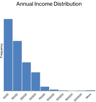
3.2.1.2 Skewness Having data with a very large range of values can impact the results of the analysis. To solve this, the team looked for numeric variables with a large range of values. These features include Income – Annual, Income – Gross, and Percent Pov-erty. The histogram below in Figure 2 shows an example of the skewness present. In this case, the data ranged in value from 0 (a valid value as some patients are homeless and unemployed) to in excess of $250,000,000 per year. Although outlier detection hasn’t yet been performed, it is obvious here additional cleaning steps will have to be taken. A natural log transformation was done on these variables to reduce the skewness and return the values to a more normal distribution.
Figure 2: Raw annual income histogram
3.2.1.2 Outlier DetectionA crucial step in preparing data for machine learning prob-lems is outlier detection. In the context of this problem, outlier detection becomes a necessity after simply inspecting the distribution of the continuous features. For exam-ple, some patients have an annual income exceeding $250 MM. Similarly, other pa-tients claim more than forty dependents. It is beyond the scope of this project to
inves-tigate such extremes, but in the given data set, such observations are outliers. Addition-ally, most features are categorical and verified by the data provider. For example, the data set containing diagnoses are known to be correct. A simple check of categorical features to ensure consistency was completed; none of the categorical features were marked as a concern for outlier detection.
The concern is finding outliers in a multivariate data set rather than plotting each continuous feature. One goal of this exercise is to capture the interactions of the features collected. Additionally, a multivariate outlier detection method provides greater effi-ciency. Outlier detection is valuable because for the algorithms benchmarked, outliers will impact each one to varying degrees of severity.
To address the multivariate outlier detection problem, the Isolation Forest algorithm was used to identify possible outliers. Many other outlier detection algorithms, “con-struct a profile of normal instances, then identify anomalies as those that do not conform to the normal profile … this leads to two major drawbacks: (i) these approaches are not optimized to detect anomalies … (ii) many existing methods are constrained to low dimensional data and small data size because of the legacy of their original algorithms” [12].
Isolation Forest, “proposes a different approach that detects anomalies by isolating instances, without relying on any distance or density measures … anomalies are ‘few and different,’ which make them susceptible … to isolation. Because of the suscepti-bility to isolation, anomalies are more likely to be isolated closer to the root of an iTree [ isolation tree]” [12].The Isolation Forest algorithm is an ensemble technique: mean-ing that many isolation trees are used to locate the ‘isolated’ instances.
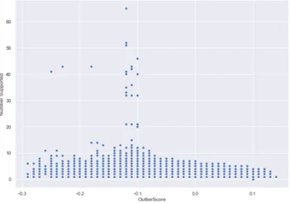
After applying the Isolation Forest algorithm to the data set, certain features such as income and the number of dependents most certainly contain outliers. First, observe
Figure 3 and Figure 4. From this visual, the outlier score (x-axis) is plotted against the feature’s recorded values (y-axis).
Figure 3: Outlier scores: log normal income
Gross income is presented on a logarithmic scale in Figure 3 and the associated iso-lation score is found on the x-axis. The graph shows excessive income is associated with a lower, and therefore, more anomalous score. Likewise, patients who report high dependents are flagged as outliers in Figure 4.
Figure 4: Outlier scores: number of dependents
Now the anomalous observations are visualized, the best plan for proceeding with any potential anomaly is to discuss validity before simply removing. After meeting with subject matter experts associated with the facility, it was determined the observations with very high income and/or dependents are not valid. To overcome this, an upper threshold on income and the number of dependents was applied. The features with threshold applied were left in the data set so they could be evaluated for value to the algorithms to be selected in the screening process.
3.2.2 Feature Engineering Even with the large amount of data extracted from the pa-tient electronic medical records, there are many more features to explore by simply deriving from the raw features. Feature engineering is an often overlooked, yet critical aspect of model building. Additionally, feature engineering can be thought of as the ‘art’ aspect of data science: “As with many questions of statistics, the answer to ‘which feature engineering methods are the best?’ is it depends. Specifically, it depends on the model being used and the true relationship with the outcome” [15]. The approach taken to feature engineering was a deliberately naïve approach: creating and testing features,
then consulting with subject matter experts as a sanity check. This iterative process of feature engineering, testing, and consultation with SMEs gives confidence the final set of features are both statistically and practically relevant and significant.
While the electronic medical records provide a substantial amount of useful data, there are many ways to augment this data via feature engineering. “Feature engineering is the act of extracting features from raw data and transforming them into formats that are suitable for the machine learning model. It is a crucial step in the machine learning pipeline, because the right features can ease the difficulty of modeling, and therefore enable the pipeline to output results of higher quality” [14]. Feature engineering must be done with care as it opens the door for data leakage, which refers to the unintended transfer of information between the training and test data sets. First, several features were created from the provided actual appointment date and the date the appointment was booked. Using provided dates of appointment scheduled date and actual appoint-ment date, the length of time between when the appointappoint-ment was scheduled and when it should occur was calculated. This yielded the number of days elapsed between the dates as a potential feature. The team hypothesized that more urgent appointments will have a shorter lead time, and thus an increased probability of making the scheduled appointment. Conversely, the appointments with a longer lead time are hypothesized to have a higher associated probability of missing the appointment. The date of appoint-ment also allowed for extraction of such potentially useful features as time of the month (beginning or end) and the day of week. The appointment date also allowed inclusion of features which are weather related. For example, the creation of a season variable as a proxy for weather data. The reason for this decision is while actual precipitation data is predictive as determined by an early prototype model, careful consideration of the end usability of the model is important. The vision for the model in production is to refresh the data frequently for retraining. It would be a herculean effort to continually update the patient predictions whenever a weather forecast is published. Additionally, utilizing weather forecasts for future appointments only adds more variability in the model. As such, season is utilized as a proxy for general weather trends.
Another feature derived from the electronic medical records is age at the time of the appointment. Age also allows for further classification into distinct bins to capture gen-erational differences. A patient’s zip code is also considered as a potentially relevant feature. Zip code, city name, and state are all generated features and candidates for model inclusion. It is important to note that while the data came from a center in Okla-homa, there are a few out of state patients from neighboring states. When considering zip codes, the driving distance for each patient to make their appointment was calcu-lated. In an exploratory analysis, the team realized several patients moved during the training and testing time period. To deal with this change over time, the primary key for distance calculations was a unique combination of patient ID and appointment date.
While it is relevant to consider some general aspects about a patient such as driving distance, age, and others, it is potentially significant to consider a patient’s past missed appointments. For example, if a patient has missed many appointments in the past, his or her past behavior could be a potential feature for predicting future behavior. This feature is also an area of caution: incorrectly grouping and sorting patients could result in data leakage. To handle any data snooping issues, a lookback window was derived
for each patient. The lookback window operates such that the last time a patient was seen either results in a penalty of one if he or she missed their appointment or zero if the patient kept their appointment. For each appointment, this lookback window is up-dated. Additionally, a cumulative score of past missed appointments was created. As with age, this permits further classification into low, medium, and high-risk patients. While this feature is one that is both intuitive and supported by current research, it also is an area of caution when considering the care needed when preparing training and testing data sets that do not ‘peek’ into the future. For example, if predicting a month of appointments as a batch, only consideration of the patient’s past behavior at the time of the actual appointment should be added to the model. No future appointments should ever be considered in this feature.
In addition to the features discussed, research and subject matter experts both en-couraged inclusion of indicators for chronic medical conditions. These were derived by matching disease indicators from claims submitted after the visit on the same date as the appointment. Chronic conditions were defined as one or more of a diagnosis of diabetes, hypertension, depression or anxiety. Depending on the date of the claim, if the International Classification of Diseases (ICD) version 9 (ICD9) or version 10 (ICD10) claim code for a chronic conditions was present, they were coded by assigning the feature of the condition name to a binary code of 1 for present or 0 for absent. A feature was added to indicate if two or more of the chronic conditions are present. Med-ically complex patients like these are challenging to manage from the standpoint of the care team and successful treatment of these patients often requires regular appoint-ments. If these patients are more likely to miss appointments, interventions can be fo-cused on them to try to get them in for care. To avoid data leakage, the chronic condition features were updated after every completed visit to reflect the information that would be available at the time the next visit was scheduled. The same sliding window approach was applied to only consider diagnoses at the current time; no future appointment data was used to determine if a patient has a condition. For new patients, these features were set to zero, as documented health conditions are not available at the time of scheduling a new appointment.
The features created, in addition to the raw data found in the electronic medical rec-ords are all candidates for the predictive model. By creating these features, a plethora of potential variables was added to the data. After encoding categorical features, there were nearly 1,000 unique predictors to consider for the model. As indicated, a naïve approach to feature selection was taken considering all features first and then subject matter experts provided sanity checks regarding the features which might be relevant to the issue.
3.2.3 Feature Screening As with feature engineering, it is difficult to overstate the importance of not allowing data leakage in this study. Feature screening allows another opportunity for leakage to occur. An example of this common mistake is when a data set is combined into an aggregate set consisting of all observations in a study. Then, a feature screening algorithm is utilized on the aggregated data set. After features are selected, the smaller subset of critical predictors is split into training and test data sets.
This is a common mistake in data analytics and machine learning problems that intro-duces bias to the modeling process, as features were selected on observations from both training and testing sets.
To overcome any data leakage issues, 2018 appointments were set as the test data. Model performance on this data set indicates the predictive power of the algorithm in the real world and is the best reflection of how this model will behave in production. As a part of the process, the necessary steps to remove all 2018 appointments from the data set used to screen and select predictive features were taken.
The team chose to try two different algorithmic solutions to feature screening, Ran-dom Forest Classifier and XGBoost. Both are common methods of feature screening and since peak performance of the model is of interest here, a comparison and contrast of the results of both algorithms with this data set are examined.
A Random Forest Classifier is a popular tree-based approach for feature screening; the Random Forest algorithm utilizes a multitude of decision trees to reach a solution and helps determine the most significant features via an ensemble technique known as bagging: “Random Forests … decorrelates the [decision] trees. As in bagging, we build a number of decision trees on bootstrapped training samples … each time a split in a tree is considered, a random sample of m predictors is chosen as split candidates from the full set of p predictors. The split is allowed to use only one of those m predictors. A fresh sample of m predictors is taken at each split, and typically the team chose 𝑚≈"𝑝 that is, the number of predictors considered at each split is approximately equal to the square root of the total number of predictors” [16]. When applied as a screening algo-rithm, each features’ index, which can be thought of as relative importance as a predic-tor, is determined by the average decrease in the Gini index, whereas the Gini index is a measure of impurity: smaller values are better than larger values, with zero being perfect. The Gini index for a binary classification problem is seen below. 𝑃%&is the
proportion of data points in region 𝑅_𝜏 in class k, where k =1 [15].
𝑄 , (𝑇) = 1 𝑝%&(1 − 𝑝%&) 4
&56
Strong predictors will decrease the Gini index, “we can add up the total amount that the Gini index is decreased by splits over a given predictor, averaged over all β trees” [16]. In a nutshell, the goal is to find the top predictors in the data set that ultimately predict no-show status; simply use the average decrease in the Gini index to arrive at which features help to accomplish the analysis goals. With a data set of nearly 1,000 features, it is necessary to apply a feature screening algorithm such as a Random Forest Classifier to help identify the critical few features in the study.
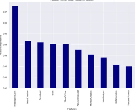
Care must be taken when taking such a naïve approach to remove multicollinearity after an initial screening, as there are redundant features returned, such as gross income, an-nual income, and percent poverty. Gross income and anan-nual income are highly corre-lated (r = .986). Additionally, annual income and percent poverty are also highly cor-related (r = .999). Steps were taken to remove these corcor-related features. These features,
derived via a feature selection algorithm, were reviewed with a subject matter expert associated with the facility. The screening technique identified the features in Figure 5, below, as relevant predictors for no-show status
Figure 5: Random Forest Features
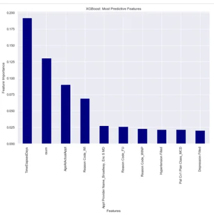
The team also completed feature screening on the training data set by applying XGBoost. The selection of XGBoost as a secondary screening algorithm was made because, while computationally expensive, it gives the team another ensemble tree-based approach to selecting the best features among a possible 1,000 demographic, ge-ospatial, and medical predictors. The team also focused on how XGBoost differs from a Random Forest Classifier as additional justification in applying two different algo-rithms in feature selection. First, consider one of the fundamental differences between
boosting and bagging. Random Forest, based on bagging, constructs the trees in the ensemble in parallel, or independent of other trees. XGBoost, on the other hand, con-structs trees in the ensemble sequentially; each new tree reduces the previous prediction errors. Both methods are ensemble techniques, but differ in the way each ensemble is built. XGBoost, just as Random Forest, allows a determination of feature importance. XGBoost feature importance is determined by each feature’s gain. Gain, in this context, can be thought of as the contribution of a feature, similar to the Random Forest feature screening. With this interpretation in mind, XGBoost was employed, in addition to Random Forest, to determine which features should be used in the final algorithm. The top ten features selected by XGBoost are seen in Figure 6.
Figure 6: XGBoost features
While this list of top features confirms some of the findings the research team antic-ipated, such as the days elapsed between book date and actual appointment date, it is never wise to settle on one subset of predictors based solely on one algorithm.
The top features indicate time variables are top drivers in predicting no-show status. These results are consistent with results found in the literature. From an ethical per-spective, it is observed that race and ethnicity are not considered top drivers in model performance. As the study continues, and more features are added, removing race and ethnicity completely may be the best path forward to minimize racial bias in the model. A significant overlap in the selected features between the two screening algorithms is
seen. As indicated, a naïve approach to the feature selection was taken, implying no features were removed prior to feature screening. To resolve the issue of which subset to use, the team presented the findings to a subject matter expert associated with the facility. The XGBoost features were selected by the subject matter expert based on ex-perience in the field. Because of the significant overlap, the decision to use features selected by XGBoost was not considered detrimental to the development of the algo-rithm.
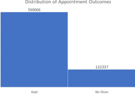
3.2.4 Class Imbalance In the data set, the no-show appointments only represent 13.47% of the response variable, appointment status, as seen in Figure 7, below:
Figure 7: Appointment outcome distribution.
This class imbalance leads to a unique set of challenges in statistical machine learning. With an imbalanced data set, reporting a classification algorithm’s accuracy is decep-tive; simply classifying all labels as ‘Occurred’ (true negative) yields an accuracy better than chance, thus misleading the audience to believe an algorithm is more predictive than the actual performance. In this study, accuracy
((𝑇𝑃 + 𝑇𝑁)/(𝑇𝑃 + 𝐹𝑃 + 𝑇𝑁 + 𝐹𝑁))
(1)
is reported, but success is defined in terms of recall
(𝑇𝑃/(𝑇𝑃 + 𝐹𝑁)).
In the analysis, the imbalanced nature of the data is addressed by implementing the Synthetic Minority Over-sampling Technique (SMOTE) algorithm. By utilizing the SMOTE algorithm, “the minority class is over-sampled by creating synthetic examples rather than by over-sampling with replacement … The minority class is over-sampled by taking each minority class sample and introducing synthetic examples along the line segments joining any/all of the k-nearest neighbors” [19]. The creation of the synthetic data points in the training sample allows the decision boundary of the classification to become much more pronounced for the ‘no-show’ class. The inclusion of the new syn-thetic points allows the classifier to better learn the feature/target mapping: “More gen-eral regions are now learned for the minority class samples rather than those being sub-sumed by the majority class samples around them” [19]. For illustrative purposes on the importance of applying SMOTE, a Random Forest Classifier was used to predict no-show status in the data set because a non-linear, non-parametric ensemble method makes no a priori assumptions about the data set and gives a strong first pass attempt to model the relationship. Once again, the purpose of this method is to illustrate the boost in recall when SMOTE was applied. The Random Forest was trained on 70% of the center’s appointments, with a 30% independent holdout test data set. The test data performance results in a recall of 55%, with an overall accuracy of 67%, as derived from the confusion matrix in Figure 8. The impact of SMOTE cannot be overstated in this model. It is evident that SMOTE allowed the model to determine a more distin-guishable decision boundary for the minority class: no-show appointments. The benefit of using SMOTE on the training data is not trivial when evaluating the test data perfor-mance: recall of the no-show class is 13% when SMOTE is not implemented. However, once SMOTE is used to balance the classes, recall of the no-show class is 56%, as seen in Figure 8.
3.3 Machine Learning Process
After reviewing predictive features with the subject matter experts, the features re-ceived a high acceptance rate. Before beginning the modeling details, it is important to emphasize the model, once in production, is most likely going to make predictions on a regular batch basis. Because of this restriction, there will be multiple test data sets. Test data was segmented into months January through October 2018. While time is an important component in this analysis, the software is not performing a traditional time series ‘forecast’ of missed appointments; the importance of time is most relevant in that predictions are made considering a patients past no-show performance and chronic dis-ease status at the time of making the appointment.
In machine learning, the first step is always to understand what type of problem one is attempting to solve. Working with the clinic and their subject matter experts, a clear, concise objective was developed. The question of interest/objective is to “Attempt to predict no-show medical appointments and provide our staff with information on which patients are at a high risk of no-shows.” The second step is to determine what types of algorithms are appropriate and what volume of data is available to answer the objective. The team examined the available data, as well as the data sources available for use in this research problem. The examination of all available features indicated a clear re-sponse variable: ‘Appt Status Desc.’ This feature is a simple text field indicating whether an appointment occurred or did not occur. Since the data set has a labeled outcome variable, also known as a response variable or dependent variable, the problem is narrowed down to that of a supervised learning problem with a binary outcome. With the second step, determining what type of problem to solve now complete, the next step is to select various classes of algorithms to attempt to solve the question of interest. In a field experiencing the rate of change currently occurring in machine learning, it is difficult to stay abreast of all the rapid advancements in research, optimization, open-source libraries, and algorithms. The team is simply applying the best reopen-sources to solve the question of interest: predicting no-show appointments with the best accuracy and recall possible and outlining steps to operationalize this classification model.
The approach taken in this analysis is through the lens of statistical machine learning. While the goal is to provide the primary care facility with the best actionable insight possible, due diligence must be taken to evaluate a myriad of classifiers. The perfor-mance of each will be addressed. The approach taken was to build linear classifiers and incrementally add complexity with nonlinear models in a progressive manner. This ap-proach was taken so to allow for careful consideration of each model in isolation, the associated pros and cos, and limitations before advancing to newer approaches. How-ever, during the research of this analysis, new and useful algorithms were discovered. The full list of classification methods considered spans classical and recent develop-ments in machine learning: Logistic Regression, Naïve Bayes, Stochastic Gradient De-scent, Decision Tree Classifier, Extra Trees Classifier (Extremely Randomized Trees), Random Forest Classifier, Adaptive Boosting (AdaBoost), Support Vector Machine, and Extreme Gradient Boosting (XGBoost). Since the team had many excellent classi-fiers available to select from, a survival of the fittest approach was taken; each algo-rithm followed the same training and testing regime. The top contenders after initial
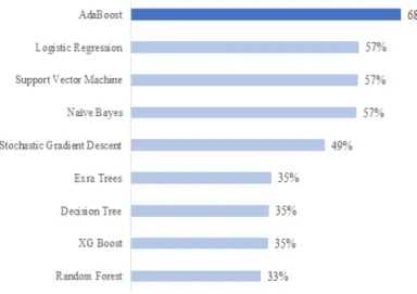
screening of algorithm performance were given further scrutiny and tuning. The algo-rithm average recall scores can be seen in Figure 9, below. The most expensive mistake to make in this domain is a false negative. If the model predicts the patient will attend the scheduled appointment, and he/she does not, there are significant financial and op-erational impacts. It is essential that false negatives also be kept at a minimum, as the intention is to put this model into production. A model that effectively balances false positives and false negatives will result in a new operating regime for the facility as there will be a noticeable step change in the percent of no-show appointments.
Figure 9: Average recall score
It is observed that Adaptive Boosting has the clear advantage among all algorithms considered. It’s not surprising to see a boosting algorithm leading more traditional ap-proaches. It is worthwhile to explain boosting, its mechanics, and associated benefits. Since the highest scoring model on the test data set was AdaBoost, a brief explanation of the theory of boosting is in order.
3.3.1 Boosting Boosting is a sequential process that combines multiple weak classifiers that ultimately yield a model committee that performs much better than any individual weak model. Each weak classifier is combined into an ensemble. Boosting performs in such a way that “base classifiers are trained in sequence, and each base classifier is trained using a weighted form of the data set in which the weighting coefficient associ-ated with each data point depends on the performance of the previous classifiers. In particular, points that are misclassified by one of the base classifiers are given greater weight when used to train the next classifier in the sequence” [18]. The greatest ad-vantage to boosting is the weighting of the classifiers. This iterative process allows improvements when a classification task is not straightforward, as most problems are
not in business settings. In boosting, the incorrect predictions alter the weighting coef-ficient as the training process progresses, “At each stage of the algorithm, AdaBoost trains a new classifier using a dataset in which the weighting coefficients are adjusted according to the performance of the previously trained classifier so as to give greater weight to the misclassified data points” [18]. An illustrative example of how boosting works in the training process can be seen in figure 10.
Figure 10. Boosting process for training data – adapted from Bishop, et. Al [18]
In Figure 10, the blue arrows represent a portion of the training data. The weak clas-sifiers are denoted by 𝑌𝑚(𝑥) and weights are represented by 𝑤𝑛(𝑚)
.
Recall from theprevious definition that this subset is weighted, depending on the previous classifiers performance. The green lines indicate the sequential nature of training in Adaptive Boosting. The resulting algorithm, YM(x), is an ensemble of the individual weak
clas-sifiers. The individual models are combined in the final classification model.
It is clear how boosting is a benefit to this problem. As one can imagine, modeling human behavior may not be optimally achieved on a simple, single decision tree. Some features in the model are clear and distinct, and on their own, may provide healthcare providers a good heuristic for when a patient will not show for an appointment, such as days elapsed between booking date and actual appointment date. However, as consid-eration is given to other less obvious predictors such as income level and geospatial attributes, the prediction task becomes more complicated, as the features in concert re-quire the pattern recognition obtained via machine learning.
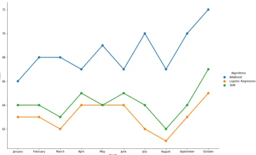
3.3.2 Boosting Results With the most successful model identified as AdaBoost and visualized in Figure 11, a focus on the specific results of AdaBoost are in order.
Figure 11: Recall comparison on test data of top 3 algorithms 3.4 Model Explanation
3.4.1 General Model Interpretation One of the most challenging aspects of presenting machine learning models to a customer is the ability to clearly interpret a complex model. The winning solution, based on boosting, is a clear example. The proposed so-lution to this problem is an ensemble. Ensemble models, while effective, can be difficult to interpret. There exists a trade-off between interpretability and model performance. In the study, it was observed that Logistic Regression, a linear model, offers decent results. This model could be easily explained to the customer. However, consider the lift in recall achieved through Adaptive Boosting. This increase in recall translates to a significant savings for the customer. Because the winning solution is a tree-based model, it is not difficult to determine feature importance as discussed in the feature engineering section. The difficulty lies in helping the customer understand what is go-ing on ‘under the hood.’ More specifically, in the case of the solution, the team sought to find patients that increase the probability of a no-show and attempt to isolate the model effects.
To aid in understanding how the model functions, the team presents an interpretation of the top features using SHAP (SHapley Additive exPlanations). “SHAP assigns each feature an importance value for a particular prediction. Its novel components included: (1) the identification of a new class of additive feature importance measures, and (2) theoretical results showing there is a unique solution in this class with a set of desirable properties” [25]. SHAP provides a model-agnostic approach to interpretation: ensemble methods and deep learning models alike become less of a black-box approach.
The concept of SHAP is that the model under evaluation is trained on all possible feature subsets. During this process, Shapley values derive an importance metric for
each feature that influences the model prediction. This metric is calculated by training two separate models: one contains the feature in question, the other excludes the fea-ture.
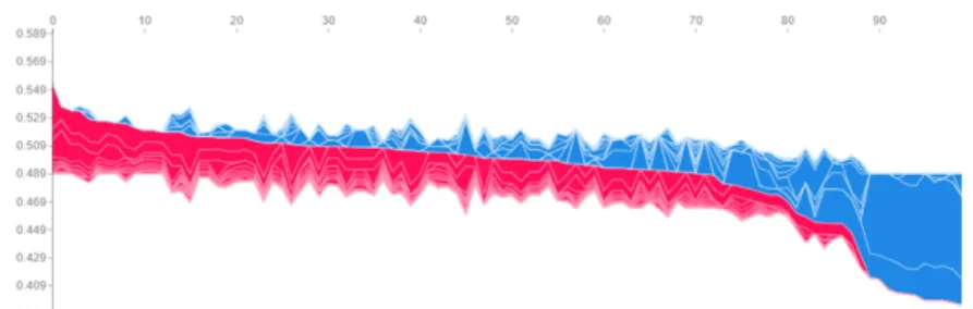
Using a sample of 100 patients from October 2018, a decision was made to imple-ment Shapley values for model interpretation, as well as some insight on when the fa-cility may want to intervene. Red is associated with increased probability of missing an appointment, while blue is associated with decreased probability of missing an appoint-ment. The values are visualized in Figure 12.
The figure below shows a clustering of patients and their associated probability of missing an appointment in October 2018 where the y-axis represents the probability of missing an appointment and the x-axis represents each patient in the sample. The most at-risk patients can be thought of as those associated with the leftmost cluster of model predictions in red. This type of clustering would be useful in scheduling and actively double booking appointment time slots. However, the goal is to isolate the most im-portant features. By doing so, the facility could identify thresholds of predictor values that could be used to increase communication to at-risk patients.
Figure 12: Sample cluster of patients’ no-show probability
The top three features found in the ensemble are:
i. Time elapsed between booking date and appointment date (TimeElapsedDays) ii. Cumulative sum of past missed appointments (csum)
iii. Age of patient (AgeAtActualAppt)
It is hypothesized that elapsed days is a predictor of patient behavior as it relates to show status. There are many possible reasons for patients which can affect a no-show: priorities change, significant life events occur, and people become forgetful. While at the level of the individual patient, no insight is available, some trends over the
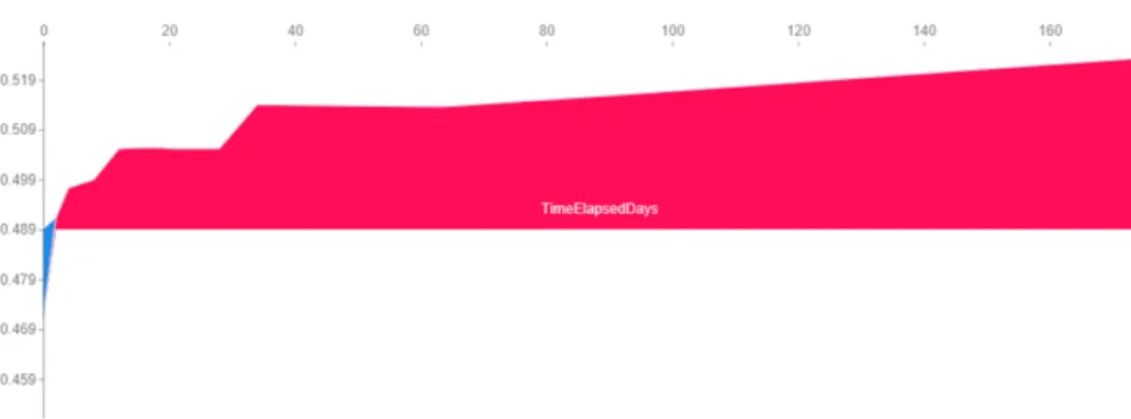
population can be determined as reflected in the sample below. By examining the effect of this feature on the model’s predictions, an expected trend in Figure 13 is seen.
Figure 13: Impact of elapsed time on probability of no-show
The research team interprets the effect of this feature as greater time elapsed between booking the appointment and the actual appointment is associated with a higher proba-bility of missing the appointment. Further insight can be drawn: notice the step changes present. There are slight elevated probabilities for appointments booked fifteen to twenty days in advance. However, the largest step change is seen when the appointment is booked approximately thirty days in advance. This probability continues to increase after a sixty-day interval between book date and appointment date. It may be ideal for patients who book appointments approximately one month in advance to receive addi-tional communication reminding the patient of the appointment. Appointments booked
six months in advance may also require more attention.
Figure 14: Impact of previous missed appointments on probability of no-show
The patient’s missed appointment history was found to be the second most influen-tial feature in the model. However, it is unclear from the model exactly when a patient’s past missed appointments changed their classification to a mild no-show risk to that of elevated risk.
The cumulative score, calculated by means of a lookback window, is an intuitive predictor. If a patient missed many appointments before, he or she may continue this behavior for future appointments. The Shapley values help visualize that missing at least two appointments is the beginning of an elevated probability of missing an ap-pointment. This relationship is seen in Figure 14. A step change is noticeable from the fifth missed appointment to the sixth. Likewise, there is a significant step change from the eighth missed appointments to the ninth. Finally, once a patient misses eighteen or more appointments, the probability continues to increase. These critical changepoints
will be crucial for healthcare facilities to manage. It is not implied that these change points are permanent; retraining the model and monitoring accuracy are assumed steps to be known at this point. However, these change points can be taken as heuristics for providers.
Figure 15: Impact of patient age on probability of no-show
The third most influential feature in the model is age. The Shapley values are seen in Figure 15. It was hypothesized that older patients have less of appetite for missed appointments due to the inherent risk of aging and failing health. From the Shapley values, it can be seen younger patients are associated with a higher probability of miss-ing an appointment. However, after approximately age 55, the probability of missmiss-ing an appointment decreases significantly.
One final look at the sample is presented in Figure 16. This time, a simple plot of the 100 patients as they are presented to the model is seen. This test period demonstrated superb results: recall was 72% and the AUC was .70. Further mining and pattern recog-nition is recommended for the facility to reap the full benefit of this model; this type of visualization is useful for finding more clusters of at-risk patients and strategy devel-opment for preventing more no-shows.
Figure 16: Probability of no-show by patient
3.4.2 Unique Patient Explanation Now the impact of the top predictive features is better understood, further establishment of trust in the algorithm using Local Interpret-able Model-agnostic Explanation (LIME) can be created. LIME allows for demonstra-tion of the model on individual predicdemonstra-tions; anyone can see the predicted probabilities and the impact all features have on the model. LIME allows for a patient-by-patient basis to understand the predictions. Ultimately, Shapley values and LIME can be used in conjunction to better understand the output of any machine learning model. LIME excels as an exploratory data analysis tool that gives intuitive explanations for model predictions at a local level, rather than global. LIME enables the team to gain the trust of the end-users, “Understanding the reasons behind predictions is, however, quite im-portant in assessing trust, which is fundamental if one plans to take action based on a prediction, or when choosing whether to deploy a new model” [20].
One of the key differentiators of LIME is the predictions are made locally, rather than globally. This can be confusing to end-users who may not have much experience with machine learning models. As such, the concept of local predictions warrants fur-ther discussion. “Although it is often impossible for an explanation to be completely faithful unless it is the complete description of the model itself, for an explanation to be meaningful it must at least be locally faithful, i.e. it must correspond to how the model behaves in the vicinity of the instance being predicted … local fidelity does not imply global fidelity: features that are globally important may not be important in the local context, and vice versa” [20]. As an illustrative example of the local predictions, consider the graphic in Figure 17.
The model example in Figure 17 has a clearly nonlinear decision boundary much like the general model explanation. The bold red cross is the subject of predictive in-terest. “LIME samples instances, gets predictions using f, and weighs them by the prox-imity to the instance being explained (represented here by size). The dashed line is the learned explanation that is locally (but not globally) faithful” [20]. Equipped with this
Figure 17: Decision boundary visualized
understanding of LIME, a few examples of explaining the boosting algorithm are in order. The dataset utilized is from a sample of patients in October 2018.
Patient 270 in this sample is chosen for the demonstration of LIME. Some quick facts about this patient reveal that this individual has a history of making appointments, had little time between booking the appointment and the actual appointment, and was 84 years old at the time of booking.
LIME gives the prediction probabilities in Figure 18.
Figure 18: LIME predictions for patient 270
LIME gives, for all features in the model, a simple association: either a feature is associated with no-show or is associated with making an appointment. From this out-put, it can be concluded this patient was predicted as “show” because: low number of missed historical appointments, not in 20-33 age bin, negligible days between booking date and appointment, no dependents, and travel distance to facility. Meanwhile, other factors at play increased the no-show probability such as reason for appointment, health conditions, and a high poverty percent in the county of residence. The model predicted this patient would ‘show’ for this appointment, or a label zero. The actual result was the patient made the scheduled appointment; this prediction is a true negative.
To further demonstrate the power or LIME, another patient is considered. The pa-tient being evaluated is again sampled from the October 2018 appointments (papa-tient #95). LIME gives a no-show probability greater than 50%. This patient was predicted to no-show; the actual outcome was the patient did not show. Using the output from LIME, the team developed the following display to aid end-users understand feature impact for this at-risk patient in Figure 19:
Figure 19: Patient 95 classification factors
Model explanation tools like LIME and SHAP give confidence to users to act upon this model. While ten months of superb results in terms of accuracy and recall were seen, SHAP and LIME help researchers and users untangle the model and understand why the results in Figure 19 were obtained. Aside from an academic exercise, LIME and SHAP help explain the model’s predictions to end users: an essential step in estab-lishing trust in the model’s predictive output.
4
Traditional Statistical Approaches
As indicated, the current research in predicting no-show appointments mostly uti-lizes linear models. Per research and a literature review, the first attempt to model no-show appointments was by Dove and Schneider in 1981 [22]. The study utilized ordi-nary least squares to predict a given days’ number of no-show appointments. The results of the study were statistically significant, inspiring other such studies and inspiring a new statistical process control mindset to healthcare operations. In 2014, Erdem et al. conducted a similar study. The biggest difference was the problem was transformed from a regression problem to that of classification. This study also resulted in statisti-cally significant findings [23]. Erdem et al. achieved an area under the curve (AUC) between 0.64 and 0.70 in multiple iterations of their model [23]. Later, in 2017, Goffman et al. attempted a larger scale study of predicting no-show appointments. The methodology utilized was similar, but more effort was placed on feature engineering.
The results were a significant improvement. This study predicted across multiple facil-ities and resulted in an AUC ranging between 0.71 and 0.763 across the various facili-ties in the study [24].
5
Model Deployment
The FQHC fully intends to use this machine learning model in production to reduce the count of no-show appointments and thus, reduce operating costs and waste. While the model predicts reasonably well, upkeep is necessary. At a minimum, the team pro-poses retraining this model monthly. Furthermore, it is also to update information about each patient before the model is retrained. For example, if a patient had missed three appointments in January 2018, it is essential to update that patient’s history of missed appointments, as a higher probability of missing an individual appointment is likely when one has missed appointments in the past. Other considerations should be made and updated as the model is in production such as changes in zip code, income changes, and the number of dependents. A reasonable recommendation for keeping an updated database is to ask all patients to update these important features annually. Another area of consideration is how to handle new patients. For these instances, it is proposed that all new patients be assigned a low risk profile, or zero missed appointments, until be-havior dictates otherwise.
Perhaps the most difficult question from an implementation standpoint is how to intervene when a patient is predicted to miss an appointment. While this decision is ultimately up to the facility, a tiered system based on the probability predicted is pro-posed. For those predicted to not make their appointment, the probability associated with that prediction must be considered before acting. One suggestion is to simply dou-ble book those with a high probability of not making the appointment. For those who are slightly over the prediction threshold, it is recommended that the facility attempt to contact the patient. For example, a phone call, text, or email would likely suffice to remind patients of upcoming appointments. This two-pronged approach merely pro-poses some suggestions for action that will be the responsibility of the facility. The Goffman study [24] is notable here as a possible source of potential interventions, as they did a rigorous comparative study of different interventions and their efficacy.
6
Results
6.1 Comparison of Results
Adaptive Boosting outperforms the other algorithms in the study in terms of recall and accuracy. However, while robust, Adaptive Boosting is not without competition. It was seen previously that Support Vector Machine and Logistic Regression also offer compelling results. To make the final determination, McNemar’s test for statistical sig-nificance is used. The results are presented in Table 1. McNemar’s test for sigsig-nificance is appropriate on classification models when the number of instances each classifier got
correct and incorrect is known. McNemar’s test for significance compares each algo-rithm in a pairwise fashion; a conclusion on distinct pairs significance of results is re-viewed. Additionally, McNemar’s test is a nonparametric test, meaning there are no strict distribution assumptions to meet.
The test statistic is calculated as: [25]
𝜒 = (𝑏 − 𝑐)
B
𝑏 + 𝑐
Table 1: Generic confusion matrix values for McNemar’s Test
Test 2 Positive Test 2 Negative Row Total Test 1 Positive a b a + b Test 1 Negative c d c + d Column Total a + c b + d n The null and alternative hypotheses are
𝐻D:𝑝F = 𝑝G
𝐻6: 𝑃F≠𝑃G
If it can be found that p > alpha, then the conclusion is to fail to reject the 𝐻D. This
would indicate there is no difference in the classifiers’ errors. However, if p < alpha, reject 𝐻D. This indicates there is significant difference in the classifiers’ errors. For
this experiment, a significance level of 0.05 was used. The results of the Adaptive Boosting McNemar test are presented in Table 2:
Table 2: McNemar’s Test Results
Comparison Result
Ada Boost vs. Logistic Regression Significant at level 0.95 Ada Boost vs. Naïve Bayes Significant at level 0.95 Ada Boost vs. Support Vector Machine Significant at level 0.95 Ada Boost vs. Stochastic Gradient Descent Significant at level 0.95 Ada Boost vs. Decision Tree Significant at level 0.95 Ada Boost vs. Extra Trees Significant at level 0.95 Ada Boost vs. Random Forest Significant at level 0.95 Ada Boost vs. XG Boost Significant at level 0.95
The McNemar test indicates if there is a significant difference in the count of errors. The research team observe statistical significance in the test results: it was determined to reject 𝐻D in each pairwise comparison of the leading algorithm, Adaptive Boosting.
The conclusion is each pairwise comparison of algorithms has a different proportion of errors on the test period of January 2018 to October 2018. The other two leading algo-rithms, Logistic Regression and Support Vector Machine, show significance on most pairwise comparisons. However, one differentiating factor is that only Adaptive Boost-ing shows significance on all pairwise comparisons.
After concluding AdaBoost the best algorithm for this prediction task, analysis of algorithm performance throughout each month of test data was performed.
Addition-ally, a second round of testing with a slightly lowered probability threshold was con-ducted. This approach allows a presentation of both a conservative approach to identi-fying no-show patients and an aggressive approach. More true positives are gained by lowering the probability threshold, but this approach also incurs more false positives. If the customer simply wishes to communicate via text message or email for appoint-ment reminders to those likely to miss an appointappoint-ment, the aggressive prediction thresh-old may be an acceptable approach. However, if the site wishes to employ the algorithm for purposes of double-booking, the conservative approach is likely more appropriate. Figure 20 illustrates the recall for the two methods on each month of the test period for the top three performing algorithms.
Figure 20: AdaBoost vs logistic regression recall scores in 2018
With both methods, some seasonality in the results is observed. For example, notice the cyclicality present in the summer months. The benefit of the sliding window ap-proach is apparent in Figure 20. By considering changes in age, zip code, diagnoses, and behavior, the team was able to obtain better recall results month over month, while maintaining an average accuracy of approximately 68%.
Another challenge in this prediction task is the fact of modeling human behavior. One way the team helped guard against model performance degradation is to include whether a patient is being seen for the first time or not. While this feature plays a role in maintaining good accuracy and recall, the algorithm exhibits slight degradation as the percent of new patients increase. It is also hypothesized that summer vacation and holidays during this period could be responsible for the cyclicality. Further work on the algorithm will derive additional features to address this observed seasonality.
7
Conclusions
Determining the probability of a patient ‘no-showing’ an appointment can yield sig-nificant financial and operational improvements for health care providers. For patients, practices who actively identify and intervene with patients to reduce no shows help patients overcome barriers to care and to have better health outcomes. The research team demonstrated a process to intake clinical, demographic, financial, and other types of data and successfully used a modern machine learning algorithm to predict the prob-ability of no-show appointments. Using a survival of the fittest approach to nine differ-ent algorithms, including a classical statistical model and newer machine learning tech-niques, yielded a clear winner, AdaBoost. AdaBoost outperformed all the other algo-rithms in a statistically meaningful manner. A direct comparison of AdaBoost and Lo-gistic Regression shows AdaBoost to be more effective at predictions on this data set. This is the first time the team is aware of a direct comparison between Logistic Regres-sion, commonly used in the previous literature on this topic, and a variety of machine learning algorithms has been conducted. Interestingly, Logistic Regression outper-formed five of the new machine learning models and was in a three-way tie for second place using metrics for recall and accuracy. Properly constructed machine learning models can outperform traditional statistical methods, but caution is required to ensure Occam’s Razor is respected by baselining performance with a classical, simple, easy to understand model first. Once a baseline for performance is obtained, then properly de-signed tests and comparisons of results can be implemented to determine if additional performance can be gained.
Implementation of the model would be straightforward once the data is properly cleaned and formatted. AdaBoost doesn’t have large computing overhead and is per-formant enough for this use case without any additional customization or tuning. With the ability of the model to provide information back to the clinic in a meaningful way, the expectation is the implementation will reflect the results observed in the test data. It is the intent of the authors and the clinic to implement this model into production as a pilot project. If the results of the pilot are successful, then a full roll-out to the entire organization would follow. In addition to providing the risk scores and classifications, the research team will work with the clinic to design studies to determine the effective-ness of a number of interventions to additionally reduce no-shows.
References
1. Kheirkhah, Parviz et al. “Prevalence, Predictors and Economic Consequences of No-Shows.” BMC Health Services Research 16 (2016): 13. PMC. Web. 15 Sept. 2018.
2. Lacy, Naomi L. et al. “Why We Don’t Come: Patient Perceptions on No-Shows.”
Annals of Family Medicine 2.6 (2004): 541–545. PMC. Web. 15 Sept. 2018. 3. Anderson, R. T., Camacho, F. T., & Balkrishnan, R. (2007). Willing to Wait?: