Process Flexibility: Design, Evaluation and Applications

Process Flexibility: Design, Evaluation and Applications

Mable Chou∗ _{Chung-Piaw Teo} † _{Huan Zheng}‡

This version: August 2008

Abstract

One of the most effective ways to minimize supply/demand mismatch cost, with little increase in operational cost, is to deploy valuable resources in a flexible and timely manner to meet the realized demand. This notion of flexible processes has significantly changed the operations in many manufacturing and service companies. For example, flexible production system is now commonly used by automobile manufacturers, and work force cross-training system is by now a common practice in many service industries. However, there is a trade-off between the level of flexibility available in the system and the associated complexity and operational cost. The challenge is to have the “right” level of flexibility to capture the bulk of the benefits from a full flexibility system, while controlling for the increase in implementation cost.

This paper reviews the latest development on the subject of process flexibility in the past decade. In particular, we focus on the phenomenon, often observed in practice, that a slight increase in process flexibility can reap a significant amount of improvement in system performance. This review explores the issues in three perspectives: design, evaluation and applications. We also discuss how the process flexibility concept has been deployed in several manufacturing and service systems.

∗

Department of Decision Sciences, NUS Business School, National University of Singapore

†

Department of Decision Sciences, NUS Business School, National University of Singapore

‡

Management Science Department, Antai College of Economics and Management, Shanghai Jiao Tong Uni-versity.

1

Introduction

Selling fruit juices in the canteen of the NUS Business School is a daunting task. The demands for the different types of fruit juice are highly unpredictable, depending on the weather and also the academic calendar of the student population. The problem is exasperated by the fact that the supplies (i.e. fresh fruits) are perishable, and any leftovers often have to be discarded at the end of the day. The stall owner, however, has created an ingenious product to mitigate this problem. This product, called “surprise”, is a random mixture of fruit juices, concocted by the owner, and tailored to the tastes and likings of the student population. You never know what you will get when you order a “surprise” from the fruit stall, but alas, this element of surprise has turned the product into a best-seller, and it is currently the most popular drink in the stall. The implication for operational efficiency is also clear - the stall owner can now cleverly re-shape the demand for the different fruits, and can deploy the available resources on hand to meet the unpredictable demand in a more efficient manner. This is a clear win-win design, both from a marketing and operational perspective.

Demand shaping, however, may not be feasible in all industries. In the event that customer has specific requirements and will not switch to substitute products, some companies have resorted to the use of a flexible product which can be customized to specific use by the customers. Figure 1 shows two examples of flexible product - the first example shows a table that can be customized to varying heights, depending on the needs of the users. The second example shows the design of a flexible book shelf, where the height of the shelving can be customized by the users depending on their needs. Note that additional features have to be built into the product itself to allow for flexible deployment.

The main disadvantage of a flexible product is the associated increase in production cost. To cope with the uncertain demand, the next best thing one can hope for is to exploit commonality in parts and service requirements to make effective use of the available resources. To facilitate rapid conversion of flexible resources and supplies to meet demands for end products, it is necessary for the company to put a flexible product/service delivery system in place to tap into the power of a flexible system. This is the approach adopted by several companies in dealing with their packaging problems. For example, several companies based in Singapore have opted to use flexible packages to economize on the shipping cost and the need to reduce wastage in packaging. In the past, these companies used standard boxes to ship out their customers’

Figure 1: Examples of flexible product.

orders. However, the boxes were often less than half filled, even though the shipping charges were computed based on the volumetric weight1 of the standard boxes used. To save on the logistics cost, these companies have pioneered the use of flexible boxes - where the shape can be customized based on the items packed into the boxes. Figure 2 shows an example of a flexible box used by a Singapore company.

Figure 2: Example of a flexible package. This box can be customized to 4 different heights, by cutting along the edges, up til the grooves as shown on the side of the box.

This strategy has also been adopted by transport authority in several countries to deal with

congestion problem. In the early 70s, the New Jersey Port Authority allowed the morning eastbound traffic to use a lane on the westbound direction of the Lincoln Tunnel, allowing each commuter in the eastbound traffic to save up to 20 minutes every weekday morning. This little added flexibility in the lane direction allowed the transport authority to reap an annual savings of close to 4 million, based on an estimate of productivity value of $2.82 per hour per worker. (Olcott, O. (1973)). This concept is still in use today in many cities, but often with the lane direction reversal controlled by movable barrier systems in order to prevent head on collisions.

Figure 3: Eastbound buses operating on a westbound lane in the morning peak hour in Lincoln Tunnel, New Jersey, in the early 70s. Source: Olcott, O. (1973)

The phrase “process flexibility” can be broadly defined as “the ease of changing the systems requirements with a relatively small increase in complexity (and rework).” This is part of the broader concept of flexibility in service and manufacturing, a rapidly developing area in the academic and practitioner community over the last few decades. We refer the readers to the comprehensive article by Buzacott and Mandelbaum (2008) for an historical overview of the area, and the accompanying insights and future challenges. They presented three different ways of thinking about flexibility: Prior flexibility, State flexibility, andAction flexibility. Prior flexibilityrelates to the design of flexibility into the system by “increasing the variety of initial actions or decisions we can make,” and state flexibility relates to the design of flexibility into the system by increasing the ability to “cope with uncontrollable changes and uncertainty in the environment by trying to be good under any environmental outcome.” Last but not least,

action flexibilityrelates to the ability to respond to “changes and uncertainty that are revealed over time by taking effective recourse action.” Viewed in this framework, process flexibility concerns the incorporation of the right level of state flexibility into the system, by accounting for the level of action flexibility and its impact on cost and performance of the manufacturing and service system.

Process flexibility, as a key concept to quickly respond to demand/supply uncertainties with little cost, has already changed the operational processes in several manufacturing and service industries. The automobile industry, for instance, has moved away from using focused plants (where one plant produces essentially one product) to using modern flexible plants (where one plant produces several products). The Ford Motor Company, for instance, invested $485 million in two Canadian engine plants to renovate and retool them with a flexible system. It has also launched a plan to equip most of its 30-odd engine and transmission plants all over the world with flexible systems.

“...‘The initial investment is slightly higher, but long-term costs are lower in multiplies,’said Chris Bolen, manager of Ford’s Windsor engine plant, which uses the flexible system to machine new three-valve-per-cylinder heads for Ford’s 5.4-liter V8 engine... Ford says the system will help it meet changes in demand. ‘If our business was hit by a significant down sizing from V8s to V6s or V6s to (four-cylinder engines) or diesels in North America, we’ll be able to react to that without years of turnaround,’ said Kevin Bennett, Ford director of power train manufacturing. ’It’s essential we be able to react to the market more rapidly than in the past.’... ”

— Mark Phelan, “Ford Speeds Changeovers in Engine Production”

Knight Ridder Tribune Business News. Washington: Nov 6, 2002.

A survey of North-American automobile industry conducted in 2004 shows that the plants of major automobile manufacturers, such as Ford and General Motor, are more flexible than those 20 years ago (Van Biesebroeck (2004); see also Boudette (2006)). The survey shows that these flexible plants can produce much more types of cars to meet the rapidly changing customer demands while their capacities do not change very much. Suh et al. (2004) contains a case study on how flexibility can be built into the automobile business. The proposal is to have dimensional flexibility in the floor plan of the underbody of the vehicle platform. This can be achieved in various ways (trimming the floor plan for long wheelbase vehicles to meet

the requirement for short wheelbase vehicles, or to weld an extension piece to the floor plan for short wheelbase vehicles to accommodate the long wheelbase vehicles).

The ability to respond quickly to changes in the environment is also important in troops deployment in the military. In military tactics, the reserve force which the commander directly controls is akin to a flexible server: it has no specific task initially in the battle plan, but can be deployed in the most effective way, depending on how the battle evolves on the ground. Of course, the effectiveness of the reserve force depends on the level of state and action flexibility it can be deployed in the battlefield. Unfortunately, the flexible force deployment plan comes with more battle preparation and movement co-ordination on the ground. The daunting task of the commander is thus to come out with a battle plan which can be executed on the ground, and flexible enough to adapt to changes in the environment. The ancient Chinese had apparently mastered the art of flexibility in troops deployment. Folklore has it that the ancient “eight elements battle formation”, a battle array formed by eight fighting units, has the ability to change formation so quickly, for example, from attack to defense formation with fighting units enforcing each other that the enemy “could not see the beginning from the end of the formation.” For ease of command and control, there could only be limited ways to re-deploy the fighting units. However, by co-ordinating their actions together, the formation is able to anticipate and react to a wide range of possible enemy’s maneuver. Finding the structure and logic behind the flexible deployment tactics, and thus uncovering the secrets of this ancient innovation, will be an interesting challenge for the research community. Figure 4 depicts an artist impression of the battle formation used in ancient warfare.

We supplement the review by Buzacott and Mandelbaum (2008) by narrowing our discussion to the subject of process flexibility. In Section 2, we present a basic model for the process flexibility problem, and discuss recent results obtained on the model for a variety of performance measurements (average case, worst case etc.). We review in Section 3 the techniques that can be used to design a sparse and yet efficient process structure, and discuss in Section 4 indices created to measure and evaluate the performance of such a structure. We conclude the paper with a list of recent applications exhibiting a similar theme -that a limited amount of flexibility, properly incorporated into the system, can reap significant benefits. We do not, however, touch on the related issue of how the capacities in the system could be configured. For this, we refer the readers to the works in Van Mieghem (1998), Bish and Wang (2004) and Bish et al. (2005).

Figure 4: A depiction of battle formation in ancient Chinese history

For earlier surveys on related work on manufacturing flexibility, see Sethi and Sethi (1990) and Shi and Daniels (2003). While we try to be comprehensive in our review, it is inevitable that we may be unaware of other important contributions. The fault is entirely ours. Our goal in this paper is to present an overview of some of the recent theoretical results obtained for this class of problems, scattered over a series of papers. However, we have also included some new results and applications that have not appeared elsewhere. For example, the expansion index, obtained from the insight that graph connectivity is a good surrogate for the concept of process flexibility, is described and presented in this survey for the first time. Furthermore, we applied the theoretical results developed in earlier papers to study multi-stage supply chain and troops deployment problems, and obtain several new insights and numerical results for these problems.

2

Models for Process Flexibility

We use a bipartite graph to represent the flexibility structure. On the left is a setAofnproduct nodes while on the right is a set B ofm facility/plant nodes. A link connecting product node

i to facility nodej means that facility j is endowed with the capability to produce product i. Let G ⊆ A×B denote the set of all such links; that is, the edge set of the bipartite graph. Hence, each flexibility configuration can be uniquely represented by a bipartite graphG.

the level of action flexibility, the process flexibility problem boils down to solving the following classical transportation problem onm supply andndemand nodes, with process structure G:

Z_G∗(D) = max n X i=1 m X j=1 xij s.t. m X j=1 xij≤Di ∀i= 1,2, . . . n; (1) n X i=1 xij≤Cj ∀j= 1,2, . . . m; (2) xij≥0 ∀i= 1, . . . , n, j = 1, . . . , m, (3) xij= 0 ∀ (i, j) ∈ G/ . (4)

The vector D = (D1, . . . , Dn) encodes the demand for each product, and Cj represents the capacity/supply at plant j. Our goal is to utilize the capacities at the most efficient manner to meet the demands, subject to the constraints imposed by the process flexibility structureG. While we have presented the action flexibility problem as a static max flow problem, we need to caution that the problem encountered on the ground could be more complicated than depicted by this simple model. The information on D may not be revealed at the same time, and yet the deployment decisions may have to be made on the spot with incomplete information. The objective function may have to take into account the cost impact of overages and shortages, and not mere flow maximization. The actual optimization problem encountered at the operational level is more aptly represented by a multi-stage stochastic programming model, but we have refrained from going into the details here in this paper for ease of exposition.

At the tactical level of state flexibility, we need to design the process structure G, so that the system is able to respond to changes in endogenous uncertainty in the system. i.e., we want the expected maximum flow

ED

Z_G∗(D)

to be as large as possible. The process flexibility problem considered in this paper can be succintly written as the following optimization problem:

max G⊂A×BED Z_G∗(D) .

Note that in essence, the process flexibility structure determines how the system can ef-fectively allocate its capacity to handle the random demand. An alternate measurement to

characterize the performance of the process structure, in the absence of a probability measure on the space of possible scenarios, is via a worst case approach. i.e., we want

min

D∈D

Z_G∗(D)

to be as big as possible, so that the structure G will perform relatively well even in the worst scenario in the set D. This changes the process flexibility problem to the following robust optimization problem: max G⊂A×B min D∈D Z_G∗(D) .

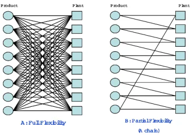
For both objectives, clearly the optimal structure will be the one with full flexibility, i.e., the complete bipartite graph on A and B, containing all the links. However, this level of performance comes at the expense of drastically increase operational and/or communication costs at the operational level. For the process structure to be useful in practice, the number of edges in the graph G should be as small as possible. The central theme of this paper is to use a series of examples and discussions to demonstrate that in most settings, a structure with far fewer number of edges may already perform as good as the fully flexible system. Such results and insights are obviously important and useful in practice.

Studies on process flexibility can be traced back to 1980’s, stemming from the hot topic “Flexible Manufacturing System” (cf. Stecke (1983), Browne et al. (1984)). The focus of FMS is on the trade-off of investment in dedicated versus flexible capacities (cf. Fine and Freund (1990), Van Mieghem (1998)). The challenge there is to understand the economic value of flexible resources in the system, vis-`a-vis its ability to reduce capacity investments. The observation that a partial flexibility structure can perform nearly as well as a full flexibility structure is pointed out explicitly by the seminal work of Jordan and Graves (1995). Their findings were based on a study of GM production network. They calibrated the performance of sparse partial flexibility structures with the full flexibility structure in an extensive simulation. Surprisingly the results showed that a partial flexibility structure, if well designed, could capture

almost all the benefits in the full flexibility structure. They further proposed the use of

A: Full Flexibility Product Plant A: Full Flexibility Product Plant A: Full Flexibility A: Full Flexibility Product Plant B: Partial Flexibility (A chain) Product Plant B: Partial Flexibility (A chain) Product Plant B: Partial Flexibility (A chain) B: Partial Flexibility (A chain) Product Plant

Figure 5: Flexibility Structures Represented via Bipartite Graphs.

2.1 Theoretical Results: Average Performance

Note that a chain in a nby nbipartite graph has 2n(flexibility) edges, whereas a fully flexible system hasn2 edges. It is thus surprising that a simple chain structure can perform as well as a fully flexible system in Jordan and Grave’s study using the GM data. Aksin and Karaesmen (2004) proved that the performance of a regular k-chain (a generalization of a chain, where k

represents the degreee of each node) is increasing concave askincrease. The returns from added flexibility into the system is thus diminishing. Chou et al. (2007a) demonstrated this effect more succinctly by comparing the performance of the chaining structure with the fully flexible system for an asymptotically large system. They consider the following n-plant, n-product example. Assuming that each plant has a fixed capacity of Cj =C units for eachj = 1, . . . , n, and each product has an expected demand of Di = C units for each i = 1, . . . , n as well. When the demand is uniformly distributed between 0 and 2C, Chou et al. (2007a) showed that

lim n→∞ ED Z_Chain∗ (D) E_D Z∗ Full(D) = 89.6%.

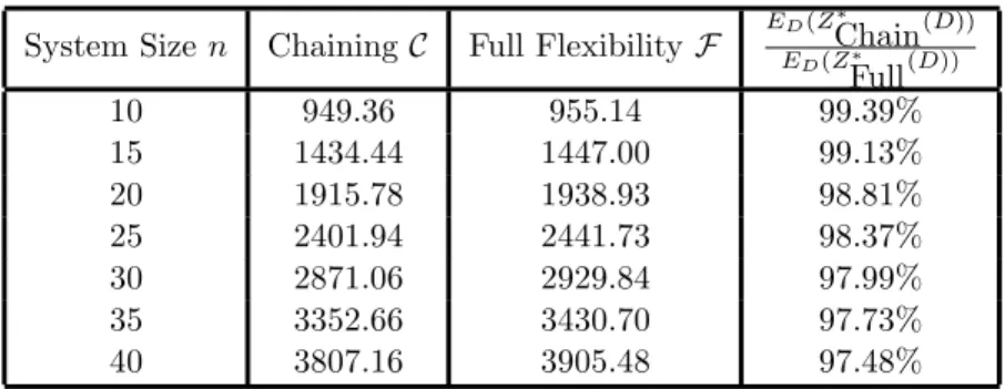
This implies that a simple chain structure can capture close to 90% of the value of the max flow in a fully flexible system, even when the system size is very large and the demand is uniform over a range. The performance in the case of normal distribution is even more impressive. Assuming that µ = 3σ, Table 1 shows the expected performance of two different structures over the random demand as n varies. For small n (say n = 10), their simulation shows that

System Sizen ChainingC Full FlexibilityF ED(Z ∗ Chain(D)) ED(Z∗ Full(D)) 10 949.36 955.14 99.39% 15 1434.44 1447.00 99.13% 20 1915.78 1938.93 98.81% 25 2401.94 2441.73 98.37% 30 2871.06 2929.84 97.99% 35 3352.66 3430.70 97.73% 40 3807.16 3905.48 97.48%

Table 1: Expected Sales and Chaining Efficiency for Increasing System Size

the expected sales, essentially the maximum flow, in the two systems are 949.36 and 955.14 respectively. This demonstrates that chaining already achieves most (99.39%) of the benefits of full flexibility in this case. As the system size expands, the performance of chaining deteriorates slightly, but still at an impressive level of 97.48% for n= 40. As n approaches infinity, it can be shown that the limit tends to a value close to 96% (cf. Chou et al. (2007a)).

The result of Jordan and Graves (1995) is important and exciting because it is consistent with a widely observed phenomenon: a simple and easy-to-execute structure (e.g. a chain structure) could be as good as the most complicated one (e.g. a full flexibility structure). It is thus reasonable to believe that a systematical and effective method to design a good sparse flexible structure can be adopted to applications in many different fields.

Bassamboo et al. (2008) extended the theory of chaining into dynamic processing system, through a concept called “tailored pairing.” Pairing is a configuration such that every two classes of demands are linked by exactly one resource, and hence is different from the concept of chaining, where there is a circular ordering of nodes and only adjacent demand nodes are linked by a resource. They used Brownian motion approximation to show that subject to mild conditions on the marginal cost structure as a function of the level of flexibility, tailored pairing is optimal for symmetric system (when average demand and supply are identical and balanced) in the heavy traffic regime. i.e., there is no need in the optimal solution to invest in server capable of serving three or more classes of demands. The authors further postulated that the same holds even for asymmetrical system, and supported their claims via numerical simulation.

2.2 Theoretical Results: Worst Case Performance

approach. They adopt the concept of graph expansion (Bassalygo and Pinsker (1973)), which is widely used in the area of graph theory and computer science (Sarnak (2004)), to study the process flexibility problem in this setting. Their study reveals the intimate connection between process flexibility and graph connectivity, and shows that the graph expander structure (i.e. a class of highly connected graphs with far smaller number of arcs than complete graph) works extremely well as a sparse flexibility structure. This result holds in many classes of objective functions, only requiring a mild assumption that the demand is bounded around its mean. i.e., demand is never more than a constant times of its mean.

Definition 1 D˜i has bounded variation of λaround its mean ifD˜i ≤λE[ ˜D] almost surely.

It turns out that when demand does not deviate substantially away from the mean, we can use the action flexibility inherent in the process structure to effectively allocate capacities to the demands. To do so, we need to understand the notion ofgraph connectivityassociated with every process structure.

Definition 2 A structure F is k-connected if there are at least k node disjoint paths linking every pair of nodes inA ∪ B.

Ak-chain (denoted byCk) is a subgraph in anbynbipartite graph where each supply node

i is linked to demand nodes i, i+ 1, . . . , i+k−1 (modulo n). The structure C_k is clearly k -connected, withknlinks. However, there are exponentially many classes ofk-connected graphs with kn edges, for k > 2, although the 2-chain is the only 2-connected graph with 2n edges. There is a clear trade-offs in the level of connectivity with the number of edges - for higher graph connectivity, the structure needs to have more edges.

There is a class of highly connected graph, calledgraph expander, which has received a lot of attention in the literature. Basically, graph expanders are graphs where every “small” subset of nodes are linked to a “large” neighborhood. The ratio of the size of the neighborhood and the size of the subset measures the expansion capability of the graph. We define the neighborhood of a subset and the concept of a graph expander formally in the following:

Definition 3 Let F be a bipartite graph with partite setAandB. ForS ⊂ A, the neighborhood of S in F is defined to be

Definition 4 Let F be a bipartite graph with partite set A and B. The structure F is a (α, λ,∆)-expander if

• for each node v in the graph, deg(v)≤∆ for everyv ∈ A, and

• for all small subsetS ⊂ A with |S| ≤αn, we have

|Γ(S)| ≥λ|S|.

Remark:

1. For a n×n bipartite graph which is also a (α, λ,∆)-expander, , the number of edges is at most ∆n.

2. A 2-chainC₂is clearly a (_n1,2,2) expander, since for each subset of size 1, there are at least 2 neighbors. Furthermore, the degree is bounded by 2. It is also a (2_n,1.5,2) expander, since for every subset S of size at most 2, |Γ(S)| ≥ 1.5|S|. It is easy to check that it is simultaneously a (k_n,(k+ 1)/k,2) expander, for allk≤n−1.

3. The reason why graph expander works well in matching supply and demand is because graph expander ensures that any suitably small group of product nodes is connected to a relatively large number of plants. Moreover, the notion that a long chain is better than a short chain can be cast in the same light: the expansion ratios for “small” subsets of product nodes in long chains are higher than that in short chains.

Chou et al. (2007b) established the following main result:

Theorem 1 Consider a n×n system, where the demand D˜i has bounded variation of λwith mean µi = µ. Assume that each plant has capacity µ. Let F be an (α, λ,∆)-expander, with

α×λ= 1− for some >0. Then

Z_F∗(D) ≥αλn " min µ, P i∈AD˜i n !# = (1−)Z_Full∗ (D) for all D.

Note that the -optimality performance holds for all demand scenario D, and is thus the

worst caseperformance of the expander structure, given that the demand has bounded varia-tion ofλ. This result is considerably stronger than the average case performance of the chaining

structure. Since 2-chainC₂in anbynbipartite graph is a (n−1_n ,_nn₋₁,2)-expander, we have the following immediate corollary:

Corollary 1 Suppose that (i) the demand of each product has bounded variation of 1 + _n−11 , (ii) with mean µi =µ, i= 1, . . . , n, and (iii) each of the nplants has capacity µ. Then

Z_C∗

2(D) =Z ∗

Full(D)

for all D.

Remark: We notice that truncated normal distribution is often used to model product de-mand distribution in a lot of service and manufacturing settings. When σ=µ/3, and demand is truncated at one standard deviation above the mean, then according to the above, 2-chain is always as good as the fully flexible system when n= 4. However, when nincrease, the worst case performance of a 2-chain is worse off compared to the fully flexible system.

In the worst case setting, the level of flexibility needed in the structure depends on the magnitude of demand deviation above the mean (i.e. level of uncertainty), which corresponds to the graph expansion ratio (parameter λ) in the expander structure. For k-chain, this ratio depends onn, and hence the performance ofk-chain suffers asnincrease. To find good process structure for large n, we use a different class of graph expander structure. In particular, we use expander where the number of edges can bemuch smaller than the number of edges in a fully flexible system. The existence of such structure is well known and is by now a folklore in the graph theory community.

Theorem 2 [Asratian et al. (1998)] For any n, λ≥1, andα <1 with αλ <1, there exists a (α, λ,∆)-expander, for any

∆≥ 1 + log2λ+ (λ+ 1) log2e

−log₂(αλ) +λ+ 1. (5)

Note that the lower bound on the degreee ∆ is independent of n, and hence the number of edges in this class of graph expanders is linear inn. The implication for the process flexibility problem can be stated more succinctly as follows:

In the symmetrical system, for any given demand distribution with bounded variation

λ, we can find a corresponding α with

αλ≈1−, for some >0,

such that for n sufficiently large, we can always find a process structure using at most ∆n edges, where ∆ is given by the right hand side of (5), such that the worst case performance of the structure is at most1−times of the fully flexible system. For more general system (i.e. the number of product nodes and plant nodes might be different and products follow different demand distributions), Chou et al. (2007b) proposed a generalization using the concept of “Ψ-expander”, with a high Ψ (0 < Ψ ≤ 1). Suppose the demand with meanµiis assumed to be bounded in [λi(U)µi, λi(U)µi]. We say that the demand has bounded variation ofλi(L) and λi(U) in this case.

Definition 5 A Ψ-expander in the process flexibility problem is a bipartite graph inA × Bwith

X j∈Γ(S) Cj ≥min    X i∈S λi(U)µi,Ψ X j∈B Cj − X i /∈S λi(L)µi   ,

for all subset S ⊆A.

The definition of Ψ-expander partitioned the subsets of Ainto two sets: (i) Forsmall subsetS

such thatP_i∈Sλi(U)µi+Pi /∈Sλi(L)µi≤ΨPj∈BCj, we have

X j∈Γ(S) Cj ≥ X i∈S λi(U)µi,

and hence the plants supplying to the small subsets have sufficient capacity to deal with demand arising from the small subset. (ii) At the same time, the capacity connected to a non-small subset is also large enough, i.e.

X j∈Γ(S) Cj ≥Ψ X j∈B Cj − X i /∈S λi(L)µi,

so that at least Ψ proportion of the total capacity is utilized in the worst case. It is thus easy to see that a structure with Ψ = 1 is as good as full flexibility.

Theorem 3 (Chou et al. (2007b)) Let F be a Ψ-expander. When D˜i has bounded variation

λi(L) andλi(U), then for all demand realization, we can find a solution forZF such that either

(a) all the plants are operating below their configured capacity level (because of insufficient demand), or (b) at least Ψ proportion of the total pre-configured capacity have been utilized.

The above theorem suggests that a Ψ-expander has the following nice property - as long as the demand for each product falls in the rangeλi(L)µi andλi(U)µi, then the process structure guarantees a utilization rate of 100×Ψ% in the entire system!

Example: Consider the process flexibility problem with 5 plants and 5 products. The capacity at each plant is 100 units, whereas the demand for the 5 products are between 50 and 150, each with mean of 100. Note that we did not specify the precise structure of the demand distributions. A fully flexible system in this case contains 25 edges, whereas a 2-chain has only 10 edges. Note that the demand is always within 1.5 times of its mean. Hence the 2-chain has bounded variation with λi(L) = 0.5, and λi(U) = 1.5. It can then be shown easily that the 2-chain is a 1-expander. Thus the 2-chain structure in this case has the sameperformance as the fully flexible system, for all demand realization! 2

2.3 Theoretical Results: Randomized Performance

The structural results in the worst case setting provides a glimpse to the structure of good process structure. However, for more complicated cases (such as the non-identical and asym-metrical demand setting), such structural insights may not be readily available. Instead of focusing on the performance of a specific structure, we can also study theaverageperformance of a class of process structures. This route of analysis allows us to examine the performance of “sparse” structures in other classes of design problems. To this end, we need to generalize the notion of process flexibility.

Consider the problem

(P) : Z(b,{1, . . . , n}) = max _Xn i=1 cixi:Ax≤b; xi ≥0, i= 1, . . . , n .

The dual problem is given by

(D) : Z(b) = min _Xm j=1 bjyj :ATy≥c; yj ≥0, j = 1, . . . , m . 2

One of the authors have often played a game with students in class - the students can choose demand values of any kind, as long as each value falls in the range of [50,150]. The instructor will then compare the performance of a 2-chain and a fully flexible system. Most students are amazed that a simple 2-chain always achieved the same performance as the complicated fully flexible system.

(D) is a linear programming problem with m variables and n constraints. If we sample N

constraints from (D), and denote the constraints sampled byS, we obtain the problem

(D(S)) : Z(b, S) = min _Xm j=1 bjyj :ATSy≥cS; yj ≥0, j = 1, . . . , m .

The dual of this problem is

(P(S)) : Z(b, S) = maxX i∈S

cixi :ASxS≤b; xi ≥0, i∈S

.

Let x∗(b) denote an optimal solution in Z(b,{1, . . . , n}). Note that since b is random, x∗(b) is also a random vector. We assume that problem (P) has an optimal solution x∗(b) with the following property:

(Property A): x∗_i(b)≤λE_b(x∗_i(b)) almost surely for some constant λ >0 (independent of

n), and for all i= 1, . . . , n.

The above property essentially states that for each realization of b, the optimal primal solution x∗(b) should not be too far above its mean value. This is similar to the bounded variation assumptions in the process flexibility problem.

Theorem 4 Suppose Property A holds for (P). Then there exists a set S with cardinality

N =O(λm ), such that

Eb(Z(b, S))≥(1−)Eb(Z(b)).

In the case whenn >> m,S is considered a sparse set and plays the role of the sparse structure in the process flexibility problem. This theorem identifies a natural condition under which we can expect a suitably chosen sparse subsetS (withO(m) variables) to “perform” nearly as well as a fully flexible system withn variables, even ifn >> m.

To construct the sparse set S with near optimal performance, we need to understand the behavior of the (random) optimal solutionx∗(b). The setSin the above theorem is constructed by repeatedly sampling from the distribution x∗(b), up to O(λm ) times. We will see in the later sections that for several classes of problems, the optimal solution x∗(b) can be obtained in closed form. For the technical details pertaining to this result, we refer the readers to Chou et al. (2007a).

3

Construction Methods

The process flexibility problem can be technically modeled as a two stage stochastic program-ming problem, where the first stage decision concerns the selection of links subject to budget constraints (0-1 discrete problem), whereas the second stage problem concerns finding the best recourse action to match supply with demand, to obtain the expected second stage cost function arising from the optimal recourse decisions. The latter is a difficult problem, since it involves finding the expected maximum flow problem (or worst case max flow) in a general bipartite graph. While there are numerical methods that can be used to handle this kind of problems when the size is small, it is not widely used in practice, due to the difficulty in finding reli-able distributional information on demand and accurate cost estimation. To the best of our knowledge, this algorithmic design problem has also been largely overlooked by the research community, in part due to the technical difficulties associated with this problem.

We describe next several heuristics that can be used to construct good process structure quickly, exploiting the structural insights discussed in the previous section. We also review a recent approach to address this problem, using the theory of robust optimization.

3.1 Chaining Method

The chaining concept (Jordan and Graves (1995)) is arguably the most influential strategy used in practice to design good process structure. It is developed based on two key insights obtained from Jordan and Graves (1995)’s landmark study:

• By adding a small amount of flexibility at the proper places in an otherwise rigid system, we could achieve a significant improvement in its performance; and

• the links should be added to the structure to obtainlong chains.

A chain refers to a path which goes through a group of distinct product and plant nodes in consecutive order, returning to the start node at the end to form a cycle. A long chain is preferred because it has the ability to pool the plants’ capacity and products’ demand together and thus can deal with demand uncertainties more effectively than a short chain.

Based on the above conceptual ideas, Jordan and Graves (1995) provided three other general guidelines to design process structure. They advise the designer to

• try to equalize the capacity allocated to each product node in the chain;

• try to equalize the expected demand allocated to each plant node in the chain;

• construct a long circular chain visiting as many nodes as possible.

The first two guidelines aim to help the plants to achieve higher capacity utilization and to satisfy more demand. In the symmetric case, with each product and each plant having the same level of mean demand and capacity, we can use the three guidelines to obtain a regular 2-chain.

The above guidelines are obtained and validated by extensive numerical simulation results. However, these guidelines alone do not provide an implementable heuristic which can be used to design a process structure. Jordan and Graves (1995) mentioned that they have no firm guidelines to adding flexibility for more general cases. In fact, in their work, they use the guide-lines they developed to obtain various process structures, and then used numerical simulation to estimate the performance (e.g. average lost sales; unused capacity at each product and plant etc.) of each structure, to determine the best process structure. This process is tedious and time consuming. The next method tries to address this deficiency, using a heuristic guided by the graph expansion concept.

3.2 Node Expansion Method

The previous section shows that the performance of a process structure is intimately connected to its underlying connectivity property. We can thus design a good process structure by con-structing a graph with good expansion ratio. The latter problem is recently investigated by Ghosh and Boyd (2006). However, their approach works more for the symmetrical case (graph expansion is after all a concept originating in graph theory), but does not address the issue associated with asymmetrical supply and demand setting.

The notion of graph expansion is nevertheless connected to the design guidelines popularized by Jordan and Graves (1995). The first and second guideline seek to equalize the capacity and expected demand allocated to each product and plant respectively. This is related to the concept of expansion ratio for all (small) subsets containing only a single node. We extend this strategy further by fully exploiting this connection.

The node expansion method works by checking the expansion ratio of all singletons, although the method can be easily extended to handle all subsets with up to k (k fixed, small) nodes. Starting from any rigid base structure, the method augments the structure by adding links iterativelyto improve upon the node expansion ratio in a greedymanner:

In each iteration, we add a link connecting the product node with the lowest product expansion ratio (i.e. the ratio of the total capacity of the connected plants to the product’s expected demand), to the plant node with the lowest plant expansion ratio (i.e. the ratio of the total expected demand of the connected product nodes to the plant’s capacity). We skip this edge if it has already been added to the structure, and move to the plant node with the next smallest expansion ratio. We repeat this procedure until the number of added links reached the pre-determined limit.

Simulation studies by Chou et al. (2007b) show that this design heuristic can generate good process structures in several applications. In fact, on the process flexibility problem encountered in GM, the structure obtained using this direct constructive approach is already as good as the structure developed by Jordan and Graves (1995) guided by extensive numerical simulation. We refer the readers to Chou et al. (2007b) for details.

3.3 Sampling Method

The sampling method builds on Theorem 4. For the process flexibility problem, the optimal solution is trivial under the full flexibility structureF. Note that in this problem, with demand

D = (D1, D2, . . . , Dm) and capacity C = (C1, . . . , Cn), the max flow problem ZF∗(D) has up

to nm variables, with onlyO(n+m) constraints. There are multiple optimal solutions to this simple problem, and the properties of the extreme point solutions are well known. For our purpose, however, we need a closed form solution to the problem. Fortunately, this is easy when the structure corresponds to the full flexibility structureF.

Lemma 1 In the process flexibility problem,

x∗_ij(D) = DiCj max Pm i=1Di, Pn j=1Cj , i= 1. . . m, j = 1, . . . , n,

is an optimal solution to Z_F∗(D) under the full flexibility structure F. Furthermore, Z_F∗(D) = min _Xm i=1 Di, n X j=1 Cj .

Using this solution, we can construct (random) process structure by sampling arc (i, j) with probability proportional to x∗_ij(D). The sampling heuristic basically has two stages.

• In the first stage, the sampling probability for each link (i, j) (i= 1. . . m, j = 1. . . n) is estimated by calculating the empirical average of the flow on the arc (i, j). This is used in the case when x∗_ij(D) does not have an easy closed form expression.

• In the second stage, structures can be created by selecting links using the estimated sampling probabilities, and the structure with the best performance will be ultimately selected.

Note that the sampling method uses numerical simulation to obtain the performance of the structure sampled, and in a way, this is identical to the approach used by Jordan and Graves (1995). The advantage of the sampling method is that it is systematic, and can be applied to a wide variety of other problems, ranging from capacity pooling networks (Chou et al. (2007a)) to transshipment network design (Lien et al. (2005)). The disadvantage, on the other hand, is that the sampling method cannot ensure that every structure sampled will be good, and an additional evaluation step (e.g. through simulation) is needed to identify a good structure. Furthermore, although the method works theoretically, we do not have good qualitative understanding of the features inherent in near optimal sparse structures.

3.4 Robust Optimization

The process flexibility problem can be recast as a two-stage stochastic maximum flow problem as follows: max_x EP h Q(ξ˜,x) i s.t. X i xi=K, xi∈ {0,1},

whereK represent the maximum number of links in the process structure,xthe design decision variables, and ξ˜denotes the random demand parameters in the problem, with distribution P.

The recourse function is given by:

Q(ξ˜,x) =Z_G(∗_x)(D) s.t. ξ˜=D,

e∈ G(x) if and only ifxe = 1.

When the probability measure on the scenario space is not explicitly given, we can minimize the worst case performance of the design, over an uncertainty set U, to obtain a robust two stage maximum flow problem:

max_x min ˜ ξ∈U h Q(ξ˜,x) i s.t. X i xi=K, xi∈ {0,1},

To solve this robust optimization problem, the challenge is to find a nice uncertainty setU, so that the problem

max_x t

s.t. X

i

xi=K, xi∈ {0,1},

t≤Z_G(∗ _x)(ξ˜)∀ ξ˜∈ U.

can be recast as a tractable convex optimization problem, even if the set U has infinitely many scenarios. Unfortunately, whenU represents the set of demand scenarios with bounded variation around the means, the above robust formulation can be solved in polynomial time if and only if P = N P. We refer the readers to details in Atamturk and Zhang (2007), and for some special cases when the robust two stage network design problem can be solved in polynomial time. The currently available approach to solve the robust process flexibility problem is via the cutting plane approach, and is thus not computationally efficient.

4

Measurement and Evaluation

The research on the evaluation of process flexibility has so far focused on creating indices to rank process flexibility structures, in terms of level of flexibility inherent in the structure. This line of pursuit complements the constructive approaches, and seeks way to allow the managers to compare different process structures quickly, without the need to evaluate its performance in simulation, due to the lack of cost parameters and/or distributional information on the uncertain parameters. The computation of the indices uses minimal information on the uncertain demand parameters (mostly average values). These indices are thus usually easy-to-compute, and can

effectively rank the structures in terms of performance, though they cannot give an absolute value of the performance of the different process structures.

4.1 JG Index

Jordan and Graves (1995) developed a probabilistic index to measure the performance of a given structure. For any subset S of demand nodes, they focus on the probability that the unsatisfied demand in that structure would exceed that for the corresponding full flexibility structure. i.e., PX j∈S Dj− X i∈Γ(S) Si ≥max 0,X j Dj − X i Si .

The largest probability among all subsets is used as a flexibility index to compare among structures. A good flexibility structure should have a low index, since a more flexible structure should deal with demand uncertainty more effectively, and thus the unfilled demand of the structure should be as close to the full flexibility structure as possible. However, the JG index is usually very hard to compute.

4.2 Structural Flexibility Index

The index developed by Iravani et al. (2005) is arguably a milestone in the development of a measure for process flexibility. In this study, a suitably defined “structural flexibility matrix” (SF Matrix) M was proposed to calibrate the performance of a process structure. An entry (i, j) inM, denoted by M(i, j), represents the

maximum number of non-overlapping routes from demand node i to demand node

j, whereas

M(i, i) = degree of arcs connected to the demand node i.

The largest eigenvalue and mean of the entries in SF matrixM are used as two alternate indices to determine the level of flexibility in a process structure. SF indices are much easier to compute and work better than probabilistic indices in many examples (cf. Iravani et al. (2005)), although the computation of each entry in the matrix requires solving a maximum flow routine.

4.3 Expansion Index

We propose an alternate index to measure the performance of a process structure, using the observation that graph with higher connectivity tends to be more flexible, which has been theoretically verified in the balanced and identical case. Let N denote the number of nodes (including both supply and demand nodes), and L the number of links in the structure. The expansion index is defined as the second smallest eigenvalue of the Laplacian matrix

L=T T0,

whereT is a N×L matrix. For linkl connecting nodei∈A(with mean µi) andj ∈B (with mean Sj), the corresponding entry in column l ofT is

T_il =pµiSj, Tjl=−

p

µiSj, and Tkl= 0, ∀k6=i, j.

The index is developed using a well-known observation in graph theory that the second smallest eigenvalue of L, i.e. λ2(L), is a good surrogate for measuring the connectivity of the

underlying graph (see Fiedler (1973), Ghosh and Boyd (2006)) in the case when µi =Sj = 1 for all i, j. As shown in the earlier section, a graph with good expansion ratio (high λ2(L))

is highly connected and is more flexible in matching supply and demand. λ2(L) can thus be

used as an alternate index to rank process structures. The indexλ2(L), as compared to the SF

indexM, has the key advantage that it has been thoroughly studied in the literature.

4.4 Numerical Comparison

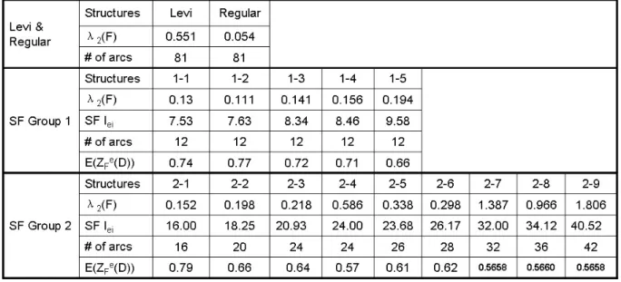
These indices have been tested in the following numerical experiments. The first experiment is to rank the performance of two different graphs, i.e., the Levi graph and the regular 3-chain (cf. Figure 6). Both graphs are regular with degree 3, and hence have equal number of edges. The Levi graph has slightly better expansion ratio for small subsets up to order 3. In fact, it can be shown that each subset of order 3 on one side has at least 5 neighbors, whereas it is easy to find subsets of order 3 in the 3-chain with only 4 neighbors.

As shown in table 2,λ2(Levi) (0.55) is higher thanλ2(Regular) (0.05), in the symmetric case

when all demand means and capacity levels are identical. This indicates that the Levi graph could be a better process structure than the 3-chain. This is consistent with our simulation

A B C D E F G H I J K L M N O P Q R S T U V W X Y Z A A 1 2 3 4 5 6 7 8 9 10 11 12 13 14 15 16 17 18 19 20 21 22 23 24 25 26 27 A B C D E F G H I J K L M N O P Q R S T U V W X Y Z A A 1 2 3 4 5 6 7 8 9 10 11 12 13 14 15 16 17 18 19 20 21 22 23 24 25 26 27

A : A levigraph B : A regular graph

Figure 6: Levi graph and a regular chain with degree 3.

experiments: the Levi graph can indeed support slightly higher amount of flow in the process flexibility problem, compared to the 3-chain, for a variety of demand distributions.

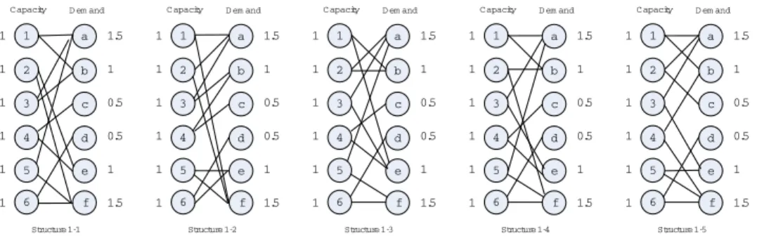
We have also evaluated the performance of the expansion indices and SF indices, using two representative examples studied in Iravani et al. (2005). The first example is a group of struc-tures with random demand µ = (1.5,1,0.5,0.5,1,1.5) and fixed capacity S = (1,1,1,1,1,1) (c.f. figure 7). The second example is a group of structures with random demand µ = (1,1,1,1,1,1,1,1) and fixed capacity S = (1,1,1,1,1,1,1,1), as shown in figure 8.

We useE(Z_Fe(D)), the expected excess flow in structureF, as the benchmark to evaluate the performance of structureF. E(Z_Fe(D)) is closely related to the max-flow objective E(Z_F∗(D)), because the excess flow Ze

F(D) is simply

Pn

i=1Di −ZF∗(D), the amount of unmet demand.

E(Z_Fe(D)) is a better benchmark for this experiment because it is more sensitive and does not scale as much as the max-flow objective when problem size changes. We approximateE(Ze

F(D)) by sampling 200 demand scenarios, each with demandDi uniformly distributed in (0, 2µi).

In both cases, the ranking obtained from the expansion index is consistent with the ranking given by (the empirical average) E(Z_Fe(D)). The ranking given by SF index, on the other

1 4 3 2 5 6 a d c b e f 1 1 1 1 1 1 1.5 1 0.5 0.5 1 1.5 C apacity D em and Structure 1-1 1 4 3 2 5 6 a d c b e f 1 1 1 1 1 1 1.5 1 0.5 0.5 1 1.5 C apacity D em and Structure 1-2 1 4 3 2 5 6 a d c b e f 1 1 1 1 1 1 1.5 1 0.5 0.5 1 1.5 C apacity D em and Structure 1-3 1 4 3 2 5 6 a d c b e f 1 1 1 1 1 1 1.5 1 0.5 0.5 1 1.5 C apacity D em and Structure 1-4 1 4 3 2 5 6 a d c b e f 1 1 1 1 1 1 1.5 1 0.5 0.5 1 1.5 C apacity D em and Structure 1-5

Figure 7: SF Group 1: Structures with Demand µ= (1.5,1,0.5,0.5,1,1.5)

1 4 3 2 5 6 a d c b e f 1 1 1 1 1 1 1 1 C apacity D em and Structure 2-3 7 8 g h 1 1 1 1 1 1 1 1 1 4 3 2 5 6 a d c b e f 1 1 1 1 1 1 1 1 1 1 1 C apacity D em and Structure 2-4 7 8 g h 1 1 1 1 1 1 4 3 2 5 6 a d c b e f 1 1 1 1 1 1 1 1 1 1 1 C apacity D em and Structure 2-5 7 8 g h 1 1 1 1 1 1 4 3 2 5 6 a d c b e f 1 1 1 1 1 1 1 1 1 1 1 C apacity D em and Structure 2-6 7 8 g h 1 1 1 1 1 1 4 3 2 5 6 a d c b e f 1 1 1 1 1 1 1 1 1 1 1 C apacity D em and Structure 2-7 7 8 g h 1 1 1 1 1 1 4 3 2 5 6 a d c b e f 1 1 1 1 1 1 1 1 1 1 1 C apacity D em and Structure 2-8 7 8 g h 1 1 1 1 1 1 4 3 2 5 6 a d c b e f 1 1 1 1 1 1 1 1 1 1 1 C apacity D em and Structure 2-9 7 8 g h 1 1 1 1 1 1 1 4 3 2 5 6 a d c b e f 1 1 1 1 1 1 1 1 1 1 1 C apacity D em and Structure 2-1 7 8 g h 1 1 1 1 1 1 4 3 2 5 6 a d c b e f 1 1 1 1 1 1 1 1 C apacity D em and Structure 2-2 7 8 g h 1 1 1 1 1 1 1

hand, are slightly different from (the empirical average) E(Z_Fe(D)). Note that lower value of

E(Z_Fe(D)) should ideally correspond to higher index value. Unfortunately, the SF method errs on the performance of 1-1 and 1-2, and on 2-4 vis-`a-vis the rest. The simulation results indeed suggest that both the expansion index and SF index are easy-to-compute indices that can be used to rank process structures rather effectively.

Table 2: Comparisons among Flexibility indices

5

Applications

The central theme in this paper is the observation that a little flexibility can go a long way in enhancing the performance of the system. We have discussed the impact of this phenomenon on the process flexibility problem in the earlier sections. This insight has also been observed in numerous other settings. In the rest of this section, we review some of the key results obtained for other related areas, and discuss some new applications.

5.1 Multi-Stage Supply Chain

Graves and Tomlin (2003) extended Jordan and Grave’s work to multi-product, multi-stage supply chains, where each product needs to flow through several stages in the supply chain. They proposed a supply chain flexibility measureg, where higher g indicates higher flexibility. Unfortunately, they stop short of offering a method to design a flexible supply chain network.

The results established in the earlier sections can be used to establish a much stronger result concerning the performance of sparse supply chain structure. We also give a glimpse of the performance of the sampling method using this example as an illustration.

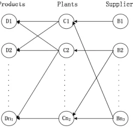
Consider the following supply chain design problem (see figure 9): There are n1 products,

n2 plants, and n3 suppliers. In the full flexibility scenario, each product can be produced at

any plant, using material source from any of the supplier. We assume that each unit of product consumes a unit of material from each supplier and uses a unit capacity at a plant. We assume further that production capacity at the plants are Ci, i = 1, . . . , n1, and the suppliers have

limited amount of materials, at capacity Bi, i = 1, . . . , n3. The demand for each product is

random and denoted by the random variable Di, i= 1, . . . , n1.

Figure 9: A Supply Chain Flexibility Structure.

In the full flexibility scenario, it is easy to see that the expected sales is given by

ED min Xn1 i=1 Di, n2 X i=1 Ci, n3 X i=1 Bi .

The above problem can be formulated as the following set packing problem: Z∗(D) = max n1 X i=1 n2 X j=1 n3 X k=1 xijk s.t. n2 X j=1 n3 X k=1 xijk ≤Di ∀i= 1,2, . . . n1; (6) n1 X i=1 n3 X k=1 xijk ≤Cj ∀j= 1,2, . . . n2; (7) n1 X i=1 n2 X j=1 xijk ≤Bk ∀k= 1,2, . . . n3; (8) xijk ≥0 ∀i, j, k. (9)

For each realization of demand Di, it is easy to see that there is an optimal solution given by xijk(D) = DiCjBk max Pn1 i=1Di×Pnj=12 Cj,Pni=11 Di×P_kn₌₁3 Bk,Pnj=12 Cj×Pn_k=13 Bk .

Let S = {(i, j, k) : material from supplierk used to produce productiat plantj} denote the supply chain configuration. We have an analogous result for this problem setting.

Theorem 5 Suppose the demand distribution satisfies

xijk(D) = DiCjBk max _P n1 i=1Di× Pn2 j=1Cj, Pn1 i=1Di× Pn3 k=1Bk, Pn2 j=1Cj × Pn3 k=1Bk ≤ λE DiCjBk max Pn1 i=1Di×Pnj=12 Cj,Pni=11 Di×P_kn₌₁3 Bk,Pnj=12 Cj×Pn_k3₌₁Bk ,

for some λ >0, then there exists a sparse supply chain configuration S with cardinality |S| =

O(λ(n1+n2+n3)/), such that the expected demand met by the sparse supply chain system is

at least (1−)E(Z∗(D)).

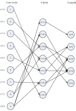
We can use the sampling method to obtain good sparse supply chain structure. Consider a supply chain with 9 products, 7 plants and 5 suppliers. Demand for each product is normally distributed. The expected demands are shown in figure 10. The standard deviation is 40% of the expected demand. Products can be divided into 3 subgroups. Demands of products in the same subgroup are correlated. The correlation coefficients are 0.2 pairwise in subgroup 1

(product 1 to 4), -0.2 pairwise in subgroup 2 (product 5 to 7), and 0.1 in subgroup 3 (product 8 and 9). There are no correlations between demands of products in different subgroups. Supplies from the suppliers are also normally distributed. For each supplier, the standard deviation is 40% of the expected supply (shown in figure 10). Each plant is able to produce any product. The capacity of each plant is fixed (see figure 10). In the full flexibility scenario, a plant can produce any product using the material supplied by any supplier.

1 2 3 4 6 7 8 9 5 C=1.3 C=4.7 C=8.6 C=11.7 C=8.3 C=6.3 C=13.4 S=8 S=6 S=19 S=12 S=10 D em ands Plants Supplies

µ=7.6 µ=5.7 µ=7.4 µ=5.1 µ=4.5 µ=2.1 µ=3.6 µ=7.3 µ=8.9

Figure 10: A Supply Chain Network with N=12, obtained from the sampling approach.

We conduct a simulation study to test whether there exists a partial flexible supply chain network capturing almost all the benefits of the full flexibility system. We simulate 100 scenarios of demands for each retailer and 100 scenarios of supplies for each supplier. We use the number of paths in the network to denote the degree of flexibility. For each degree of flexibility (N from 10 to 315) we generate 100 structures using the sampling method and return the structure with the best empirical performance.

Figure 11 shows the effect of higher degree of flexibility on the expected sales. The figure shows that the marginal contribution of every additional path is in general diminishing in its returns on expected sales. When 10 paths are selected, the expected total sales is already 85%

38 40 42 44 46 48 50 10 11 12 13 14 15 16 17 18 19 Fu llF lexi bili ty

Supply C hain Structures

E x p e c te d S ta ti s fi e d D e m a n d

Figure 11: Expected Satisfied Demand as Flexibility Increase.

of the expected sales under the full flexibility system. After the number of paths is increase to 19, the total sales is a whopping 99% of the expected sales in the full flexibility system (with a total of 315 paths).

5.2 Military Deployment and Transshipment

Inspired by the defense in depth strategy devised by Emperor Constantine (Constantine The Great, 274-337), Revelle and Rosing (2000) studied the following problem in troops deployment: Each region in the empire must be protected by one or more mobile field armies (FAs) to throw back invading enemies. It is secured if one or more FAs is stationed in the region. It is securable if an FA can reach the region in a single step (i.e., there is a route linking the region where the FA is stationed to it). However, an FA can be deployed from one region to another adjacent region only when there is at least one other FA to help launch it. i.e., the FA must come from a region with at least two FAs stationed in it. This restriction is much like the island hopping strategy used by General MacArthur in World War II in the Pacific.

The puzzle confronting Emperor Constantine concerns the positioning of 4 FAs to protect the 8 regions in his empire as shown in Figure 12. He chose to position two FAs at Rome, and two at his new capital Constantinople, leaving the outskirt region Britain vulnerable to enemies’ attack. By focusing on the troops deployment problem in the event of war in one of the regions, Revelle and Rosing (2000) solved the above puzzle by formulating the problem into

Figure 12: The empire of Constantine.

an integer program. In this case, all the regions in the empire can be protected by stationing one FA in Britain, one in Asia Minor, and two in Rome.

Note that the above deployment, however, is not securable in the event that two or more wars happen at the same time. For instance, this deployment could not secure against joint outbreak of wars in any two of the five regions: Gaul, Iberia, North Africa, Egypt and Constantinople. A slightly better deployment is to station two FAs at Iberia, and another two FAs at Egypt. This secures the regions for up to two wars, except if the wars occur at Britain and Gaul, or Constantinople and Asia Minor. This deployment is thus more resilient against the joint outbreak of two wars. Unfortunately, this latter deployment is politically unacceptable as no troops are now stationed at the capital city Rome.

In general, finding the best deployment solution securing against outbreak of wars in up to

k regions (fork≥2) is a challenging problem. The minimum number of FAs needed to secure the regions will largely depend on the network structure for troops re-deployment. In general, if the network is dense (with many links joining different regions), or has one region connecting to many different regions, then the number of FAs needed will be low.

In this section, we consider an analogous military deployment problem. Consider a military mission, where n strategic locations need to be defended against possible enemy’s invasion. The army has Qi units of troops in location i. Unfortunately, the enemy’s mission could not be predicted, and the unit of troops deployed by the enemy to attack location iis denoted by

in location i may be deployed to location j, if the troops can be trained to rush from i to j

within stipulated time. Of course, it will be ideal to have many reinforcement paths, as that means the whole force can be pooled together at the right place to deal with enemy’s invasion. However, due to the limited time in deployment, each unit in location ican only be trained to reinforce limited number of other locations. The challenge is to design a reinforcement network to defend against the enormous number of enemy’s possible course of action.

This problem is similar to the transshipment problem studied in the literature, although the latter focuses mainly on the optimal inventory policy and optimal order quantity Q∗_i for each retailer (For problems with two retailers, see Tagaras and Cohen (1992); for problems with many identical retailers, see Robinson (1990)). They all assumed complete grouping, i.e., a retailer could tranship its products to any other retailers. Only a few papers discuss how to design a transshipment networks. Lien et al. (2005) studied the impacts of the transshipment network structure. They compared the performance of different network configurations: no transshipment, complete grouping, partial grouping, unidirectional chain and bidirectional chain (See Figure 13). Similar to the findings in Jordan and Graves (1995), they showed that sparse transshipment network structures can capture almost all the benefits of complete grouping. They also indicated that the chaining structure, which is also a kind of sparse structure, would outperform other sparse structures.

The troops deployment (and the transshipment) problem can be reduced to a variant of the process flexibility problem, where there arenplants andnproducts. Each plant ihas capacity (Qi−Di)+ (the left over at retailer i), which can be used to meet demand for other products. Each product has demand (Di−Qi)+(unfilled demand at retaileri). Note that in this case, both capacity and demand are random parameters in our problem, and (Qi−Di)+×(Di−Qi)+= 0. From Theorem 4, and the analysis therein, the existence of a sparse support structure for the troops deployment problem is guaranteed by the following condition:

x∗_i,j(D) = (Di−Qi) +_(Q j −Dj)+ max Pn i=1(Di−Qi)+,Pnj=1(Qj−Dj)+ ≤λED (Di−Qi)+(Qj −Dj)+ max Pn i=1(Di−Qi)+,Pnj=1(Qj−Dj)+

1 2 4 3 1 2 4 3 Complete Pooling A Bidirectional

Chain 1 2 4 3 Group Pooling 1 2 4 3 A Unidirectional Chain

Figure 13: Different Kinds of Transshipment Network Structures

Example: When Di are i.i.d. and take values in {0,2} with equal probability, Qi = 1 for all

i = 1, . . . , n, then (Di −Qi)+ and (Qi−Di)+ are Bernoulli variable with equal probability.

Note that E((Di−Qi)+) =E((Qi−Di)+) = 1 2. Furthermore, n X i=1 (Di−Qi)++ n X j=1 (Qj−Dj)+= n X i=1 |Di−Qi|=n. Hence x∗_i,j(D) = (Di−Qi) +_(Q j−Dj)+ max Pn i=1(Di−Qi)+, Pn j=1(Qj−Dj)+ ≤ 2 n(Di−Qi) + (Qj−Dj)+ ≤ 8 nE (Di−Qi)+(Qj−Dj)+ ≤ 8ED (Di−Qi)+(Qj −Dj)+ max Pn i=1(Di−Qi)+,Pnj=1(Qj−Dj)+ .