Extraction of main levels of a building from a large point cloud

(1)

EXTRACTION OF MAIN LEVELS OF

A

BUILDING FROM A LARGE POINT CLOUD

C.Leoni 1_{, S. Ferrarese} 1_{, W. Wahbeh} 2_{, C. Nardinocchi} 1

1_{DICEA, Sapienza University of Rome, Area Geodesia e Geomatica - Via Eudossiana 18, 00184 Roma, Italy} 2_{University of Applied Sciences and Arts Northwestern Switzerland School of Architecture, Civil Engineering and Geomatics}

Institut Digitales Bauen - Hofackerstrasse 30, 4132 Muttenz, Switzerland

[email protected]; [email protected]; [email protected]; [email protected]

Commission V, WG V/7

KEY WORDS: 3D Scanning Data, Scan-to-BIM, Subsample, Outliers, Plane Extraction, Robust Estimator, Positioning Levels.

ABSTRACT:

Horizontal levels are references entities, the base of man-made environments. Their creation is the first step for various applications including the BIM (Building Information Modelling). BIM is an emerging methodology, widely used for new constructions, and increasingly applied to existing buildings (scan-to-BIM). The as-built BIM process is still mainly manual or semi-automatic and therefore is highly time-consuming. The automation of the as-built BIM is a challenging topic among the research community. This study is part of an ongoing research into the scan-to-BIM process regarding the extraction of the principal structure of a building. More specifically, here we present a strategy to automatically detect the building levels from a large point cloud obtained with a terrestrial laser scanner survey. The identification of the horizontal planes is the first indispensable step to produce an as-built BIM model. Our algorithm, developed in C++, is based on plane extraction by means of the RANSAC algorithm followed by the minimization of the quadrate sum of points-plane distance. Moreover, this paper will take an in-depth look at the influence of data resolution in the accuracy of plane extraction and at the necessary accuracy for the construction of a BIM model. A laser scanner survey of a three floors building composed by 36 scan stations has produced a point cloud of about 550 million points. The estimated plane parameters at different data resolution are analysed in terms of distance from the full points cloud resolution.

1. INTRODUCTION

The creation of horizontal levels is the first step in many applications concerning 3D building reconstruction, such as those relative to the Building Information Model (BIM), since they are the main reference of a structure which host the building elements. In fact, BIM, widely used today for new constructions (Volk, 2014), is now being applied to existing buildings and known as built BIM. The automation of the as-built BIM process (Son et al., 2015) is a challenging topic. Commercial solutions (Faro, PointCab, Edgewise, CloudWorx) offer very useful semi-automatic approaches, but they are still time consuming. The research community currently focusses on automatic detection of walls, floors, windows, doors, roofs. The as-built BIM model is derived from a point cloud, mainly obtained by a terrestrial laser scanner survey, and therefore the process is called scan-to-BIM. It deals with a very complex problem: the need to generalize the survey and to generate an implicit model (Surfaces) out of an explicit model (point clouds). For example, how to handle in a BIM environment the approximation of the horizontality of a plane or the slight deviation of the orthogonality which arises between two walls? Problems that increase with the age of old building. Moreover, the automation of the scan-to-BIM process has to deal with a large amount of data. Building surveys require more and more scan stations to perform a good alignment and to avoid lack of data. In addition, a large amount of noise may be present, as often the survey is performed in a fully furnished building. Hence, plane extraction methods need to be very robust and efficient. Several have been described in literature and the two

most used for big data are: RANSAC ("RANdom SAmple Consensus") and Region Growing. Region growing was originally used in image segmentation (Zucker, 1976) and extended successively to point cloud. The principle of region growing is to create a region of connected points (or pixels) with a shared characteristic. Improved plane extraction algorithms based on region growing were subsequently introduced (Wang et al., 2016). While region growing is very fast in image segmentation, before applying to unstructured point cloud it requires a data organization to permit rapid access. RANSAC (Fischler and Bolles, 1981) is a very simple iterative procedure based on the following three steps:

1.three random points are extracted from the point cloud; 2.the direction numbers n : [a,b,c] of the plane defined by the

three points are calculated;

3.the number of points which are less than a certain distance from the plane is calculated.

The number of repetitions depend on the probability of finding the searched model in the data and on the presence of outliers in the point cloud. At the end the best plane is that with the greatest consensus (higher number of points within its threshold). RANSAC is widely used to detect and extract planes in laser scanning data due to its simplicity and robustness (Macher et al., 2016; Previtali et. Al, 2018; Thomson and Boehm., 2015). Improvements of the RANSAC algorithm were made to overcome difficulties in managing large point clouds (Yang, 2010; Subramaniam and Ponto, 2014, Lan et al, 2018). In (Tarsha-Kurdi et al., 2007; Oswald et al., Nguyen et al.,

The International Archives of the Photogrammetry, Remote Sensing and Spatial Information Sciences, Volume XLII-5/W2, 2019 Measurement, Visualisation and Processing in BIM for Design and Construction Management, 24–25 September 2019, Prague, Czech Republic

(2)

2017) are presented interesting comparative analyses between plane extraction methods.

This study is part of an ongoing research on the scan-to-BIM process. More specifically, we are working on a strategy to automatically detect the building level from a large point cloud derived from a terrestrial laser scanner survey. Level extraction is the first indispensable step to achieve an as-built BIM model. RANSAC is used to detect points on the same plane, then the direction numbers are estimated with a least square approach. The first results of point data segmentation are presented. All planes having a minimal dimension of 0.25m2_{are considered.}

The data set is about 250 million points and has a mean point space of less than 1mm. It is subsampled a variable resolution and segmented by level and by room.

The questions we pose are. First, which accuracy is necessary to appropriately model the data set. For instance, the rooms of a floor should be the same height, but this is true only within a certain threshold which depends on data accuracy and on floor inclination. In fact, floor and ceiling should be horizontal planes, but there is always an inclination. Second, which data resolution to use to work with a reduced point cloud without affecting the geometric results will also be assessed.

2. PLANE FITTING

The equation of a plane is represented by the general expression:

a x + b y + c z + d = 0 (1)

where a, b e c are the direction numbers of a unit normal vector n = [a, b, c]T _{under the condition that:}

(2)

and x, y, z are the coordinates of a point belonging to the plane. Given the set of points of a consensus set extracted from Ransac, the direction numbers of the plane are estimated minimizing the quadrat sum of the distance from each point to the plane. The orthogonal distances of the point Pi: [xi, yi, zi]T

with i: 1..N is:

(3)

And C: [xc, yc, zc]T_{is the centroid of all its points. Introducing a}

matrix M of dimension (N x 3), with the i-th raw containing the baricentric coordinates of the point Pi:

Mi : [ xi - xc; yi – yc; zi - zc] (4) 

We can express the quadrat sum of the distances as (Fienen., 2005):

(5)

The vector n that minimizes the relation is determined by the relationship or quotient (ratio) of Rayleigh, and is the minimum eigenvector corresponding to the minimum eigenvalue of A.

(6) This method performs the least square plane estimation solving an orthogonal matrix of the same dimension as the unknown. Parameter d can be estimated by mean the coordinate of the centroid as:

d = - a xc – b yc – c zc (7)

This method allows with a fast solution, even with a large number of points (we use it with until five million of points) to refine the plane parameters defined by the three points. The method is strongly dependent to outliers (Gašinec et al., 2014) but data used is free of outlier because it came from RANSAC algorithm. Residuals are calculated from the distances of points from the plane and from that is obtained the 0 of the solution.

3. MATERIAL AND METHODS 3.1 Data Set

The surveyed three-storey building has a total surface is 140 square meters. It has a regular square map and a roof hut.

Figure 1. Photographs of the exterior of the building.

The survey realized by Engineering Studio of Rieti (SCS Progetti s.r.l.s.) is performed with a Terrestrial Laser Scanner (TLS) Leica HDS6000 (accuracy 3mm/50m, angular resolution 0.002°) and consists of 36 scan stations: 9 for the external parts and 6, 12 and 9 respectively for the first, second and third storey. We don’t have information about alignment accuracy but analyzing the distance between overlapping portions we calculate a mean difference of 3 millimeters.

Figure 2. The total Point Cloud.

In total, the survey produced about 550 million points, 250 of that to describe the interior of the building. This work only

(3)

focus on this part. More specifically, the survey produced 50 million points for the first storey, 130 million points for the ground one and 70 million points for the first one, about 15 million point each room. Figure 3 shows the data set subdivided by storeys (the first storey in figure 3a, the second in figure 3b and the third in figure 3c) and by rooms.

Figure 3. Point cloud of the three storeys of the building; each rooms has a different color.

The building was fully furnished and therefore a large amount of noise is present in the data. Figure 4 shows the point cloud of a room and of all the first storey. Up to now, such data separation was manually done on the basis of survey design.

Figure 4. Noise in the point cloud: internal of a room.

Mean points space of complete point cloud is less than 1 millimeter and depends on distances and number of overlapping scan. We used the open source software Cloud Compare to realize data preprocessing and data visualization.

3.2 Methods

We segment the point cloud in planes using data subsampled at different resolution and for each plane estimate the direction number [a,b,c,d]. More specifically, we subsampled at 2.5mm, 1cm, 5cm and 10cm producing a data reduction respectively of 68.26%, 96.30%, 99.81%, 99,95%. Table 1 shows the point cloud dimension and the percentage of data at the different resolution.

Table 1. Point Cloud dimension and percentage of decimation at each resolution.

Moreover, data is processed room by room for a total of 20 parts of building and for the entire storey. Figure 5 shows the plane based segmentation obtained in a room at two different resolutions, 2.5 mm and 10 cm.

Figure 5. Room at two different resolutions, 2.5mm and 10cm.

A different number of planes is obtained and a different level of detail; the main surfaces are always correctly extracted at each resolution.

The processing time depends on the amount of data (and of course of the processor used in the processing: we are working with a personal computer with an i7 Intel processor and 16Gb of Ram). Another aspect which affect the time processing are RANSAC parameters. In fact, RANSAC algorithm is based on a few parameters: the minimum number of points in a plane (MPP); the threshold to collect points in the same consensus set (TH); the minimum points in the data set to stop the search (MPDS).

We accept plane of a minimum dimension of 0.25m2_that

correspond at a MPP variable from 25 to 40000. We stop the plane search when the remaining points are less than 8% of initial data set (MPDS). The number of planes extracted depends from these two parameters and consequently increases exponentially the processing time.

The number of iteration to be carried out in the search for the best plane depends on the probability to find a plane (PROB) and to have outliers (ERR) in the data set. We set these two value respectively equal to 0.98 and 0.9 which produce a number of tries equal to 3910 independently from data dimension. The number of attempts was adequate for all data set. Finally, we set the threshold of plane acceptance equal to 0.5 centimetre, slightly larger than data resolution. With this value it is possible to separate frame’s painting from wall, tiles in the bathroom and other small details. This parameter can produce a segmentation of a floor or ceiling into two or more surfaces; it will be in a second phase that they will be grouped into the same level with a higher resolution. This aspect is more evident in ceiling than floor which its levelling requirements are more stringent. Instead, floors can be subdivided in several small portion due to the presence of furniture. Therefore, we do not look for connected points in a plane.

Ceiling is almost always the largest surface (no noise except for a lamp on it), while walls and in particular floors can be of reduced dimension. For each best plane found we improve the direction number of through the least square adjustment. In fact, (Table 3), σ0 reduces from a minimum of two until five times (in 10 centimetres data set resolution).

Table 3. σ0 of plane estimated with RANSAC and with least square adjustment.

From all the plane we identify the horizontal ones looking at a and b normalized direction numbers. We consider as horizontal all planes which have an inclination of ± 3° considering that the mean inclination of floor planes, both for a and b direction, is

(4)

between tenth and hundredth of a degree according to the accuracy used to check the horizontal level.

As BIM requires horizontal plane a = b are assumed equal to 0 (their contribute is practically ignored). Then, the horizontal planes are ordered in ascending order (from the lowest to the highest) according to the parameter d which is the plane height, ( z = d is the equation of an horizontal plane). The plane with the largest consensus set and the lowest high value defines the floor level (first peak from left in Figure 6), while those corresponding to the highest value (first peak from right in Figure 6) defines the ceiling level.

Figure 6. Number of points for each extracted plane. There can be more than two peaks (or only one if the ceiling is not horizontal, as in some rooms on the third floor), for instance, a schoolroom or an office space containing several tables of the same height will produce a third peak. In fact, points of the same plane can be distant one of each other and therefore a plane can be composed of several surface portions as in Figure 7c. All the planes within 3 centimetres to those defined as floor and ceiling are also incorporated. The value assigned to the floor and ceiling levels is subsequently updated. To date, the value assigned to ceiling and floor of each room is validate by checking the height of the room (distance between two peaks) assuming a minimum height of 2.50 meters. Finally, all the points of the original cloud are classified as belonging to a plane if their distance is less than three times the threshold used in RANSAC (+/- 0.5mm). Thus, all noisy points are removed and the principal structural planes are defined. For each plane are calculated the residual of all its points and a map to represent them is built.

4. RESULTS

This section summarizes the results obtained in the various processing steps. First, the data segmentation obtained with RANSAC is analyzed; then the difference in the plane estimation at different resolutions (data decimation). Finally, planes estimated room by room are compared with those obtained from the elaboration of a single storey.

4.1 Ransac Segmentation

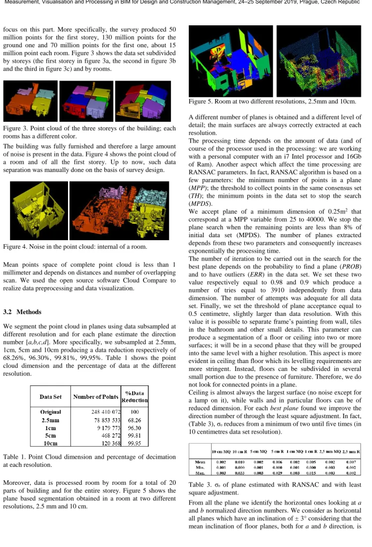
As well known, RANSAC extracts first the principal planar surfaces contained in the data set. Moreover, because of the small threshold used (±0.5cm) the same surface can be segmented in more than one plane. In each data set, among the horizontal planes, the ceiling and floor are extracted. Figure 7 shows the subdivision of a surface in more planes. The elaboration is obtained at a resolution of 1 centimetre; the number of points for each plane varies depending on the resolution. Figure 7 (a) shows the ceiling of the room divided into 5 planes: the red composed of about 95000 points, the blue about 20.000 points, the yellow 7500 points, the green 3500 points and the orange 3000 points. Figure 7 (b) shows the floor

of the balcony divided into 3 planes: the red one, the largest has about 30000 points. Figure 7 (c) illustrate a floor divided into 3 planes: the red one has about 45,000 points.

Figure 7. (a) A ceiling of a room, (b) a floor of a balcony, (c) a floor of a room.

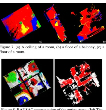
Figure 8. RANSAC segmentation of the entire storey (left The

ceiling and right the floor).

It is evident that floor planes (figure 7b and figure 7c) have a minor segmentation than ceiling planes (figure 7a). Moreover, floors are more horizontal compared with ceilings, this is justified by its horizontality requirement that is more stringent than that of ceilings. The same behavior is evident in Figure 8 which shows the segmentation of an entire storey (the second one). Figure 8(a) shows the ceiling with its segmentation in several planes (one color for each plane), while Figure 8 (b) shows the floor with a single major plane, the red one, composed of about 100000 points. All the others (the white points), subdivided among more minor planes, are about 15000 points. Besides, ceilings are less noisy than floors, as rooms are usually furnished. This characteristic is taken into account in other study (Armeni et al., 2016, Bassier et al., 2016).

4.2 Results of the different resolutions

The standard deviation of the direction number (a,b,c) obtained at the 4 different resolutions is 0.007 m. Moreover, the height of the plane, corresponding to parameter d, has a standard deviation of 0.075 m.

Table 4 shows the values of direction numbers (parameters a, b, c, and d) of the ceiling shown in Figure 6 (a) at the different resolutions and the number of points of the largest plane. In this case, the standard deviation of parameter d is 0.0063 m.

Table 4. Variation of the plane parameters at resolution of 10cm, 5cm, 1cm and 2.5mm for second floor.

All the points of the original point cloud are classified as belonging to a selected plane or not if their distance is less than 3 cm.

(5)

Figure 9. Distance of original points from a plane estimated at the 4 different resolution: (a) 2.5 mm; (b) 1 cm; (c) 5 cm; (d) 10 cm.

Figure 9 shows the distance of original points from a plane estimated at 4 different resolutions. The mean distance ranges between ±1 cm in all four. The plane has a slightly different inclination in a corner (pink points) which is evident in all the resolutions. In fact, through RANSAC, the corner results segmented in a different plane in Figure 7(a) (blue plane). Table 5 summarizes the σ0 and the number of points of the original

cloud within a range of ± 3 cm from the plane obtained at the 4 different resolutions. The estimation improves slightly as the resolution increases. It is important to underline that the processing time of data corresponding to the first resolution (2.5mm) is about hundred times more than the last one (10 cm)

Table 5. Points extracted from original data and σ0.

Ceilings and floors are detected from the analysis of the largest consensus set (Figure 6) by means of peak detection through a gradient operation.

Figure 10 shows the horizontal planes identified in the first storey. Red points belong to horizontal planes of the ceiling, while the blue ones to the floor. All the points in green which belong to intermediate horizontal planes are discarded. Yellow points correspond to the staircase landing. This is not considered as a ceiling because of the small number of points.

Figure 10. Plane selected for first level; (a) longitudinal section; (b) axonometric view.

4.3 From rooms to storey

The floor and ceiling levels obtained at each resolution and for each room is summarized in the following figures. Each figure shows floors and ceilings of a storey. Figure 11 and 12 respectively the floor and ceiling of the first storey, figure 13 and 14 of the second storey and figure 15 and 16 of the third storey. Moreover, the value obtained processing data of a single storey (black line in figures) is compared with those derived from each single room. More specifically, red represents the results obtained with a 10cm resolution, blue 5cm, yellow 1 cm and green 2,5mm. Number in abscissa indicate the rooms, while in ordinate the d values are represented.

Figure 11. Floor of first level.

Figure 12. Ceiling of first level.

Figure 13. Floor of second level.

(6)

Figure 14. Ceiling of second level.

Figure 15. Floor of third level.

Figure 16. Ceiling of third level.

Results obtained at the four resolutions agree in the order of millimeter (standard deviation of 4mm) for floors and in the order of centimeter (1.2 cm) for ceilings. This is caused by the larger segmentation of the ceilings in different planes produced by their lower horizontality. Figure 11 shows two different level for the four rooms, which have a height difference of 20 cm.

4.4 Extraction of main level

To date, the floor and ceiling height is calculated as the mean value of all rooms of the storey. Table 6 summarizes the results.

Table 6. Reference value for each main storey of the building. Using the mean value among all the rooms of a storey as reference height for the floors or the ceilings does not take in

account height differences present within a storey. For instance, the room 7 of third storey is a balcony and has a level 20 cm lower than the floor. Another example is the two levels present at the first storey floor, room 2 and 4 are separated from the other two by a step.

The height of the storeys is 2.09 meters for the first, 2.65 meters for the second and 2.57 meters for the third. Furthermore, from the difference between the level of the floor and that of the ceiling of the downstairs storey the floor slab height of third and second levels are calculated, that is respectively 0.22-0.25m (Table 7).

Table 7. Height of level and slab of the building.

Figure 17 shows for each room the difference between its estimated value and that assumed as reference for the storey. Each color represents a distance: blue -3 cm; azure -2 cm and light blue -1 cm; white zero differences; green 1 cm; yellow 2 cm; orange 3 cm and red more than 4 cm; purple more than -4 cm. In grey the rooms not analyzed (stairwell).

5. CONCLUSION

The goal of the present study is the recognition of the main levels of a building from its 3D scan. The presented data set is a point cloud of a three-storey building composed of respectively 4, 8 and 8 rooms. Horizontal planes are extracted with the RANSAC algorithm. A least square method improves the plane estimation by a factor of three. A fast solution is used which is more convenient when dealing with a large number of points for planes such as here. At times there are several millions of points in a plane.

Figure 17. Distance from original point cloud to the estimated planes.

Ceilings are less noisy then floors which are characterized by the presence of furniture. In spite of this, floors are estimated with greater accuracy since their horizontality requirements are more stringent than those of ceilings.

Results obtained at different resolutions have a deviation of ±1cm (except for 2 rooms). Data resolution of 1 cm is a good compromise between processing time and plane description to consider for future elaborations.

(7)

The processing of the entire storey does not permit to detect height differences within a storey, for instance in presence of a step.

Future development of this research will provide a more detailed analyse of the determination of mean value of single room to detect situation like those of the floor of room 7 of the third storey. Moreover, there are construction elements such as stairs which require more accurate analysses.

We would like to conclude by pointing out that the building under examination, located in the municipality of Amatrice, has suffered the damage of the earthquake of 2016. The changes in its levels, certainly the inclinations of the plans may have been caused by such events.

ACKNOWLEDGEMENTS

We would like to thank Engineering Studio of Rieti (SCS Progetti s.r.l.s.) for the survey of the building.

REFERENCES

Armeni, I., Sener, O., Zamir, A.R., Jiang, H., Brilakis, I., Fischer, M., Savarese, S., 2016. 3D Semantic Parsing of Large – Scale Indoor Spaces. (http:77buidongparser.stanford.edu/)

As built, Faro: https://www.faro.com/products/ construction-bim-cim / lighthouse-as-built.

Bassier, M., Vergauwen, M., Van Genechten, B., 2016. Automated Semantic labeling of 3D vector Models for Scan- to- BIM. Conference: Annual International Conference on Architecture and Civil Engineering (ACE 2016), doi: 10.5176/2301-394X_ACE16.83

Cloudworx, Leica: https://leica-geosystems.com/products/laser-scanners/software/leica-cloudworx).

Edgewise, Clearedge:

https: //www.clearedge3d.com/products/edgewise.

Fienen M. N., 2005. The three-point problem, vector analysis and extension to the N-point problem. Journal of geoscience education, 53(3), 257–262. DOI:10.5408/1089-9995-53.3.257. Fischler, M.A., Bolles, R.C., 1981. Random sample consensus: A paradigm for model fitting with applications to image analysis and automated cartography, Communications of the ACM, vol 24: pp 381-395, 06/1981.

Gašinec, J., Gašincová, S., Trembeczká, E., 2014. Robust Orthogonal Fitting of PlaneJournal of the Polish Mineral Engineering Society, 2014, January-June.

Lan, J., Tian, Y., Song, W., Fong, S., Su, Z., 2018. A Fast Planner Detection Method in LiDAR Point Clouds Using GPU-based RANSAC. KDD 2018 Workshop on Knowledge Discovery and User Modelling for Smart Cities August 20, 2018 - London, United Kingdom.

Macher, H., Landes T., Grussenmeyer, P., 2016.Validation of point clouds segmentation algorithms through their application

to several case studies for indoor building modelling. The International Archives of the Photogrammetry, Remote Sensing and Spatial Information Sciences, Volume XLI-B5.

Murali, S., Speciale, P., Oswald, M.R., Pollefeys, M., 2017. Indoor Scan2BIM: Building Information Models of House Interiors, IEEE/RSJ International Conference on Intelligent Robots and Systems (IROS), PAGG. 6126-6133.

Pointcab, Pointcab Cloud Software Company: https://www.pointcab-software.com/.

Previtali, M., Díaz-Vilariño, L., Scaioni, M., 2018. Indoor Building Reconstruction from Occluded Point Clouds Using Graph-Cut and Ray-Tracing.

Son, H., Kim, C, Turkan. Y., 2015. Scan-to-BIM - An Overview of the Current State of the Art and a Look Ahead. doi.org/10.22260/ISARC2015/0050.

Subramaniam, N.A., Ponto, K., 2016. Hierarchical Plane Extraction (HPE): An Efficient Method For Extraction Of Planes From Large Pointcloud Datasets doi:

10.13140/2.1.2535.4242, Conference: ACADIA 2014. Tarsha-Kurdi, F., Landes, T., Grussenmeyer, P., 2007. Hough-Transform and Extended RANSAC Algorithms for Automatic Workshop on Laser Scanning 2007 and SilviLaser 2007, Espoo, Finland. XXXVI, pp.407-412.

Thomson, C., and Boehm, J., 2015. Automatic Geometry Generation from Point Clouds for BIM. Remote Sensing. doi:10.3390/rs70911753.

Volk, R., Stengel, J, Schultmann, F., 2014. Review: Building Information Modeling (BIM) for existing buildings – Literature review and future needs. Automation in Construction 38, Elsevier, pagg. 109 - 127.

Wang, X., Xiao, J., Wang, Y., 2016. Research of Plane Extraction Methods Based on Region Growing. International Conference on Virtual Reality and Visualization doi: 10.1109/ICVRV.2016.56.

Yang, M.Y., Foerstner, W., 2010. Plane detection in Point Cloud Data. Technical Report Nr. 1, 2010 Department of Photogrammetry Institute of Geodesy and Geoinformation University of Bonn. Available at http://www.ipb.uni-bonn.de/technicalreports/.

Zucker, S.W., 1976. Region growing: Childhood and adolescence. Computer Graphics & Image Processing, Elsevier, pp. 382-399.