Esmarie Scholtz
Department of Industrial Engineering University of Stellenbosch
Study leader: James Bekker
Final year project presented in partial fulfilment of the requirements for the degree of Industrial Engineering at Stellenbosch University
B. Eng Industrial
To my mother, father and (little) brother. Because
where would I be? – who would I be?
– what would life be?
Declaration
I, the undersigned, hereby declare that the work contained in this final year project is my own original work and that I have not previously in its entirety or in part submitted it at any university for a degree.
. . . .
ECSA Exit Level Outcomes Reference
Outcome Reference
Sections Pages
1. Problem solving: Demonstrate competence to identify, assess, formulate and solve convergent and divergent engineering problems creatively and innovatively.
All All
5. Engineering methods, skills and tools, includ-ing information technology: Demonstrate com-petence to use appropriate engineering methods, skills and tools, including those based on informa-tion technology.
2, 3, 4, 5, 6 & 7 8 – 58
6. Professional and technical communication: Demonstrate competence to communicate effec-tively, both orally and in writing, with engineering audiences and the community at large.
All All
9. Independent learning ability: Demonstrate competence to engage in independent learning through well developed learning skills.
2, 3, 4 & 5 8 – 32
10. Engineering professionalism: Demonstrate critical awareness of the need to act professionally and ethically and to exercise judgment and take responsibility within own limits of competence.
Acknowledgements
I would like to acknowledge Mr. James Bekker for his guidance, encour-agement and the expectations he had of both this final year project and I. I also greatly appreciate and admire Mr. Bekker’s willingness to share his wealth of knowledge. I have to admit that I really hate compiling agendas, but prepared mine for project meetings happily.
Thank you to Delyno du Toit for his willingness to answer those questions he was not contractually bound to avoid.
Thank you also to my friends for their interest, encouragement and support throughout the year. It meant more to me than these two sentences can describe.
Annelie and Stephanie need special mention. Your friendships mean the world to me. The mining and manufacturing meccas of Mpumalanga and the Eastern Cape, respectively, are lucky to have you two as residents in 2012.
To the industrial engineering class of 2011: it was fun hanging in Birga with you! You know some pretty awesome people are involved when the words “fun” and “Birga” are used in the same sentence.
Abstract
Cash management is a multi-objective optimisation problem which aims to maximise the service level provided to customers at minimum cost. The topic ofdu Toit(2011)’s masters thesis was automated teller machice (ATM) cash management for a specific South African retail bank. Focus was placed on an ATM network which primarily provides cash to blue collar laborers in the rural Eastern Cape. The aim of this final year project is to refine the work done by du Toit through the specific investigation into the effect of applying a combination of the vehicle routing problem (VRP) and continu-ous review policy for inventory management to the retail banking industry. A decision support system (DSS) in the form of a stochastic, discrete-event simulation model is developed. 90 different scenarios are experimented with using the DSS. Results show that the application of the VRP consistently yields high service levels at low cost when compared to two other routing ap-proaches: first-in-first-out routing and direct replenishment. It is concluded that use of the VRP is especially beneficial when the bank has substantial control over transportation cost. The principal recommendation is there-fore that cost control should be maximised to fully exploit the advantages obtainable from effective cash management. Finally, it is argued that the benefits to be gained from effective cash management (higher service levels at lower cost) can lead to the improvement of the lives of many a South African wage earner. These benefits could also lead to an increased profit margin – life is all about choices.
Opsomming
Kontantbestuur is multi-doelstelling optimeringsprobleem waarvan die doel-wit is om die diensvlak wat aan kli¨ente gelewer word, te maksimeer, ter-wyl koste minimeer word. Die onderwerp van du Toit (2011) se meesters tesis was outomatiese tellermasjien (OTM) kontantbestuur vir ’n spesifieke Suid-Afrikaanse kleinhandelbank. Fokus is geplaas op ’n OTM netwerk wat hoofsaaklik kontant aan arbeiders in die landelike Oos-Kaap voorsien. Die doel van hierdie finale jaar projek is om du Toit se werk te verfyn deur spe-sifiek ondersoek in te stel na die effek wat die toepassing wat ’n kombinasie van die voertuigskeduleringsprobleem en die deurlopende hersieningsbeleid vir voorraadbestuur sal hˆe. ’n Stogastiese, diskrete-gebeurtenis simulasie model is ontwikkel om as besluitnemings ondersteuningstelsel te dien. 90 verskillende eksperimente is met die simulasie model voltooi. Resultate toon dat die toepassing van die voertuigskeduleringsprobleem deurlopend ho¨e diensvlakke teen vergelykende lae koste tot gevolg het. Die voertu-igskeduleringsprobleem word vergelyk met twee ander skeduleringstegnieke: eerste-in-eerste-uit skedulering en direkte aanvulling. Die gevolgtrekking word gemaak dat gebruik van die voertuigskeduleringsprobleem veral vo-ordelig is wanneer die bank aansienlike beheer oor vervoerkoste het. Die hoof aanbeveling is daarom dat kostebeheer gemaksimeer behoort te word om ten volle munt te slaan uit die voordele wat moontlik gemaak word deur effektiewe kontantbestuur. Ten slotte word daar aangevoer dat die voordele wat sal volg uit effektiewe kontantbestuur (ho¨er diensvlakke teen laer koste), die lewens van vele Suid-Afrikaanse loonwerkers kan verbeter. Di´e voordele kan ook lei tot ’n vergrote winsmarge – die lewe is vol keuses.
Contents
1 Introduction 1
1.1 Problem statement . . . 1
1.2 Research rationale and motivation . . . 4
1.2.1 Delyno du Toit: ATM cash management for a South African retail bank . . . 4
1.2.2 Research rationale and motivation: Refining du Toit’s work . . . 4
1.3 Literature on cash management in the retail banking industry . . . 5
1.3.1 A decision support model for the cash replenishment process in South African retail banking . . . 5
1.3.2 The optimal cash deployment strategy . . . 6
1.4 Project objectives . . . 6
1.5 Research methodology . . . 8
1.6 Structure of the report . . . 8
1.7 Conclusion: Introduction . . . 9
2 Multi-objective optimisation 10 2.1 MOO principles . . . 10
2.2 Simulation as a MOO problem solving tool . . . 11
2.3 Simulation modelling: service level versus total cost . . . 15
2.3.1 Total service level . . . 15
2.3.2 Total cost . . . 15
CONTENTS
3 Inventory management 21
3.1 Inventory management models . . . 21
3.2 Inventory situation in question . . . 22
3.3 Formulation of inventory management model . . . 22
3.4 Conclusion: Inventory management . . . 24
4 Vehicle routing 25 4.1 Existing vehicle routing methods . . . 25
4.1.1 The travelling salesperson problem . . . 26
4.1.2 The vehicle routing problem . . . 26
4.1.3 Vehicle routing applications in open literature . . . 27
4.2 Vehicle routing situation . . . 29
4.3 Suggested vehicle routing model . . . 30
4.4 Solving vehicle routing problems . . . 32
4.5 Conclusion: Vehicle routing . . . 32
5 An algorithm for dispensing denominations 33 5.1 Dispensing denominations . . . 33
5.2 The knapsack problem . . . 34
5.3 Suggested algorithm for denomination dispensing . . . 35
5.4 A numerical example of the denomination dispensing algorithm . . . 36
5.5 Algorithms for solving integer programming problems . . . 37
5.6 Conclusion: An algorithm for dispensing denominations . . . 37
6 Simulation study 38 6.1 The simulation model developed for the final year project . . . 38
6.2 A decision support model for vehicle routing in the retail banking industry 39 6.3 Controlled variables . . . 40
6.3.1 Routing method . . . 40
6.3.2 Number of vehicles . . . 41
6.3.3 Routing point . . . 41
6.3.4 Minimum number of ATMs on a route . . . 41
6.3.5 Reorder point . . . 42
CONTENTS
6.4 Uncontrolled variables . . . 43
6.5 Simulation study experiments . . . 43
6.6 Conclusion: Simulation study . . . 46
7 Analysis of simulation study results 47 7.1 The effect of the cost structure . . . 48
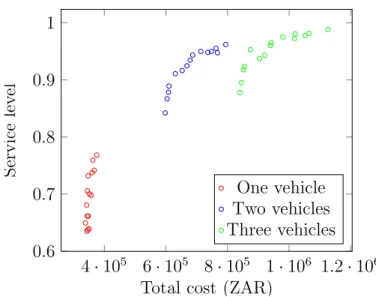
7.2 Varying the number of vehicles . . . 49
7.2.1 Varying the number of vehicles: Status quo cost structure . . . . 49
7.2.2 Varying the number of vehicles: Adjusted cost structure . . . 50
7.2.3 Varying the number of vehicles: General observations . . . 51
7.3 Varying the routing method . . . 53
7.3.1 Varying the routing method: Status quo cost structure . . . 53
7.3.2 Varying the routing method: Adjusted cost structure . . . 54
7.3.3 Varying the routing method: General observations . . . 55
7.4 Varying the routing point . . . 56
7.4.1 Varying the routing point: Status quo cost structure . . . 56
7.4.2 Varying the routing point: Adjusted cost structure . . . 57
7.4.3 Varying the routing point: General observations . . . 58
7.5 Varying the reorder point . . . 59
7.5.1 Varying the reorder point: Status quo cost structure . . . 59
7.5.2 Varying the reorder point: Adjusted cost structure . . . 59
7.5.3 Varying the reorder point: General observations . . . 59
7.6 Summary of global observations . . . 61
7.7 Conclusion: Analysis of results . . . 62
8 Summary and conclusions 63 8.1 Project summary . . . 63
8.2 Recommended cash management strategy . . . 64
8.3 How this final year project benefits society . . . 66
8.4 What the student learned . . . 66
CONTENTS
A Model conceptualisation and translation 68
A.1 Introduction: Functional specification . . . 68
A.2 The functional specification . . . 69
A.2.1 Equipment . . . 69
A.2.2 Product types . . . 70
A.2.3 Operations . . . 71
A.2.4 Transport . . . 71
A.2.5 Input data . . . 71
A.2.6 Output data . . . 73
B Simulation model implementation 74 B.1 An algorithm for dispensing notes . . . 74
B.2 Vehicle routing . . . 76
B.2.1 Near shortest path routing . . . 76
B.2.2 First-in-first-out routing . . . 81
B.2.3 Direct replenishment . . . 81
C Simulation model verification and validation 84
D Results of the simulation study 86
E Delyno du Toit: Meeting agenda and minutes 109
F Documentation of meetings with study leader 111
G Project plan 122
List of Figures
1.1 A graphic illustration of the essence of the research problem. . . 3
1.2 A graphic illustration of the decision support model to be delivered. . . 7
2.1 Steps in a simulation study. . . 13
2.2 Simulation as a MOO decision support system. . . 14
2.3 MOO mapping. . . 14
2.4 Logistics cost breakdown. . . 17
2.5 Logistics cost breakdown adjusted for ATM network model. . . 18
3.1 Some characteristics of the (s, S) inventory management process. . . 23
3.2 The (s, S) inventory management process to be implemented. . . 23
7.1 Overall difference between status quo and adjusted cost structures. . . . 49
7.2 Effect of number of vehicles available: Status quo cost structure. . . 50
7.3 Effect of number of vehicles available: Adjusted cost structure. . . 51
7.4 Overall effect of the number of vehicles available. . . 52
7.5 Effect of routing method: Status quo cost structure. . . 54
7.6 Effect of routing method: Adjusted cost structure. . . 55
7.7 Overall effect of routing method. . . 56
7.8 Effect of the routing point: Status quo cost structure. . . 57
7.9 Effect of the routing point: Adjusted cost structure. . . 58
7.10 Overall effect of the routing point. . . 59
7.11 Effect of the reorder point: Status quo. . . 60
7.12 Effect of the reorder point: Adjusted cost structure. . . 60
LIST OF FIGURES
8.1 The set of Pareto optimal solutions for the MOOP. . . 65
E.1 Agenda and minutes for meeting held with Delyno du Toit. . . 110
F.1 Page one of agenda and minutes for meeting on 4 March 2011. . . 112
F.2 Page two of agenda and minutes for meeting on 4 March 2011. . . 113
F.3 Time sheet for meeting on 4 March 2011. . . 114
F.4 Page one of agenda and minutes for meeting on 15 August 2011. . . 115
F.5 Page two of agenda and minutes for meeting on 15 August 2011. . . 116
F.6 Time sheet for meeting on 15 August 2011. . . 117
F.7 Page one of the supplement to the agenda for meeting on 15 August 2011.118 F.8 Page two of the supplement to the agenda for meeting on 15 August 2011.119 F.9 Page three of the supplement to the agenda for meeting on 15 August 2011. . . 120
F.10 Page four of the supplement to the agenda for meeting on 15 August 2011.121 G.1 Project plan for the final year project. . . 123
List of Tables
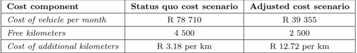
6.1 Status quo cost structure compared to additional adjusted cost structure. 43
6.2 Simulation model experiments with status quo cost structure. . . 44
6.3 Simulation model experiments with adjusted cost structure. . . 45
8.1 Scenarios resulting in lowest cost, highest service level and a good com-promise. . . 65
A.1 ATM cash management: Operational and cost details. . . 70
Nomenclature
Acronyms
ATM Automated teller machine.
BKP Bounded knapsack problem.
CIT Cash-in-transit.
CVRP Capacitated vehicle routing problem.
DCVRP Distance-constrained capacitated vehicle routing
prob-lem.
DP Dynamic programming.
DVRP Distance-constrained vehicle routing problem.
EOD End of day.
EOM End of month.
FIFO First-in-first-out.
IP Integer programming problem.
KP Knapsack problem.
LP Linear programming problem.
MCDM Multiple criteria decision making.
Nomenclature
MOO Multi-objective optimisation.
MOOP Multi-objective optimisation problem.
NSP Near shortest path.
OTM Outomatiese tellermasjien (Afrikaans for ATM).
TSP Travelling salesperson problem.
VRPB Vehicle routing problem with backhauls.
VRPPD Vehicle routing problem with pickup and delivery.
VRPTW Vehicle routing problem with time windows.
VRP Vehicle routing problem.
Greek Symbols
e Euler’s number.
Roman Symbols
CC Total capacity cost.
ckm Cost per kilometer.
qi Delivery size.
pi Denomination value.
dij Distance between stationsiand j.
CD Total distance cost.
Di Distance covered by vehicleiin a month.
CDi Distance cost per vehicle.
re Effective daily interest rate.
Nomenclature
bj Number of identical copies of item typej available.
uj Variable indicating the number of alternativeiincluded
in the solution.
xij Integer variable denoting the number of times an arcdij
is traversed by the optimal solution.
Ir Cash on hand at time of replenishment.
Ij Cash level at the end of day j.
G Item set for the knapsack problem.
AK Capacity value of the knapsack.
SAT M Subset of the station set including ATMs that are
tra-versed by the optimal solution.
k(SAT M) Minimum number of vehicles required to serve al
cus-tomers in vertex setSAT M ⊆V.
fi(x) Set of objective functions of a MOOP.
SM OO MOO solution space.
rn Nominal annual interest rate.
nAT M Number of ATMs.
nK Number of items with profitpj and weight wj available
for ‘filling’ the knapsack.
m Number of months in the cost calculation period.
yi Number of notes of denomination valuepi.
nM OO Number of MOO objective functions.
nT SP Number of points covered by the TSP.
Nomenclature
K Number of vehicles.
x nM OO-vector of decision variables.
CO Opportunity cost.
pj Profit of knapsack item.
CR Total rebanking cost accrued.
cR Rebanking cost per R 100.
s Reorder point when using the (s, S) policy for inventory
management.
S Reorder quantity when using the (s, S) policy for
inven-tory management.
Tr Time required to replenish one ATM.
Zi Set of objective function values serving as the solution
space for a MOOP.
Troute Time required to complete a determined route.
Xi Set of scenarios decided upon for the simulation study.
V The station set.
AV Delivery vehicle capacity.
CV Monthly cost associated with using one CIT vehicle.
v Vehicle speed measured in kilometers per hour.
wj Weight of knapsack item.
Terminology
Cash out Any event where the cash level in an ATM is such that customer demand cannot be met.
Nomenclature
Direct replenishment Routing method where vehicles are dispatched directly to ATMs as ATMs register orders.
Even-note-picking Denomination dispensing algorithm used in industry. Notes are picked in a way which evens out inventory levels of the different notes available.
Least-note-picking Denomination dispensing algorithm used in industry. Notes are picked in a way which minimises the number of notes dispensed.
Near shortest path routing Routing method where the aim is to minimise the dis-tance vehicles travel using the VRP.
Pareto principle Principle stating that 20% of causes are responsible for 80% of effects.
Replenishment efficiency Number of ATMs replenished using a single route. Also referred to as routing efficiency.
Routing efficiency Number of ATMs replenished using a single route. Also referred to as replenishment efficiency.
Routing point Minimum number of ATMs that need to have registered an order before a route will be determined.
Service level The proportion of the total number of customers satis-factorily served to the total number of customers requir-ing service.
Speed of service Time elapsed between the moment an ATM registers an order and its replenishment.
(s, S) policy Inventory management policy where srefers to the re-order level andS to the reorder quantity.
Chapter 1
Introduction
The aim of this final year project is to apply engineering methods, skills and tools to refine work done bydu Toit(2011) on the determination of the optimal cash deployment strategy for a South African retail bank. More specifically, a combination of operations research techniques will be used to develop a decision support system which will aid decision making regarding this multi-objective optimisation problem. This chapter will set out the problem statement and provide documentation of the literature study done on work relating to du Toit (2011)’s thesis. The project objectives and methodology will be laid out. Finally, the structure of the report will be detailed.
1.1
Problem statement
ATMs (automated teller machines) form a key part of retail banking service provision. For many clients ATM withdrawals are the only way to obtain the cash necessary for everyday living. If an ATM is out of cash, these clients face a predicament.
“Out of cash” might refer to an ATM that has absolutely no cash left, but the term may also refer to an ATM that has run out of certain denominations and can therefore not provide a specific amount. An ATM that has run out of R 50 notes, for example, would be unable to dispense multiples of R 50. If a specific ATM or the ATMs operated by a particular bank, is out of cash (or is unable to dispense the exact amount required by the client) on a regular basis, a real possibility exists that customers would switch to a bank better able to meet their cash requirements.
1.1 Problem statement
It is thus important, from the perspective of a consumer bank, to ensure that cash levels within its ATMs are sufficient for as large a proportion of time as possible. For now, let the ’proportion of time an ATM is not out of cash’ be the service level of an ATM. To provide the highest possible service level to customers, it is necessary to have some cash in an ATM, but preferable that all the denominations are in stock, at all times.
Providing a 100% service level for one ATM would be simple enough. However, no bank has only one ATM and providing very a high service level to an entire network of ATMs is far more complicated.
An ATM network consists of a number of ATMs (the ATM network in question is made up of 18), each with its own stochastic, seasonal customer demand profile, and a count house from where ATMs are replenished. Several cash-in-transit (CIT) vehicles service a network at costs negotiated with the CIT company. The cost structure negotiated and the resulting cost to the bank are dependent on the total distance covered by CIT vehicles.
The ATM network at hand is situated in the rural Eastern Cape. Distances between these ATMs are great (see Table A.2 in Appendix A) and the costs associated with covering these distances can therefore be significant. This was the reason for researching this specific ATM network.
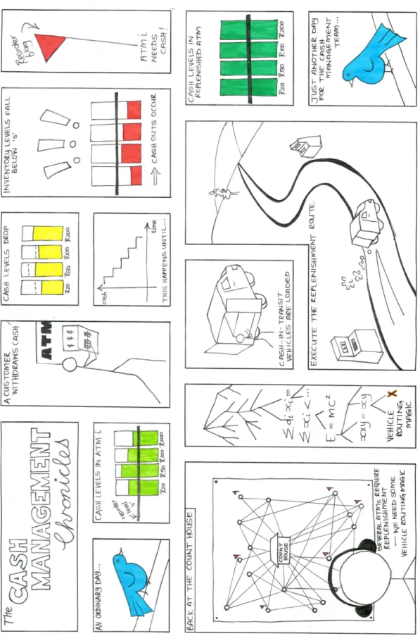
Figure 1.1 (the student’s handiwork) illustrates the essence of the problem in a simple, lighthearted fashion. Note the rolling hills of the countryside in which the ATM network is located.
Due to fact that retail banks have full control over inventory levels in ATMs (un-like, for example, a soft drink distributor delivering stock to outlets controlling their own inventory levels), providing 100% service levels to an entire ATM network would be ambitious, but achievable if the transportation and inventory costs of having all denominations in stock at all times could be ignored. Costs associated with delivery delays, transportation and inventory (amongst other ATM operating costs) are, how-ever, very real and cannot be disregarded. Cash transit costs involve not only fuel and labour but also rigorous security and high risk. To a bank, cash in an ATM is not earning interest and is therefore adding to existing inventory costs. In the competitive consumer banking industry, unreasonably high costs – such as the costs associated with maintaining a perfect service level for an ATM network – are unaffordable.
1.1 Problem statement
1.2 Research rationale and motivation
Taking these costs into account, the problem is thus: how can the service level of the researched ATM network, operated by the particular bank, be maximised at minimum cost using industrial engineering techniques?
1.2
Research rationale and motivation
The problem stated above is a simplification of a problem researched bydu Toit(2011). His work forms the basis for this project and will now be discussed, after which details on the research rationale and motivation will be provided.
1.2.1 Delyno du Toit: ATM cash management for a South African retail bank
“ATM cash management for a South African retail bank”, du Toit (2011)’s thesis, resulted from his career at a South African retail bank. The cash management strategy in du Toit’s thesis is developed for a network of ATMs operated by the retail bank. The network is located in the Eastern Cape and consists of 18 ATMs and one count house. A cash-in-transit security company handles cash distribution in the region. At the time the thesis was written the cash management strategy used by the bank relied heavily on experience and personal judgement.
As a result, the thesis focuses primarily on prediction methods and inventory man-agement models. Secondary focus is placed on routing techniques found in the op-erations research field; du Toit only investigated the travelling salesperson problem , comparing it to direct replenishment. Simulation is used to compare different inventory management models, routing techniques and combinations thereof.
Du Toit concludes that these techniques could achieve significant savings in the retail banking environment. The Holt-Winters prediction method and the TSP for vehicle routing are recommended. Du Toit does not make definite conclusions about the inventory models investigated and suggests further research in these areas.
1.2.2 Research rationale and motivation: Refining du Toit’s work Delyno du Toit completed his masters thesis for graduation in March 2011 with the study leader. The main focus of his work was to determine if the application of indus-trial engineering techniques to the retail banking would lead to significant cost savings.
1.3 Literature on cash management in the retail banking industry
He focused mainly on demand forecasting with little attention paid to vehicle routing and inventory management.
The study leader was not convinced that du Toit’s work provided satisfactory in-dication of the effects of vehicle routing and inventory management as components of a cash management strategy. In order to refine the work done by du Toit, the study leader specifically required that attention be paid to the application of the vehicle routing problem (instead of the TSP) and the continuous review policy for inventory management. It was specified that the refinement must be done using discrete-event simulation. The work done to refine du Toit’s work must follow a multi-objective optimisation (MOO) approach as the stated problem is a MOO problem.
1.3
Literature on cash management in the retail banking
industry
Due to the high importance of security in the banking industry, it is difficult to find related work in the open literature. The student had access todu Toit (2011)’s work (with the clear instruction to “not leave it lying around”) due to the fact that this final year project serves as a refinement of the work done in it. There are two other works openly available, which are discussed below.
1.3.1 A decision support model for the cash replenishment process in South African retail banking
The first application of industrial engineering techniques in the South African retail banking environment document in the open literature is attributed toAdendorff(1999). Having investigated a South African retail bank branch for three months, Adendorff determined the nature of the demand distribution. From there an appropriate forecast-ing model was developed. After evaluatforecast-ing the existforecast-ing order policies of the branch, a decision support model for the improvement of the cash replenishment process was developed.
Adendorff concludes that significant savings can be achieved through the application of industrial engineering techniques in the retail banking industry.
1.4 Project objectives
The focus Adendorff places on factors defining the South African retail banking environment, such as the crime situation, are worth noting.
1.3.2 The optimal cash deployment strategy
Wagner (2007) develops a conceptual framework for finding the optimal cash deploy-ment strategy for a network of ATMs. For the purpose of the thesis, ‘optimal’ is equivalent to ‘minimum-cost’. In determining a minimum-cost scheduling and replen-ishment strategy, logistics costs (holding cost plus the cost of rent), inventory policies and replenishment vehicle routing are taken into account.
Conceptually, Wagner assumes the existence of a perfect forecasting model, effec-tively eliminating the actual stochastic nature of demand. Focus is placed on the development of primarily deterministic scientific and simulation models.
Due to the algorithmic complexity of the inventory routing problem applied to a network of ATMs, confirmation about the effects of its application could not be given. The combined use of the Wagner-Whitin algorithm as inventory policy and the travelling salesperson problem for vehicle routing yielded the best result. Wagner concludes that substantial cost savings can be achieved using optimisation.
The work done by Wagner has focus similar to that of this project. There are, however, significant differences: firstly, the final year project is a MOO problem aiming to maximise service level, whilst minimising cost. Furthermore, it will aim to account for stochastic, seasonal demand, true the real-world situation. The effect of using the vehicle routing problem (VRP) instead of the TSP will also be investigated.
1.4
Project objectives
The primary objective of the final year project is to refine the work done by du Toit
(2011). This refinement must at least achieve the following secondary objectives:
1. Provide an indication of the effect of applying the VRP to the retail banking industry.
• None of the work discussed thus far applied the VRP. The reader will note in Chapter4 that none of the literature available on the VRP applies it to retail banking. This is ground breaking stuff. Are you excited?
1.4 Project objectives
2. Supply a clear indication on how the continuous review policy should be applied for inventory management.
3. Deliver a decision support model with which a MOO set of solutions can be determined.
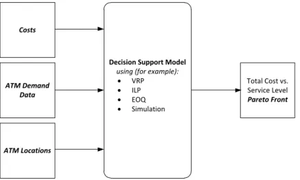
Figure 1.2 (as demonstrated by Bekker (2011a)) illustrates how such a decision support model functions.
Decision Support Model
using (for example): · VRP · ILP · EOQ · Simulation Costs ATM Demand Data ATM Locations Total Cost vs. Service Level Pareto Front
Figure 1.2: A graphic illustration of the decision support model to be delivered.
The three secondary objectives are compulsory refinements. The student was free to identify and make additional refinements. A discussion on additional refinements that were decided upon follows.
Wagner(2007) anddu Toit(2011) both used simulation modelling. All indications are that both ignored some details associated with dispensing cash: the inventory level in an ATM does not simply drop R 250 when a customer demands R 250, but the number of R 200 and R 50 notes that are available becomes less. Wagner (2007) worked with the total number of banknotes withdrawn over a period, whereasdu Toit
(2011) used total daily withdrawal amounts.
The student argues that the fact that meeting customer demand requires the avail-ability of a specific combination of notes for every withdrawal event must be taken into account. To do so, an algorithm must be determined according to which the cash amount demanded by a customer is made up.
1.5 Research methodology
As the final year project progressed, the student decided to do an elementary sen-sitivity analysis on the cost structure of the problem. This is an additional refinement ondu Toit (2011)’s work.
1.5
Research methodology
To reach primary and secondary project objectives, a certain approach must be followed. The approach used is dictated in part by the research rationale. The methodology followed comprises of five main phases:
1. Do a literature study on related work available to gain a full understanding of the problem (as documented in Sections1.3.1and1.3.2).
2. Do a literature study on techniques and methods required to solve the problem: MOO, discrete-event simulation, the VRP, inventory management and integer programming.
3. Develop a simulation model allowing for decision making regarding the VRP and continuous review policy. Such a model should be able to compare different routing approaches for a network of ATMs with stochastic, seasonal demand. Setting up different continuous review policy scenarios should also be possible. Finally, the simulation model should dispense notes according to the algorithm developed by the student. This requires the incorporation of various operations research and programming techniques (as discussed in the chapters to follow). 4. Set up experiments which will illustrate the effects of the VRP and continuous
review policy on the system.
5. Analyse simulation experiment results and draw conclusions about the systems and the variables that affect it.
The section that follows shows that these phases form the backbone of this report.
1.6
Structure of the report
1.7 Conclusion: Introduction
In Chapter 3 emphasis will fall on inventory management: existing models, the current inventory situation and the suggested inventory model will be discussed.
Vehicle routing techniques found in the field of operations research will be the focus of Chapter 4 where the VRP will be concisely compared to the TSP. The suggested vehicle routing model will be formulated.
Chapter 5 will show the development of an algorithm with which notes can be dispensed to meet customer demand.
An overview of the experiments drawn up for the simulation study will be given in Chapter6.
The results of said simulation study will be analysed and discussed in Chapter 7. Chapter 8will serve as summary and conclusion to the final year project report.
1.7
Conclusion: Introduction
This chapter stated the MOO problem to be addressed by the final year project: max-imising the service level of an ATM network at minimum cost. It was emphasised that the project serves as a refinement of work done by du Toit (2011). “ATM cash management for a South African retail bank” was therefore reviewed as part of the research rationale and motivation. Next, literature regarding cash management in the retail banking industry was outlined. The primary and secondary project objectives were identified and the research methodology was subsequently discussed. Finally, the structure of the report was laid out. Chapter 2 will provide information on MOO and discrete-event simulation as a MOO problem solving tool. The two project objective functions will be defined and detailed.
Chapter 2
Multi-objective optimisation
The previous chapter was the introduction to the final year project report. It stated the problem, laid out the research rationale and motivation, and reviewed literature on cash management. The project objectives were introduced and the research method-ology developed. This chapter will provide information about basic multi-objective optimisation concepts. Discrete-event modelling will be discussed as it can be seen as a MOO problem solving tool. Finally, the two objective functions for the project are broken down.
2.1
MOO principles
As stated in Section 1.1, the question to be answered in this project is: how can the service level of an ATM network be maximised at minimum cost. Two conflicting objectives must thus be considered. This is usually the case when it is impossible to tie all decision making criteria into a single trade-off function (Zeleny,1974). Problems of this nature are referred to as multi-objective optimisation (MOO) problems, multiple criteria decision making (MCDM) problems (Thieleet al.,2009) or vector optimisation problems (Ravindran,2008), to name a few.
Optimal solutions to individual objectives of the MOO problem (MOOP) do not occur at the same alternative (Ravindran,2008). The aim of solving a MOO problem is therefore not to find the optimal solution (as it does not exist) but rather a set of solutions where all objectives are at their “best” possible values under the given con-ditions (Zeleny,1974). Such a set is referred to as efficient, nondominated, noninferior
2.2 Simulation as a MOO problem solving tool
or Pareto optimal solutions (Thiele et al., 2009). If x denotes an n-vector of decision variables andfi(x), i= 1, . . . , krepresents thekobjective functions of a MOOP,
Ravin-dran(2008) describes the Pareto optimal set of solutions as: “A solutionx◦∈SM OO to
a MCDM problem is said to be efficient if fk(x)> fk(x◦) for some x∈SM OO implies
thatfi(x)< fi(x◦) for at least one other indexi.”
2.2
Simulation as a MOO problem solving tool
Simulation provides a method of analysing real-world systems using software designed to imitate system characteristics. It is most applicable when studying complex systems (Kelton et al.,2004). Simulation aids decision making, improves stake holders’ under-standing of the system and allows decision makers to explore possibilities. It can also help in diagnosing problems, identifying constraints and specifying system requirements (Banks et al.,1998).
Keltonet al.(2010) provides an introduction to basic simulation concepts. The book distinguishes between static and dynamic simulation models, continuous-change versus discrete-change dynamic models and differentiates between deterministic and stochas-tic simulation models. Focus falls on dynamic, discrete-change, stochasstochas-tic simulation models built using the Simio software package.
For more information on simulation, the reader is referred to Kelton et al.(2004),
Keltonet al. (2010) and Bankset al. (1998).
Dynamic, discrete-change, stochastic simulation will be used for the problem at hand. The problem is ‘dynamic’ because the system changes with time. Even though the system changes with time, it does not change continuously but rather due to the occurrence of specific events, thus: ‘discrete-change’. Finally, inputs in the simulation model are not certain, but stochastic. On the recommendation of the study leader Arena is used for building the simulation model. Keltonet al. (2004) introduces simu-lation concepts, focusing on modelling dynamic, discrete-change, stochastic systems in Arena. The Arena work package, operations modelling and statistical considerations are detailed.
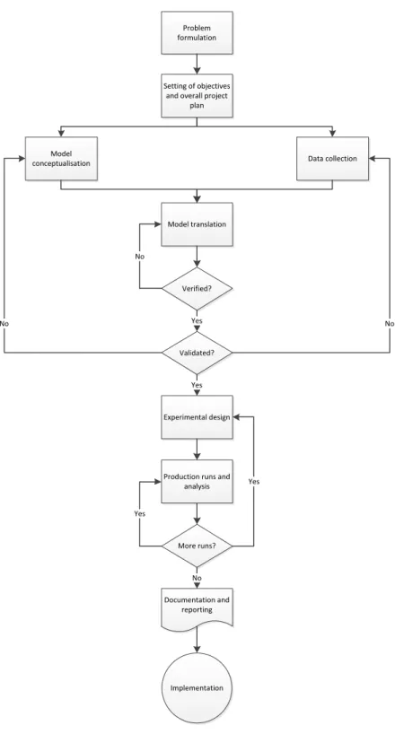
Banks et al. (1998) suggest the simulation process illustrated in Figure 2.1. The steps in a simulation study correspond well with the execution of the final year project. The relationship between the simulation process and the project (and the resulting
2.2 Simulation as a MOO problem solving tool
project report) will now be discussed. A simulation study starts with the formulation of the problem, after which project objectives are decided upon. Chapter 1 contains the problem statement as well as primary and secondary project objectives. Model con-ceptualisation is the process of mathematically formulating the model and is detailed in below as well as in Chapters3, 4and 5. The thesis written bydu Toit (2011) (dis-cussed in Chapter1) along with the data he used for writing it make up a part of ‘Data Collection’. A personal interview with him as well as questions asked and answered via email correspondence make up a further part of ‘Data Collection’. Details on the conceptualisation (not contained in Chapters3,4 and5) and translation of the model can be found in Appendices A and B. Model verification was done throughout model implementation and translation. The validation of the simulation model is discussed in AppendixC.
Once a working model exists, experiments can be designed and run. The experimen-tal design is discussed in Chapter6. Chapter6 also provides introductory information on the production runs. As was mentioned in Chapter 1, the results of the 45 initial experiments led to an additional cost structure being drawn up. 45 more experiments were run using the adjusted cost structure. The answer to the “More runs?” question asked by Banks et al. (1998), was thus “Yes”. Finally Banks et al. (1998) suggest that the model be documented thoroughly after which the results can be reported (re-sults are discussed in Chapter 7). This report serves as partial documentation of the model; meeting agendas, minutes and explanatory notes serve as further documenta-tion. Comments accompanying programming code (written in VBA for Arena) are a further addition to the model documentation. The implementation step can be ignored for the purposes of this project, but the results will be discussed with representatives of the retail bank for their interest. If deemed fit to do so, the retail bank can then implement the suggestions made by the student or changes of their own based on the results of the simulation study.
The ATM network in question is nothing if not a complex system. For seasonally variable demand unique to the ATM, the machine dispenses denominations according to a specified algorithm. Depending on the inventory level in an ATM, stock might have to be added. This applies to the entire network of ATMs. Given that some ATMs require replenishment and others not, an optimal vehicle routing needs to be
deter-2.2 Simulation as a MOO problem solving tool
Problem formulation
Setting of objectives and overall project
plan
Model translation
Production runs and analysis Experimental design Data collection Model conceptualisation Verified? Validated? More runs? Documentation and reporting Implementation No Yes No No Yes No Yes Yes
2.2 Simulation as a MOO problem solving tool
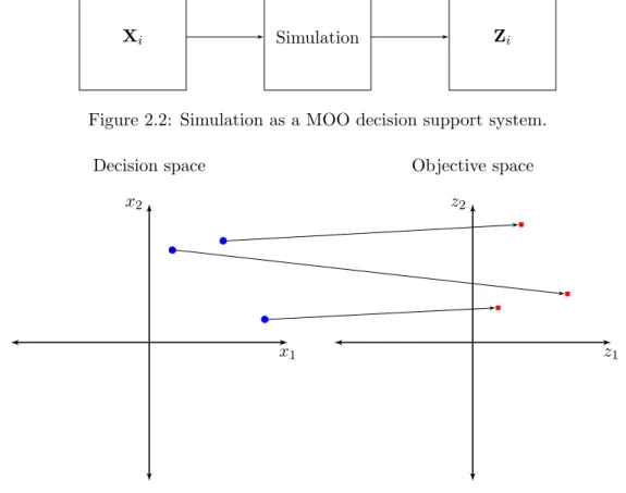
Xi Simulation Zi
Figure 2.2: Simulation as a MOO decision support system.
x1
x2
z1
z2
Decision space Objective space
Figure 2.3: MOO mapping.
mined. Additionally, this is a MOO problem and not only one, but two optimisation objectives need be considered. The problem yields itself very well to simulation.
In essence simulation enables simulation analysts to evaluate the effects of changes in certain variables on the complex system studied. The analyst decides on a set of scenarios (Xi) for the simulation study. These scenarios are combinations of variables
chosen from the decision space and serve as an input to the simulation model. For each scenario, the simulation model yields a unique response. A specific reorder level or routing method would, for example, produce a certain response. These responses make up Zi a set of objective function values serving as the solution space for the MOOP.
From the solution space, a Pareto front containing efficient solutions can be obtained. Figure 2.2shows this process: scenarios serve as input to the simulation model which yields the solution space. Figure 2.3 shows how scenarios chosen for the simulation study map onto the responses produced by the simulation model.
2.3 Simulation modelling: service level versus total cost
2.3
Simulation modelling: service level versus total cost
As stated in Section 1.1, the question to be answered in this project is: how can the service level of an ATM network be maximised at minimum cost. This is a multi-objective optimisation problem with two goal functions: (1) maximise service level and (2) minimise total cost.
Due to the nature of multi-objective optimisation problems, plotting service level against total cost for a large number of experiments should yield a Pareto front. This front represents optimal scenarios. Valuable conclusions about variables affecting the system can be drawn from such a plot and the resulting Pareto front. In order to plot the values of these goal functions, service level and total cost need to be defined. These definitions follow.
2.3.1 Total service level
For this model, acash out will be defined as any situation where a customer cannot be served due to a shortage of cash. An ATM might for example have more than R 70, but in denominations with which a R 70 combination of notes cannot be formed – this would count as a cash out.
Service level for this problem is the ratio of the total number of customers sat-isfactorily served to the total number of customers requiring service. Service level is expressed in Equation2.1.
Service level= Total customers requiring service−Total number of cash outs
Total customers requiring service . (2.1)
From Equation 2.1, the first objective function for the MOOP to be modelled is
maximise Total customers requiring service−Total number of cash outs
Total customers requiring service . (2.2)
2.3.2 Total cost
Costs that need to be considered for the model include cash transportation, handling and storage. These costs are all logistics related expenses.
2.3 Simulation modelling: service level versus total cost
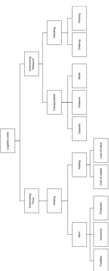
Wagner (2007) recommended work done by Daganzo(2005) as “the most detailed and comprehensive framework for the classification and analysis of logistics costs to date”. Wagner(2007)’s summary ofDaganzo(2005)’s work is shown in Figure 2.4.
Not all the elements taken into account in Daganzo (2005)’s analysis are appli-cable to the current problem. The following elements do not have to be taken into consideration:
• Overcoming “Time” – Holding – Rent: There is no indication in du Toit’s work that the cash in ATMs is insured or protected. The cost associated with renting facilities are not influenced by either the inventory or routing models. • Overcoming “Time” – Waiting – Loss of value: Lost interest will be
con-sidered as ”Cost of capital”.
• Overcoming “Distance” - Transportation - Mode: Only the scenario where dedicated vehicles are used will be considered.
• Overcoming “Distance” – Handling – Ordering: It is assumed that there is no special ordering cost involved with orders from ATMs to the counthouse. Costs involved with ordering are primarily administrative and therefore “fixed” irrespective of the inventory and routing models in use.
Costs which have to be taken into consideration are:
• Overcoming “Time” - Waiting - Cost of capital: Cash kept in ATMs earns no interest. This should be taken into account. A nominal yearly rate of 6% is assumed. For the purposes of this study, the cost of capital will be referred to as “opportunity cost”.
• Overcoming “Distance” - Transportation - Capacity: Increasing capacity (adding an extra vehicle) will impact total cost significantly. A dedicated vehicle costs R 78 710 per month.
• Overcoming “Distance” - Transportation - Distance: The first 4500 km covered by a vehicle in a month is free. After that every kilometer costs R 3.18.
2.3 Simulation modelling: service level versus total cost Lo gi st ic s co st s H ol di ng O ve rc om in g “D is ta nc e” O ve rc om in g “T im e” R en t W ai tin g Fa ci lit ie s In su ra nc e P ro te ct io n C os t o f c ap ita l Lo ss o f v al ue Tr an sp or ta tio n H an dl in g C ap ac ity D is ta nc e M od e O rd er in g P ac ki ng
2.3 Simulation modelling: service level versus total cost Logistics costs Holding Overcoming “Distance” Overcoming “Time” Waiting Cost of capital Transportation Handling
Capacity Distance Packing
Figure 2.5: Logistics cost breakdown adjusted for ATM network model.
• Overcoming “Distance” - Handling - Packing: The only packing cost ap-plicable is that of rebanking which occurs when notes are left in an ATM at the time the ATM is replenished. A rebanking cost of R 0.21 per R 100 rebanked needs to be taken into consideration.
Figure2.5shows a logistics costs breakdown adjusted to suit the project. From this breakdown, the second objective function is
Minimise CO+CC+CD+CR. (2.3)
The opportunity costCOis calculated by multiplying the effective daily interest rate
re with the cash leftIj in an ATM at the end of a day j (du Toit,2011). Opportunity
cost is calculated on a daily basis from the first day of the month until month end
2.3 Simulation modelling: service level versus total cost
monthm. This is shown in Equation 2.4.
CO= m X i=1 EOM X j=1 re×Ij. (2.4)
Equation 2.5 shows the calculation of the effective daily interest rate re for a
con-tinuously compounded annual nominal ratern.
re=ern/365−1. (2.5)
Capacity cost CC is a function of the number of vehicles employed (K) and the
monthly cost associated with using a vehicleCV. m denotes the number of months for
which cost is calculated. Capacity cost is also referred to as “vehicle cost” throughout the project report. The capacity cost denoted by Equation2.6.
CC =
m
X
i=1
K×CV. (2.6)
Furthermore, distance cost CD is the sum of the distance costs per vehicle CDi
with i = 1. . . K. CDi is a function of the distance travelled by each vehicles Di and
dependent onf the number of free kilometers available, andckmthe cost per kilometer.
Distance cost is calculated using Equations2.7 and2.8.
CDi(D) = ( 0 ifDi≤f, (Di−f)×ckm ifDi> f, for i= 1, . . . , K. (2.7) CD(i) = K X i=1 CDi. (2.8)
Finally, rebanking cost CR depends onm the number of ATMs,Ir the cash left in
each ATM at the time of replenishment andcRthe rebanking cost per R 100. Equation 2.9shows the calculation of CR.
CR= nr X r=1 Ir×cR 100 (2.9)
wherenr is the total number of replenishment events that occurred during the cost
2.4 Conclusion: Multi-objective optimisation
2.4
Conclusion: Multi-objective optimisation
This chapter highlighted some important MOO principles, after which simulation was discussed as a MOO problem solving tool. The objective functions for this project – maximise service level; minimise cost – were broken down last.
Chapter 3
Inventory management
The previous chapter focused on multi-objective optimisation and discrete-event simu-lation as a MOO problem solving tool, detailing the simusimu-lation process. The simusimu-lation process starts by identifying the problem and setting project objectives. Once this is done, model conceptualisation can begin. Model conceptualisation begins in Chapter
2where the MOO objective functions for the research project were laid out.
Model conceptualisation continues in this chapter with the discussion of inventory management. As mentioned in Chapter1the refinement that is the aim of this project must at least investigate the effect of the continuous review policy for inventory man-agement. Subsequently this chapter will outline different existing inventory manage-ment models. After which, the inventory situation on hand will be described. Finally, the continuous review policy for inventory management is discussed and the proposed inventory management model is mathematically formulated.
3.1
Inventory management models
Inventory control models can primarily be divided in two categories according to the na-ture of the demand to be met: deterministic inventory models and stochastic inventory models.
Deterministic inventory models deal with certain demand. These models include the economic order quantity formula (EOQ) and Walter-Whitin’s time-varying model (Ravindran,2008).
3.2 Inventory situation in question
Dealing with uncertain demand, stochastic models include the news vendor problem and the (s, S) policy (Winston, 2004). Ravindran (2008) mentions stochastic multi-echelon inventory models. Bellman(1957) discusses a stochastic dynamic programming approach referred to as the “the optimal inventory equation”.
3.2
Inventory situation in question
The inventory situation in the Eastern Cape can be described as a stochastic, multi-echelon system. Inventory levels in the count house can be described as multi-period, whilst inventory levels in ATMs can be managed as either single- or multi-period. Notes can be added to the cash remaining in an ATM during replenishment (this is called a “cash-add” system and would be multi-period management) or the remaining notes can be removed and replaced with newly packed canisters (a single-period inventory management technique referred to as “cash-swap”). Retail banking is a harsh industry and there are no backorders allowed.
The scope of this project does not cover the entire multi-echelon inventory system but focuses only on inventory management of the cash in ATMs, assuming infinite availability of notes at the count house.
3.3
Formulation of inventory management model
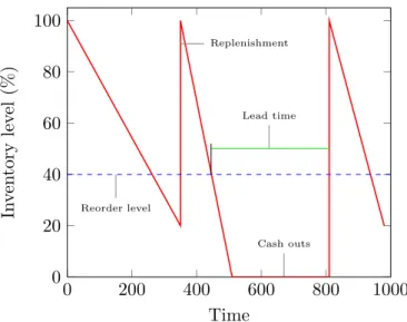
As part of the refinement of du Toit (2011)’s work, various scenarios relating to the continuous review (s, S) policy for inventory management must be investigated. The (s, S) policy involves continuously monitoring stock levels within the ATMs. As soon as the inventory level in ATMidrops below the reorder points, an order is placed which would bring inventory position to S (Axs ˙ater, 2000). Figure 3.1 shows the primary characteristics of the continuous review policy.
The inventory management model developed uses the cash-swap approach described above. Effectively, this means that order size is equal to a fixed S, as the inventory position would become zero when the remaining notes are removed. Once all remaining notes were removed, inventory level increases by said fixedS, bringing inventory levels to 100% every time an ATM is replenished. Figure 3.2 shows the (s, S) policy to be implemented for the simulation model.
3.3 Formulation of inventory management model 0 200 400 600 800 1000 0 20 40 60 80 100 Cash outs Replenishment Reorder level Lead time Time In v en tory lev el
Figure 3.1: Some characteristics of the (s, S) inventory management process.
0 200 400 600 800 1000 0 20 40 60 80 100 Cash outs Replenishment Reorder level Lead time Time In v en tory lev el (%)
3.4 Conclusion: Inventory management
Order sizeS is based on operational data provided bydu Toit(2011): canisters con-taining cash can at most contain 2500 notes. Unfortunately, dispensing problems occur when canisters are filled to the brim. To prevent such errors, newly packed canisters are filled with 2000 notes each. Additionally du Toit(2011) noted that canisters filled with R 200 notes tend to run empty first. For this reason, the retail bank packs two of the five canisters available in an ATM with R 200 notes. Order size can be expressed as S = 4 X i=1 pi×yi (3.1) yi = 2000 fori= 1,2,3, (3.2) y4 = 4000, (3.3) p1 = 20, (3.4) p2 = 50, (3.5) p3 = 100, (3.6) p4 = 200. (3.7)
where yi denotes the number of notes of denomination value pi. The numerical
value of S is R 1 140 000.
For this simulation studySwill not be varied; only changes toswill be investigated. The reorder pointscan be either the total monetary value of cash in the ATM, such as R 300 000, or the total number of notes left in the ATM. The reorder point can also be the number of notes left of a certain denomination: an order could be triggered once there are less than 500 R 50 notes available. The variations insthat were experimented with are discussed in Chapter6.
3.4
Conclusion: Inventory management
This chapter provided an overview of various existing inventory management models. The inventory situation in the Eastern Cape was then briefly described. Finally, the (s, S) policy was formulated as the proposed inventory management model.
The following chapter will focus on vehicle routing: the TSP and VRP will be compared, literature on the VRP will be reviewed, the vehicle situation described and
Chapter 4
Vehicle routing
The previous chapter briefly mentioned various existing inventory management models, described the inventory situation on hand and discussed the continuous review (s, S) policy.
As mentioned in Chapter 1 the refinement that is the aim of this project must investigate the effect of using the VRP as a vehicle routing approach. Taking into account that du Toit(2011) and Wagner (2007) both used the TSP, this chapter will start by comparing the TSP to the VRP to highlight some major differences between the two methods. Some VRP case studies available in the open literature will then be reviewed. Next, the vehicle routing situation at hand is described, after which the formulation of the suggested vehicle routing model is discussed. Finally an overview of methods for solving the VRP will be provided.
4.1
Existing vehicle routing methods
Several routing techniques exist. The one used by the retail bank is logic based on experience: count house employees select routes based on the routes preferred by the CIT vehicle drivers in the past. The field of operations research offers several math-ematical alternatives to this tried and trusted method. Two of these alternatives are the travelling salesperson problem (TSP) and the vehicle routing problem (VRP).
4.1 Existing vehicle routing methods
4.1.1 The travelling salesperson problem
Wagner(2007) anddu Toit(2011) both experimented with the TSP as a vehicle routing scenario; both concluding that using the travelling salesperson routing method yields better results than other techniques experimented with. Wagner compared the TSP to inventory routing (about which his results were inconclusive) whilst du Toit compared it to direct replenishment.
In short the travelling salesperson problem is a combinatorial optimisation prob-lem formulated to minimise the distance required to covernT SP points once (Winston,
2004). No capacity constraints are imposed and a solution is found for only one trans-porter (it is assumed that one traveller can service all points). Once capacity or other additional constraints need to be considered in the mathematical formulation, using the VRP becomes necessary (Toth & Vigo,2002).
4.1.2 The vehicle routing problem
Vehicle routing problems deal with the distribution of goods between supply points and customers. According to Toth & Vigo (2002) “the solution of the VRP calls for the determination of a set of routes, each performed by a single vehicle that starts and ends at its own depot, such that all requirements of the customers are fulfilled, all the operational constraints are satisfied, and the global transportation cost is minimised.”
Main categories of the vehicle routing problem include (Toth & Vigo,2002):
• Capacitated and distance-constrained VRPs which deal with cases where the con-straints imposed are vehicle capacity (the capacitated VRP) and maximum route length (the distance-constrained VRP), respectively. The distance-constrained capacitated VRP (DCVRP) deals with the case where both capacity and dis-tance constraints need to be considered.
• The VRP with time windows (VRPTW) which builds on the capacitated VRP (CVRP). In addition to the imposed capacity constraints, every customer is as-sociated with a time interval (called a time window) during which delivery to the customer must take place.
• The VRP with backhauls (VRPB) which once again builds on the CVRP. In addition to capacity constraints, the problem is complicated by the fact that
4.1 Existing vehicle routing methods
customers are divided into backhaul and linehaul customers. The latter require product deliveries, whilst products need to be picked up from the former. • The VRP with pickup and delivery (VRPPD)differs from the VRPB in that each
customer is associated with both delivery and pickup quantities.
Although the vehicle routing problem is essentially a generalisation of the TSP, it is much more difficult to solve in practice (Laporte,2009). Neither du Toit (2011) nor
Wagner(2007) experimented with the VRP. In fact, no implementation of the VRP in the retail banking industry could be found in the open literature.
4.1.3 Vehicle routing applications in open literature
Even though literature on vehicle routing in the banking industry is limited, information on vehicle routing in other industries is not as difficult to come by. Solutions found in these industries are significant because at the end of the day the transportation of cash is not that different from the transportation of other commodities. After all, the cases discussed all have efficient, cost-effective transportation of commodities as a common aim.
Dantzig & Ramser(1959) introduced the vehicle routing problem, proposing a math-ematical formulation for the optimum routing of fuel trucks from a bulk supplier to gasoline stations. The proposed solution was named “the truck dispatching problem” and described as “a generalisation of the travelling-salesperson problem”. This gen-eralisation involved imposing the condition that deliveries of size qi be made at every
station, withAV the capacity of the delivery vehicle
AV
X
i
qi (4.1)
in contrast to the carrier capacity
AV
X
i
qi (4.2)
allowed by the the travelling salesperson problem. Dantzig & Ramser (1959)’s fuel transport problem essentially deals with the transportation of a single product (fuel) which is similar to the problem at hand: the transportation of cash.
4.1 Existing vehicle routing methods
Jacobsen & Madsen (1980) compared three different methods for determining the ideal location of and subsequent routing to and from newspaper transfer points. News-papers are printed at a printing office. From the printing office, the newsNews-papers are transported to transfer points from where final deliveries to sales points are made. Newspapers need to be delivered in a very short period of time and as a result large fleets are involved.
More recently Zenget al. (2007) suggested two composite methods for solving the vehicle routing problem. The solution methods were applied to the routing of soft drink deliveries in Singapore. An adaption of the distance-constrained VRP was applied.
Still transporting liquids, Igbariaet al. (1996b) and Igbariaet al. (1996a) investi-gated a decision support model called FleetManager used for the transportation of milk in New Zealand. FleetManager combines vehicle routing with a user interface which allows schedulers to make adjustments according to their judgment: people possess qualitative knowledge (such as ease of access to a customer by a certain vehicle) essen-tial to effective decision making which cannot be formulated mathematically. Igbaria
et al.(1996b) and Igbariaet al.(1996a) conclude that the successful implementation of mathematical vehicle routing techniques cannot take place if no space is left for human intervention.
Fanet al. (2009) uses AnyLogic to model a multi-objective VRPTW based on real data of a consumer goods distribution center in the USA. The objectives considered are (1) minimise the total distance covered by all vehicles, (2) minimise the number of vehicles used and (3) maximise service punctuality. This MOO application to the VRP is very similar to the problem at hand.
As stated earlier, transporting cash parallels the shipping of other consumer goods. There are, however, some considerations distinguishing vehicle routing problems used for cash management from the cases examined above:
• Unlike the newspaper problem for which fixed routes can be determined due to the fact that the sales points to be serviced do not vary, the ATMs demanding replenishment change over time.
• Fixed routes are also not a feasible option as fixed routes increase the likelihood of vehicle heists taking place. Naturally, vehicle heists are to be avoided.
4.2 Vehicle routing situation
• With the network consisting of the count house and ATMs, the bank has full con-trol over the inventory levels of the “sales points”. This differs significantly from, for example, the distribution-center-shipping-to-a-store network. In the latter scenario, stores determine the inventory levels to be maintained. The distribu-tion center then merely has the responsibility of transporting the goods requested when stores requiring replenishment have registered an order.
4.2
Vehicle routing situation
In the South African retail banking environment there are two main alternatives for cash transportation: scheduled cash-in-transit (CIT) vehicles or dedicated CIT vehicles. A scheduled CIT vehicle is controlled entirely by the CIT company providing the vehicle. A dedicated CIT vehicle is manned by a private CIT company but routed by the bank. Dedicated vehicles provide banks with greater control over cash deliveries (the date, time and place as well as the route of a delivery are determined by the bank) at greater cost (du Toit,2011).
At the time du Toit(2011)’s thesis was written, the ATM network in question was divided in three service areas. The first area, consisting out of three of a total of 18 ATMs, was serviced by a scheduled vehicle. A dedicated CIT vehicle serviced the five ATMs in the second region, whilst a second dedicated vehicle delivered to the remaining ten ATMs. Deliveries were made on adirect replenishment basis. Direct replenishment implies that ATMs register replenishment requirements, after which vehicles respond to these requests one at a time, as soon as possible.
Further details include the distances covered during deliveries, primary costs as-sociated with the delivery situation as well as the time linked to deliveries. These details can be found in the functional specification of the simulation model included in AppendixA.
Distances between ATMs in the network are symmetrical and shown in Table A.2, available in AppendixA. Delivery cost and transportation time detail can be found in the same appendix, in TableA.1.
4.3 Suggested vehicle routing model
4.3
Suggested vehicle routing model
For the purposes of this study, the ATM network will not be split up but serviced as a whole. The student reasons that serving the entire network will provide a better understanding of the differences between routing scenarios.
Due to the fact that the network under consideration is located in the Eastern Cape, large distances need to be covered between ATMs. Cash in transit vehicles need to be back at the count house by the end of the working day. The VRP is thus constrained by the daily working hours available. Time required to complete a route can be expressed as follows: Troute = nAT M X i=0 dij÷v+ (nAT M ×Tr) (4.3) dij >0, (4.4) i= 0,1, . . . , nAT M, (4.5) j=i+ 1. (4.6)
wheredij represents the distance (measured in kilometers) between the ith station on
the route and j = ith+ 1 station. nAT M is the number of ATMs to be visited. The
count house is ati= 0 andj=nAT M+ 1. Vehicle speed is measured in kilometers per
hour and is denoted byv, whilstTroute andTrrespectively denote the time required to
complete the determined route and the time required to replenish one ATM.
For the purposes of the problem, it is assumed the constraint on vehicle capacity is insignificant compared to the time constraint. In other words, a CIT truck would be able to carry all the cash required to service a route.
Troute is a function of distance. Note that the distances between stations are
sym-metric. The suggested VRP formulation is thus an adaption of the symmetric distance-constrained vehicle routing problem (DVRP) put forth by Toth & Vigo(2002):
4.3 Suggested vehicle routing model minimise X i∈V\{m} X j>i dijxij (4.7) subject to (4.8) X h<i xhi+ X j>i xij = 1 ∀ i∈V\ {0}, (4.9) X j∈V{0} x0j = 2K, (4.10) X i∈SAT M X h<i h /∈SAT M xhi+ X i∈SAT M X j>i j /∈SAT M xij ≥2k(SAT M). . . ∀ SAT M ⊆V\ {0},SAT M 6=60, (4.11) x0j ∈ {0,1} for j∈V\ {0}, j <>5, (4.12) x0j ∈ {0,1,2} for j = 5. (4.13)
Heredij denotes the distance between stationsiand jandxij is an integer variable
denoting the number of times an arc dij is traversed by the optimal solution. K
represents the number of vehicles required. V={0, . . . , n}is the vertex or station set.
V={1, . . . , n} represents ATMs, whereas the 0th vertex is the count house. k(S
AT M)
represents the minimum number of vehicles required to serve al customers in vertex set S⊆V.
Equation4.9enforces that every station must be entered and exited once (two routes must occur at every station), whilst Equation4.10imposes that all vehicles must depart and finish at the count house. These equations are called degree constraints (Toth & Vigo,2002).
Equation 4.11 links the solution whilst at the same time enforcing capacity con-straints and is called a capacity-cut constraint (Toth & Vigo, 2002). As stated above, the capacity constraint for this problem is time.
ATM 5 is located in a manner such that it is never optimal to include it in a route. It does, however, have to be replenished when inventory levels are below the reorder point. For this reason an exception is made for ATM 5: if need be, a single-customer route can be constructed to service this ATM as indicated by Equation 4.13. Single-routes will otherwise not be allowed (enforced by Equation4.12).
4.4 Solving vehicle routing problems
4.4
Solving vehicle routing problems
Similar to the knapsack problem discussed in Chapter 5, exact algorithms for solving the VRP exist. These include branch-and-bound, branch-and-cut and set-covering-based algorithms (Toth & Vigo,2002). The VRP can also be formulated as a dynamic programming problem (Laporte,2009). Due to its computational complexity, heuristics and metaheuristics have been proposed for the VRP. Among the constructive method heuristics are the Clarke and Wright savings algorithm and sequential insertion heuris-tics. Two-phase methods include the sweep algorithm and the truncated branch-and-bound. Six main categories of metaheuristics have been successfully applied to the VRP: simulated annealing, deterministic annealing, Tabu search, genetic algorithms, ant systems and neural networks (Toth & Vigo,2002).
The VRP in this problem was solved using a simple branch-and-bound based heuris-tic developed by the student.
4.5
Conclusion: Vehicle routing
This chapter looked at the difference between the TSP and VRP. Literature on the VRP was reviewed, after which the current vehicle situation was laid out. The suggested VRP formulation was then developed and finally methods for solving the VRP were outlined.
Chapter 5
An algorithm for dispensing
denominations
The previous chapter discussed literature on the VRP as well as the formulation sug-gested for this problem.
This chapter discusses the need for an algorithm according to which the combina-tion of notes dispensed can be determined during an ATM transaccombina-tion. A summary of the literature studied regarding integer programming as a possible solution area follows. The formulation of the suggested knapsack problem formulation is then de-tailed, after which algorithms commonly used to solve integer programming problems are investigated.
5.1
Dispensing denominations
South African ATMs typically do not carry R 10-notes. The ATMs of the retail bank in question all contain five cash canisters of which three are filled with equal numbers of R 20, R 50 and R 100 notes. The remaining two canisters contain R 200 notes. If, for example, a customer requests R 500, the ATM can dispense twenty-five R 20 notes, ten R 50 notes, five R 100 notes or a multitude other denomination combinations. As long as no denominations are out of stock, the only constraint is that the sum of the monetary values of the notes dispensed must equal the amount requested.
In industry two main algorithms exist (du Toit,2011): least-note-picking and even-note-picking. These algorithms are not available to members of the general public.