Optimal Feature Selection for Spatial Histogram Classifiers

(1)

Wright State University Wright State University

CORE Scholar

Browse all Theses and Dissertations Theses and Dissertations 2017

Mandira Thapa

Wright State University

Follow this and additional works at: https://corescholar.libraries.wright.edu/etd_all Part of the Electrical and Computer Engineering Commons

Repository Citation Repository Citation

Thapa, Mandira, "Optimal Feature Selection for Spatial Histogram Classifiers" (2017). Browse all Theses and Dissertations. 1881.

https://corescholar.libraries.wright.edu/etd_all/1881

This Thesis is brought to you for free and open access by the Theses and Dissertations at CORE Scholar. It has been accepted for inclusion in Browse all Theses and Dissertations by an authorized administrator of CORE Scholar. For more information, please contact [email protected].

(2)

Optimal Feature Selection for Spatial Histogram

Classifiers

A Thesis submitted in partial fulfillment

of the requirements for the degree of

Master of Science in Electrical Engineering

by

MANDIRA THAPA

B.E., Tribhuvan University, Nepal, 2013

2017

(3)

Wright State University GRADUATE SCHOOL

January 9, 2018 I HEREBY RECOMMEND THAT THE THESIS PREPARED UNDER MY SUPERVI-SION BY Mandira Thapa ENTITLED Optimal Feature Selection for Spatial Histogram Classifiers BE ACCEPTED IN PARTIAL FULFILLMENT OF THE REQUIREMENTS FOR THE DEGREE OF Master of Science in Electrical Engineering.

Dr. Joshua N. Ash, Ph.D. Thesis Director

Dr. Brian D. Rigling, Ph.D. Chair, Department of Electrical Engineering Committee on Final Examination Joshua N. Ash, Ph.D. Arnab K. Shaw, Ph.D. Steve Gorman, Ph.D. Barry Milligan, Ph.D.

(4)

ABSTRACT

Thapa, Mandira. M.S.E.E., Department of Electrical Engineering, Wright State University, 2017. Optimal Feature Selection for Spatial Histogram Classifiers.

Point set classification methods are used to identify targets described by a spatial collec-tion of points, each represented by a set of attributes. Relative to tradicollec-tional classificacollec-tion methods based on fixed and ordered feature vectors, point set methods require additional robustness to obscured and missing features, thus necessitating a complex correspondence process between testing and training data. The correspondence problem is efficiently solved via spatial pyramid histograms and associated matching algorithms, however the storage requirements and classification complexity grow linearly with the number of training data points.

In this thesis, we develop optimal methods of identifying salient point-features that are most discriminative in a given classification problem. We build upon a logistic regression framework and incorporate a sparsifying prior to both prune non-salient features and pre-vent overfitting. We present results on synthetic data and measured data from a fingerprint database where point-features are identified with minutia locations. We demonstrate that by identifying salient minutia, the training database may be reduced by 94% without sac-rificing fingerprint identification performance. Additionally, we demonstrate that the regu-larization provided by saliency optimization provides improved robustness over traditional pyramid histogram methods in the presence of point migration in noisy data.

(5)

List of Figures

1.1 Fingerprint minutia . . . 3

1.2 Radar image of a vehicle . . . 4

1.3 Optimal feature selection example . . . 6

2.1 Formation of a spatial histogram . . . 12

2.2 Spatial histogram illustration . . . 12

2.3 Pyramid Match Kernel example . . . 15

2.4 Local neighborhood pre-processing . . . 18

3.1 Logistic regression decision boundaries . . . 21

3.2 The Laplace distribution . . . 26

3.3 Cross validation curve to determine sparsity . . . 30

4.1 Regularization impact on point selection . . . 32

4.2 A typical fingerprint with its minutia . . . 34

4.3 Computation of edges boundaries for pyramid histogram . . . 35

4.4 Computational cost of higher pyramid levels . . . 36

4.5 Classification performance vs. histogram level . . . 37

4.6 Performance versus local neighborhood size . . . 38

4.7 Full versus salient feature counts . . . 39

4.8 Classification performance . . . 40

4.9 Robustness to limited training data . . . 41

(8)

Acknowledgment

This thesis would not be possible without support of so many people. I would like to take this opportunity to extend my sincere gratitude to my thesis adviser, Dr. Josh Ash for providing me an opportunity to work under him in first hand. Also, I owe him great thanks for trusting my capabilities, challenging and encouraging me at the same time to grow on research, helping to overcome confusion and supporting throughout the thesis. I would also like to thank my thesis committee members, Dr. Arnab K. Shaw and Dr. Steve Gorman for taking time in reviewing my thesis. Also, I extend my gratification to the Department of Electrical Engineering, Wright State University for continued financial support throughout the thesis. And finally, thanks goes to all my friends and family who endured this journey with me for all the love and support.

(9)

(10)

Introduction

1.1

Point-set Classification

It is a fundamental task among both humans and machines to search for patterns within data. Indeed, the ability to remember and detect patterns, consciously and unconsciously, has played a vital role in the evolution of human beings [22]. For example, in ancient times well before the modern era of computing, people learned to identify edible plants and predict celestial events. Presently, machine learning enables computers to learn and classify patterns, and it is difficult to identify a field that has not been impacted by this technology—with applications ranging from entertainment to understanding the natural world through speech and image recognition [5,18].

In this thesis we focus on a particular type of pattern recognition referred to as point-set classification, where the objective is to identify targets based on a spatial collection of points

Pt ={p1, . . . ,pNt}, pi ∈R

s_, _(1.1)

whereNtis the number of points observed within targett, andsis the number of attributes of each point. Frequently, s = 2, and we have a collection of points in the 2D plane.

(11)

Because points may be obscured or missing within an observation, the number of points Nt in a testing sample may differ from a training example of the same class. One natural measure of similarity between two point patterns P1 and P2 is the partial match score

[6,10] D(P₁, P₂) = max π:P1→P2 X pi∈P1 d(pi, π(pi)), (1.2)

where π(pi) is a correspondence between the points of P1 and P2, d() is an appropriate

similarity measure between points in _Rs, and the sum aggregates the similarity among all matched pairs of points to formD. A test patternPtestmay then be classified by identifying the label of the training pattern whose match score is minimum among all training patterns. While a typical classifier f maps a fixed-size feature vector θ ∈ RN to a label f(θ) = ℓ, a point-set classifier must work with an unknown number of feature-points that are unordered. This is overcome by solving for the optimal partial correspondenceπ between point-sets. However, because the complexity of this process is combinatoric in the number of points, the computational complexity of evaluating the partial match score (1.2) can be prohibitively large. In Chapter2we present a computationally efficient method of computing approximate partial match scores based on spatial pyramid histograms. First, however, we review some sample applications based on point-set classification.

1.1.1

Applications of Point-set Classification

•Fingerprint Matching: Fingerprint matching is a common application of pattern

recog-nition, and point-set classification in particular. Every fingerprint has distinct features called minutia that make each fingerprint differ from every other. As illustrated in Figure 1.1, the locations of the minutia (red dots) may be collected as a point-set. In addition to the minutia (x, y) locations, an angular attribute (angle of magenta

(12)

100 200 300 400 500 600 700 800 100 200 300 400 500 600 700 280 300 320 340 250 300 350 400 450

Figure 1.1: The locations (red dots) and angles (magenta lines) of the minutia of a finger-print form a point-set which may be used to identify unlabled fingerfinger-prints found at crime scenes.

line) that denotes the angle of terminating ridgelines may also be included with each point. Using the associated point-sets, an unknown fingerprint may be compared to a database of known fingerprints via partial match scoring.

The complete collection of a person’s fingerprints acquired in an ideal environment (e.g. police station fingerprinting) is called a tenprint, whereas fingerprints collected from a scene in non-ideal settings are referred to as latent fingerprints. Latent finger-prints are typically “lifted” from objects in a scene and are frequently distorted and incomplete.

•Radar Image Recognition: As radar returns are not directly interpretable by humans, it

is not surprising that automated machine recognition systems were developed around this field. In addition to early detection theory work coming from radar [20], recent target identification methods based on point-set classification have also been devel-oped for radar [8]. In this application, dominant locations of backscattered energy—

(13)

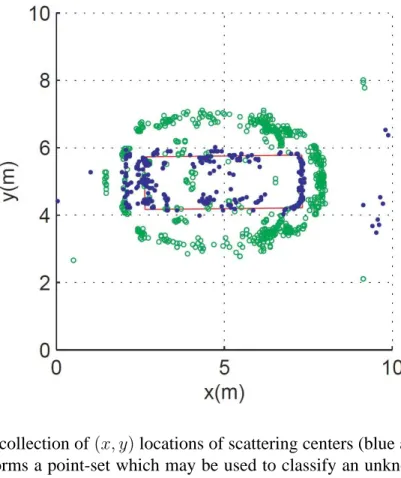
Figure 1.2: The collection of(x, y)locations of scattering centers (blue and green dots) in a radar image forms a point-set which may be used to classify an unknown target. Here, points were derived from a radar image of a Toyota Camry. Image source: [7], Figure 5.

referred to as scattering centers—are identified as a collection of points. In addition to the scattering center locations, additional point-wise attributes of the targets are collected by the radar system. These include return polarization and amplitude, and observation azimuth and elevation angles. Additionally, polarization and layover at-tributes from2Dimages enable the extraction of3Dpoint locations, yielding target shape and size information [8].

As an example, Figure1.2 illustrates a 2D point-set corresponding to the scattering center locations on a Toyota Camry. The blue points are derived from the base shape of the Camry, which is highlighted with the red box, whereas the green points are derived from the roof line which has been layed over in the same direction as the radar [7].

(14)

occur-ring points within an image, however we may derive point features as the locations where interesting non–point-like behavior occurs, for example, the locations of large gradients or the locations of SIFT features. The derived locations of these features may be collected into point-sets and used in classification. This approach has been used to identify categories (e.g., office, street, forest) of natural scenes [19].

1.2

Optimal Feature Selection

1.2.1

Motivation

Feature selection is the process of eliminating redundant and irrelevant data while maintain-ing the basic structural information of a model. In the context of point-set classification, we consider individual points in a training set as features. Identifying the most salient points required for classification and eliminating less salient points serves two purposes:

1. Reducing the size of the training database has the potential to dramatically accelerate test-time classification rates as seen in, for e.g., the partial match score (1.2).

2. Eliminating extraneous training data serves to regularize the classifier and provides robustness to limited and noisy data.

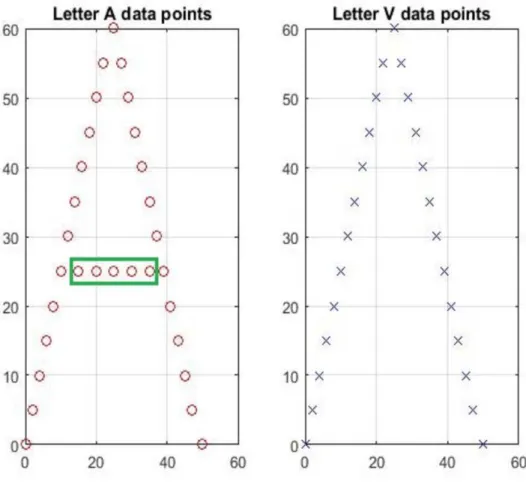
In Figure1.3, we present a simple example of redundant features in a point-set clas-sification problem. Here the goal is detect whether points belong to the letter A or (an upside down) V. Because all of the points of V are contained in A, these points are inca-pable of distinguishing between the two letters. Thus, only the points within the horizontal bar of A (highlighted by a green box) are expected to be salient to this classification task. In realistic problems, patterns are not simply repeated among classes making salient point identification more difficult. Increasing the number of classes also increases the complexity

(15)

Figure 1.3: Simple feature selection example for point-set classification. In classifying between the letters A and V, the points in V are completely redundant with those in A. Only the horizontal points in A (green box) are expected to be salient for this task.

of the problem because points that are not useful for some pairs of classes may be useful for others. In Chapter4we revisit this example while demonstrating the application of our op-timal feature selection algorithm. The following section provides a taxonomy of statistical feature selection methods.

1.2.2

Approaches

For a given feature setF ={f1, . . . , fN}, the goal of feature selection is to select a subset S ⊂F for use in classification, whereShas been chosen based on some optimality criteria. A least redundant subset ofF may be defined as the smallest subsetS0 ={s1, . . . , sn}such

(16)

that when any new featurer∈F is considered

P(S, r) =P(S). (1.3)

That is, the probability distribution ofS is equal to that of the probability distribution of (S, r), meaning thatris a complete derivative ofS. However, the least redundant subset is not necessarily the best subset for classification.

Information theoretic measures are often used to evaluate a feature’s significance [13]. Ifθ ∈ {1, . . . , L}is an unknown class label, we may consider the information gain provided by a setS of features

IG(θ|S) = H(θ)−H(θ|S). (1.4)

Here,H(θ)denotes the entropy ofθ

H(θ) =−X i

p(θi) log(p(θi)), (1.5)

andH(θ|S)is the entropy of the class labelθ after observingS, as given below

H(θ|S) =−X j p(Sj) X i X i p(θi|Sj) log(p(θi|Sj)). (1.6)

Using the information gainIG(θ|S), it is possible to evaluate and choose an optimal feature setSwhich minimizes the classification uncertainty overθ. WhenθandSare independent, H(θ|S) = H(θ), and the information gain from feature setSis zero.

Generally, feature selection methods may be categorized into three types [13]: wrap-per methods, filter methods, and embedded methods. Wrapwrap-per methods consider a global cost criterion that is used to evaluate any subset of features; for example the information gain (1.4), if we allowSto be any subset of features. Wrapper methods attempt to evaluate

(17)

the global cost over all possible subsets to identify the optimal selection. This process may include brute-force enumeration or more intelligent search strategies. Filter methods eval-uate and rank each feature independently, which can be significantly faster than searching over all subsets. For linear feature dependency and ranking, correlation between a feature fi and the class θ may be used. Information gain may be used in the filtering method if the setSin (1.4) is restricted to a single featurefi at a time. After ranking all features, the top n may be selected for use in classification. Finally, embedded methods combine the processes of variable selection and model fitting into a single process that is performed at the time of training.

As described in Chapter3, our approach to optimal point-feature selection is consid-ered an embedded method.

1.3

Contributions and Organization of the Thesis

The remainder of this thesis is organized as follows. In Chapter 2, background literature of the thesis is given. Here, an overview of spatial pyramid histograms is provided, and we present a computationally efficient approximation of the partial match score called the pyramid match kernel.

Our first major contribution is presented in Chapter 3, where we combine pyramid histograms and logistic regression to produce a new point-set classifier with probabilistic outputs—suitable for use in fusion applications. In this chapter we also present our

sec-ond major contribution, which is an embedded optimal feature selection strategy based

on a sparsifying prior for logistic regression weights. This strategy provides significant compaction of point-set databases with minimal performance impact.

(18)

applica-tion and analysis of our new point-set methods to the problem of fingerprint identificaapplica-tion. Here, we use measured data provided jointly by NIST and the FBI. Finally, conclusions and future work are provided in Chapter 5.

(19)

Background

While optimal, the partial match score (1.2) is generally not used in practice due to its computational complexity. In this chapter we review a popular approximation to the partial match score called the pyramid match kernel, which is based on a point-set representation called the spatial pyramid histogram.

2.1

Overview of Spatial Pyramid Histograms

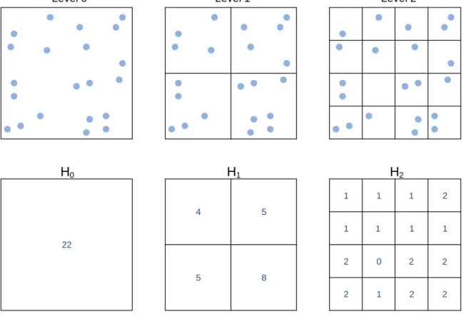
The concept of the spatial pyramid histogram (PH) was first introduced by Grauman and Darrell [11]. It is a multidimensional and multiresolution data structure that captures the distribution of a set of spatial points. As illustrated by the example in Figure2.1, the PH is a collection of multidimensional histograms of varying bin sizes and numbers. The largest level has the most bins and therefore has the highest resolution (Fig.2.1: Level 2 has4×4 bins). At each subsequently smaller level, the number of bins in each dimension is halved. In the example, this yields a2×2bin array for Level1, and a1×1bin array for Level0. The number of bins per dimension for levelℓis2ℓ_{, and if there are}_d_{dimensions, the total} number of bins in levelℓis

(20)

The example in Figure2.1has points in two dimensions,d= 2.

When the number of bins are halved in going to smaller levels, the size of the bins are doubled such that the total area covered does not change. In this way, for each dimension, two bins are combined into one larger bin covering the same area. This effects a halving of the resolution for each subsequently smaller level without changing the coverage area.

For a point-set Pt = {p1, . . . ,pNt}, pi ∈ R

d_{, the histogram counts for level} _ℓ _are denotedHℓ(Pt), as illustrated in the bottom row of Figure2.1. For anL-level PH, these varying resolution histograms are collected as

H(Pt) = [H0(Pt), H1(Pt), ..., HL(Pt)]. (2.2)

As illustrated in Figure2.2, when the per-level histogram counts are organized verti-cally, with the highest resolution (largest level number) counts on the bottom, the collection resembles a pyramid—thus yielding the name spatial pyramid histogram.

2.2

Pyramid Match Kernel

The Pyramid Match Kernel (PMK) [11] is a computationally efficient alternative to the partial match score (1.2). Like the PMS, the PMK quantifies the similarity of two point-sets in a way that solves the unknown correspondence problem and is robust to missing or displaced points within either set. Rather than being a function of point-sets directly, the PMK

(21)

Level 0 Level 1 Level 2 2 1 2 2 2 0 2 2 1 1 1 1 1 1 1 2 5 8 4 5 22 H0 H1 H2

Figure 2.1: Example of spatial histograms. Top row: At each successive level, the number of bins is doubled while the bin size is halved in each dimension. Dots indicate locations of points in the point-set. Bottom row: Histogram counts for each level.

Figure 2.2: Organizing the multi-resolution histograms vertically yields a spatial pyramid histogram.

(22)

is a function of the pyramid histograms derived from given point-sets P1 and P2. As a

measure of similarity, the PMK is larger for point-sets that are more alike. The PMK is computed as K(H(P₁), H(P₂)) = L X ℓ=0 wℓIℓ, (2.4) where Iℓ = 2dℓ X i min(H_ℓ(i)(P1), Hℓ(i)(P2)) (2.5)

indicates the number of intersections betweenP₁andP₂ among all2dℓ_{bins at level}_ℓ_{of the} histograms, andH_ℓ(i)(Pk) denotes the number of points counted in biniof pyramidPk at levelℓ. For each celli, the intersection considers the number of points in common between the two histograms, which is determined by the minimum count between the two point-sets. From (2.4), the PMK is computed as a weighted sum of the number of intersections observed at all of the levels.

The weights {wℓ} are parameters of the PMK and are generally chosen to reward matches at finer resolutions more than coarse ones. This is because two points falling into a finely resolved bin location is less likely to occur by chance and thus indicates a greater similarity between two point sets. As the histograms go from fine to coarse, more matches (intersections) will naturally occur, so such matches are weighted lower in indicating simi-larity. At the coarsest level (ℓ = 0), all the points in each point-set will be contained in the single bin at the top of the pyramid histogram. Here,Iℓ reaches its maximum and is equal to the minimum number of points betweenP₁ andP₂. Correspondingly, w₀ should be the lowest weight among all levels.

(23)

cost [12]. Hence, the maximum distance between two points sharing the same bin can not exceed the sum of lengths of the bin’s sides. In going from fine to coarse scales, a common weighting scheme [19] halves the weight each time the bin sizes double. We adopt the following per-level weight assignment

wℓ = 1

2L−ℓ, ℓ= 0,1, . . . , L (2.6)

which follows this halving strategy.

The distribution of point-features will vary in different applications. Therefore, the possible bin sizes and number of levels L should be considered specifically for each ap-plication. This concept is further illustrated in the context of fingerprint identification in Chapter4.

2.2.1

Pyramid Match Kernel Example

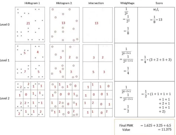
In this section, we present a detailed example of evaluating the Pyramid Match Kernel (PMK) between two point-sets. The specifics are presented in Figure2.3. The first column represents the first pyramid histogram, and the second column represents the second pyra-mid histogram. In the example, we consider a maximum of L = 2 levels. By inspecting Level 0, we see that the first point-set contains 21 points, while the second contains only 13 points. The count of the total number of points in a cell gives the bin value for that cell. The third column in the figure shows the result of computing the intersection (2.5) be-tween corresponding cells in the two histograms. We see that the intersection is computed as the number of points in common between cells, i.e. it is minimum between associated cells.

(24)

Figure 2.3: A detailed example of Pyramid Match Kernel evaluation between two pyramid histograms withL= 2maximum levels.

The level-dependent weights (2.6) and scores are given in the last two columns of Figure2.3. Finally, the summation of the level-weighted scores yields the final PMK value. As shown at the bottom of the figure, for this example the final PMK value was11.375.

(25)

2.3

Pre-processing Point Patterns

2.3.1

Local Neighborhood Selection

Before the existence of powerful computational tools, Fix and Hodges (1951) introduced the nearest neighbors concept with various other contemporary relevant topics [2]. The K-nearest neighbors (KNN) algorithm [14] is one of the simplest machine learning algorithms implemented for both regression and classification. In classification, it is based on a nearest neighbor decision rule in which a classification input sample point is decided based on previously classified training points. Hence, it is a memory based algorithm.

Here, following [8], we use a KNN-like strategy to define local neighborhoods around training points. For each pointp0 in a training pattern, we identify theK closest points in

the point-set based on the Euclidean distance betweenp0 and its neighbors

di =kpi−p0k. (2.7)

In this way, a size-K neighborhood of points is established for all points within a given class. Each of these neighborhoods will subsequently be represented by a pyramid histogram after an orientation equalization to be described next.

2.3.2

Translation and Orientation

In point-set classification, it is desirable to have robustness to the orientation of observed points. It is important to understand how data are obtained during the training and testing phases and how these differences are accounted for during classification. In this work, we assume that each point has an orientation attribute in addition to its spatial location, e.g.,

(26)

for two spatial dimensions a minimal representation of pointpi would be

(xi, yi, θi), (2.8)

where θi represents the orientation. Many applications have orientation attributes. For example, in the fingerprint application described in Section1.1.1, the minutia points have natural orientations describing the angles of ridge-ending and bifurcation split angles. In the radar application of Section 1.1.1, the orientation angle represents the angle at which the radar observes bright backscattered energy.

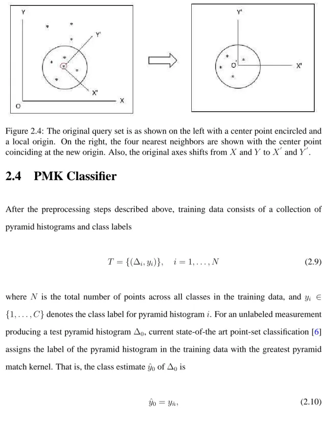
To develop robustness to differences in observation angles between training and test-ing, we follow [6] and transform each neighborhood of K + 1 points into a new local coordinate system. For a training pointpi, with features(xi, yi, θi), we translatepi and its K neighbors such thatpi resides at the new origin and all(K+ 1)points are rotated about the new origin by−θi. Figure2.4presents an example forK = 4.

Since training and testing points are similarly clustered and framed in their own local coordinate systems with orientation corrections, the point matching process becomes in-variant to the actual observation angles during measurement, and by looking for matches between small clusters of points, we achieve greater robustness to missing points.

In total, preprocessing consists of3steps, for each pointpi:

1. LocalK-neighborhood selection

2. Translation and rotation to center and orientpi

3. Pyramid histogram formation on the transformed cluster,Hi =H(pi)

We denote the resulting pyramid histogram for pointpi as∆i = H(pi), without explicitly indicating the neighborhood selection and transformation steps.

(27)

Figure 2.4: The original query set is as shown on the left with a center point encircled and a local origin. On the right, the four nearest neighbors are shown with the center point coinciding at the new origin. Also, the original axes shifts fromX andY toX′ andY′.

2.4

PMK Classifier

After the preprocessing steps described above, training data consists of a collection of pyramid histograms and class labels

T ={(∆i, yi)}, i= 1, . . . , N (2.9)

where N is the total number of points across all classes in the training data, and yi ∈ {1, . . . , C}denotes the class label for pyramid histogrami. For an unlabeled measurement producing a test pyramid histogram∆0, current state-of-the art point-set classification [6]

assigns the label of the pyramid histogram in the training data with the greatest pyramid match kernel. That is, the class estimateyˆ₀of∆0 is

ˆ

(28)

where

ˆ

n= arg max

n:1,...,NK(∆0,∆n). (2.11)

In practice, each point from an unknown target will produce an pyramid histogram and a class estimate. The collection of these estimates may be combined into a single point-set estimate via a majority-vote procedure. In this thesis, we focus on feature selection and optimal classification of a single pyramid histogram and not the fusion problem. The baseline against which we will compare our performance is the PMK classifier (2.10).

(29)

Optimal Feature Selection

Although state-of-the-art, the PMK classifier has drawbacks in that both database size and classification complexity grow linearly with the number of pointsN in the training dataset. This complexity motivates us to identify and use only the most salient features—thereby minimizing both of these costs. Further, by identifying and pruning less informative points, we achieve robustness to potential outliers in the training set.

Our approach is based on logistic regression, which has the side benefit of producing posterior class estimates. In the subsequent sections, we describe how logistic regression and the PMK may be combined into a point-set classifier and how a sparsifying prior may be used to identify salient features.

3.1

Multinomial Logistic Regression

A logistic regression model [16] employs the logistic function to predict the relationship between a categorical dependent variable y and one or more independent variables, or features. For a binary classification problem y ∈ {1,2}, with a d-dimensional feature vectorx,

(30)

-4 -3 -2 -1 0 1 Feature 1 -3 -2 -1 0 1 2 Feature 2

Figure 3.1: Logistic regression example for a two class problem: blue vs. red circles. The decision boundary is linear in the feature space.

where

σ(z) = 1

1 + exp(−z) (3.2)

is known as the logistic function, whileβ0andβ ∈Rdare parameters learned from training

data. The complement probability may be shown [16] to be

P(y = 2|x) = 1−σ(β₀ +βTx) (3.3)

=σ(−β0−βTx) (3.4)

= 1

1 + exp(β₀+βT_x₎. (3.5)

Logistic regression is a linear classifier as shown by the example in Figure3.1.

(31)

represented as below [14] p(y = 1|x) = exp(β10+β T 1x) P kexp(βk0+β T kx) p(y = 2|x) = exp(β20+β T 2x) P kexp(βk0+βkTx) .. . p(y =C|x) = exp(βC0+β T Cx) P kexp(βk0+βkTx) . (3.6)

The parameters θ = {β10, β1, . . . , βM0, βM} in the model may be learned using training data, and we writep(y|x, θ)to explicitly indicate the dependence of the classifier on these parameters. After an estimateθˆofθis obtained, we may classify a new feature vectorxtest using maximum a posteriori (MAP) classification as

ˆ

y = arg max

y:1,...,Cp(y|xtest, ˆ

θ). (3.7)

To learn the parameters, a set of training data

(xi, yi), i= 1, . . . , N (3.8)

is used. Here, the {xi} are d-dimensional feature vectors and yi ∈ {1, . . . , M} is the class label for sample i. Assuming the training data consists of independent samples, the likelihood of the data is formed as

L(θ) = N

Y

i=1

(32)

and, using (3.6), the log-likelihood as ℓ(θ) = N X i=1 logp(yi|xi, θ) (3.10) = N X i=1 (βyi0+β T yixi)− N X i=1 log C X m=1 eβm0+β T mxi ! . (3.11)

Maximum likelihood parameters are found from the training data as

ˆ

θ = arg max

θ ℓ(θ). (3.12)

The optimization (3.12) may be efficiently performed using coordinate descent and a quadratic approximation to the log-likelihood considering one class at a time [15].

3.2

Logistic Regression for Point-set Classification

Logistic regression can not be directly applied to point-set classification because the num-ber of points in measured imagery is variable and, like most classification methods, logis-tic regression requires a fixed-length feature vector. In this section we describe how the pyramid match kernel may be combined with multinomial logistic regression to solve this problem.

Instead of developing and using a fixed-dimensional feature space, we utilize a memory-based classifier that compares a new collection of points to all points seen in the training set. This is similar to theK-nearest neighbor algorithm and the PMK classifier described above. Similar to the PMK classifier, we will use the pyramid match kernel as a measure of similarity between pyramid histograms. However, rather than adopting the label of the training element with the largest PMK value, we utilize a weighted combination of kernel

(33)

scores across the entire saved training set. This provides robustness to potential outliers in the training set and enables us to evaluate the contribution of particular points among the training data.

Specifically, we utilize a kernel-based classifier that replaces the features in traditional logistic regression with PMK scores computed between a pyramid histogram under test and the full training database. Following the pre-processing steps described in Section2.3, we have a collection of training pyramid histograms and their associated class labels

(∆i, yi), i= 1, . . . , N. (3.13)

For an unlabeled pyramid histogram under test,∆0, we compute weighted logistic

regres-sion scores with respect to every element in the training set using the PMK. Thekth score is computed as zk =βk0+ N X n=1 βkiK(∆0,∆i), k= 1, . . . , C (3.14)

whereK(∆i,∆j)denotes the PMK (2.4) between pyramidsiandj; andCis the total num-ber of classes. With kernel-derived scores replacing feature-based scores, the multinomial logistic regression posterior probabilities (3.6) take the form

p(y= 1|∆0) = exp(z₁) PC k=1exp(zk) p(y= 2|∆0) = exp(z₂) PC k=1exp(zk) .. . p(y=C|∆0) = exp(zC) PC k=1exp(zk) . (3.15)

(34)

In (3.14), βk0 represents the scalar intercept for classk, while{βki}Ni=1 represent the

weights for classk against allN elements in the training set. In total, there areC+CN parameters that need to be learned using the training data (3.13). After computation of the kernel distances between all pyramid histograms in the training data, theβparameters may be learned using maximum likelihood identically to the non-kernel-based form in (3.12).

3.3

Feature Selection

One advantage of the logistic regression classifier is that the weights (β’s) may be used to identify important points in the training data. From (3.14), we see that if|βki|is large, then ∆i(corresponding to pointiin the training data) plays a relatively large role in determining the classification score zk. Thus, points with large coefficients may be considered more salient than points with small coefficients.

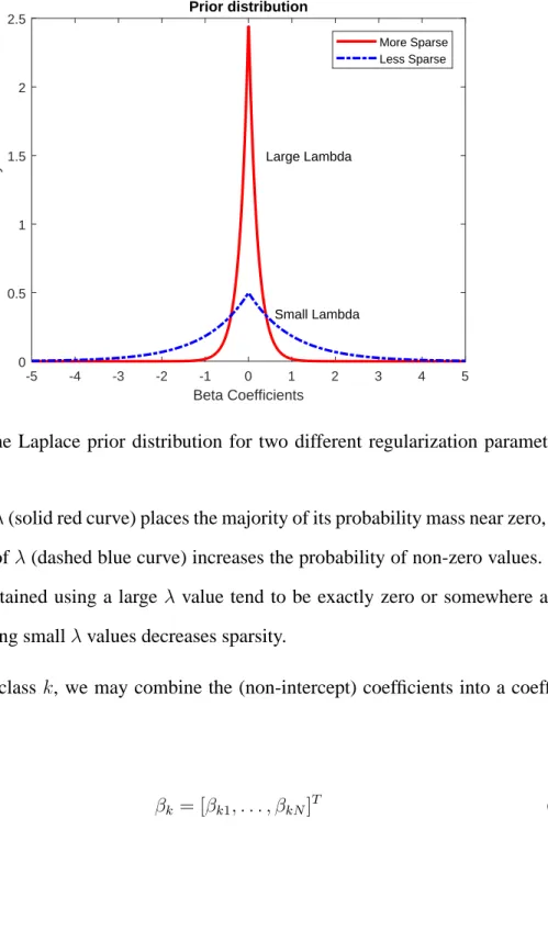
Taking this concept further, we can change our learning algorithm to generally assume that a point is not salient unless the data strongly supports otherwise. This belief can be incorporated through the use of a prior distribution on the coefficients and switching from maximum likelihood estimation (as in Eq. (3.12)) to maximum a posteriori (MAP) estimation. In order to encourage feature (point) reduction, we choose a prior that favors coefficient values of zero—indicating that the feature is non-salient. Such a prior is often termed a sparsifying prior because the resulting estimated coefficients are generally sparse: having only a few non-zero elements. A common sparsifying prior [3] is the Laplace distribution

p(β) = λ 2e

−λ|β|_. _(3.16)

(35)

-5 -4 -3 -2 -1 0 1 2 3 4 5 Beta Coefficients 0 0.5 1 1.5 2 2.5 Density Prior distribution Large Lambda Small Lambda More Sparse Less Sparse

Figure 3.2: The Laplace prior distribution for two different regularization parameter (λ) values.

large value ofλ(solid red curve) places the majority of its probability mass near zero, while a small value ofλ(dashed blue curve) increases the probability of non-zero values. Thus, coefficients obtained using a large λ value tend to be exactly zero or somewhere around zero, while using smallλvalues decreases sparsity.

For each classk, we may combine the (non-intercept) coefficients into a coefficient vector

(36)

and impose the Laplace prior on each element independently p(βk) = N Y i=1 p(βki) (3.18) = λ 2 N e−λPi|βki| (3.19) = λ 2 N e−λ||βk||1 , (3.20)

where|| · ||1 denotes the vectorℓ1norm.

Lettingγi = [K(∆i,∆1), . . . , K(∆i,∆N)]T denote the vector of PMK values evalu-ated between featureiand all features in the training setT, the kernelized logistic regres-sion likelihood is L(T|θ) = N Y i=1 p(yi|γi, θ) (3.21) = N Y i=1 exp(βyi0+β T yiγi) PC m=1exp(βm0+βmTγi) . (3.22)

Combining this with the prior onθ = [β₁₀, β₁, . . . , βC0, βC]T,

p(θ) = C

Y

m=1

p(βm), (3.23)

the posterior over the parameters is

p(θ|T)∝L(T|θ)p(θ). (3.24)

(37)

depend onθ. After substituting (3.22) and (3.24), we obtain ℓ(θ) = N X i=1 (βyi0+β T yiγi)− N X i=1 log C X m=1 eβm0+β T mγi ! −λ C X m=1 ||βm||1 (3.25)

as the final objective to be minimized. This yields

ˆ

θ = arg max

θ ℓ(θ) (3.26)

as the MAP estimate for the optimal logistic regression parameters.

The last term in (3.25) is theℓ1 penalty that penalizes non-zero coefficients and

pro-motes sparsity. This is also referred to as the Least Absolute Shrinkage and Selector Op-erator (LASSO) penalty as used in LASSO-type regression problems[14]. In [25], the equivalency between LASSO regression and Laplacian priors is explored in more detail.

There are a number of sparsity-based algorithms discussed in, e.g., [26] [17] [1] [15] [4] [23] capable of optimizing penalized objectives similar to (3.25). A cyclic coordinate descent algorithm based on a regularizaton path is described in [15]. We used a particu-lar implementation of this method, referred to as GLMNET [24], to optimize (3.25) and produce the results presented in Chapter4.

As noted earlier, when particular coefficients are zero, associated points do not enter into the logistic regression scores used in classification. Therefore, after optimizing the weights (3.26) using GLMNET, if weightβki = 0, then feature (pyramid histogram)ican be excluded when computing the logistic regression score for classk. However, because the posterior over all classesk ∈ {1, . . . , C}must be computed before a most likely class can be identified, eliminating a point is only useful if it is eliminated from all class posterior calculations. Otherwise, the point cannot be removed from the training database. This may

(38)

be expressed by constraining groups of parameters to simultaneously be zero:

βki = 0 =⇒ βkj = 0, ∀j ∈ {1, . . . , N}. (3.27)

This constraint is referred to as group sparsity and is enforced in GLMNET using the option ‘grouped’.

Following a group sparse solution to minimizing (3.25), all featuresiwhereβki = 0, for any k, may be eliminated from the database used at test time. In Chapter 4 we ex-plore how many points may be removed from the database without impacting classification performance.

3.4

Sparsity Selection

In the objective function (3.25), the variableλ ≥ 0is referred to as the regularization pa-rameter. This parameter controls the severity of the penalty applied to non-sparse solutions, and as illustrated in Figure3.2, large values ofλproduce sparser solutions than small values ofλ. Forλ = 0there is no penalty, and we obtain a non-sparse estimate equivalent to the maximum likelihood solution. Accordingly, the value ofλ controls the tradeoff between database reduction (sparse solutions) and classification performance. Properly selectingλ is an important component in the overall process of selecting the most salient points.

Cross-validation [27] is a method to choose the regularization parameterλsuch that it minimizes an estimate of the prediction error. An ideal scenario would have ample amounts of training and testing data. However, when data is limited, cross validation may be applied to divide the original data into multiple training and testing sets. We employK-fold cross-validation which splits data intoK groups. First, K −1 groups are used to train the pa-rameters, while remaining held-out group is used as a testing set to evaluate the prediction

(39)

217 200 175 150 120 105 81 59 40 28 14 0 Degrees of Freedom -10 -9 -8 -7 -6 -5 -4 -3 -2 log(Lambda) 0 5 10 15 20 25 Multinomial Deviance

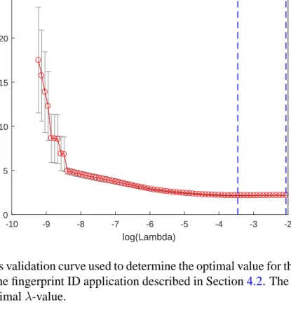
Figure 3.3: Cross validation curve used to determine the optimal value for the regularization parameterλin the fingerprint ID application described in Section4.2. The left vertical line indicates the optimalλ-value.

error. The procedure is repeatedK times, holding out a different set each time. The results are combined to form an estimate of the prediction error as a function of λ. Finally, the optimal regularization parameter is chosen as the one that minimizes the cross-validation prediction error estimate. In our work, we used10-fold cross validation to determineλ. A sample cross-validation curve is illustrated in Figure3.3for the fingerprint ID application considered in the next chapter.

(40)

Results and Analysis

4.1

Character Recognition Example

Previously, in Chapter 1, we considered a simple character recognition example between the letters “A” and “V” to provide intuition about the optimal selection of point features. In this section, we present the results of applying our optimal feature selection process to this problem.

During the training process, our model should generalize such that salient behavior associated with the data is captured. When the learned model is too simple, we experience underfitting characterized by high bias and low variance. Overly complex models fit the data too well and learn noise within the data as well [21]. These two undesired training phenomenon yield poor performance.

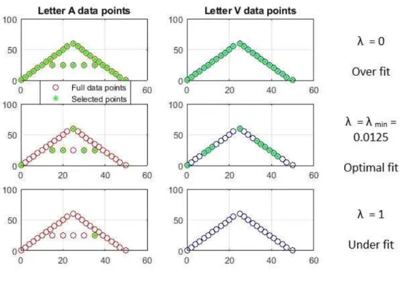
As described in Section3.4, we utilize the sparsity parameterλto control regulariza-tion and set this value using cross validaregulariza-tion. Initially, we trained the both “A” and “V” classes without any regularization (λ = 0). As expected, the algorithm selects all of the data without giving any further idea on usefulness of data points among the two characters. This is illustrated by the top row of plots in Figure4.1.

The bottom row of plots in Figure4.1 depicts a large value ofλ which removes too many points from the training data and underfits the data. The middle row of plots in

(41)

Figure 4.1: Optimal point selection example. When the regularization parameterλ is too small (upper row) too many points are selected; and whenλis too large, salient points are omitted (bottom row). The optimal value (middle row), determined by cross-validation, balances this trade-off and selects only the most discriminative points. Selected points are denoted by green asterisks.

Figure4.1represents the optimal level of regularization as determined by cross validation. As hypothesized in the Introduction, the bar of the letter “A” is selected, however certain other points are also selected. In the letter “V” these points are adjacent to where the A-bar would have been. From this, we conclude that the algorithm is looking for edge diagonals and an absence of the “bar” to identify the letter “V”.

For this example, we conducted a noiseless simulation to empirically evaluate the probability of correct classification (PCC). Using all of the features (λ = 0), we obtained PCC=76.67%, and while using only sparsely identified features (optimalλ) we obtained PCC=73.33%. This demonstrates our algorithm’s capability of identifying the most salient features. In the following section, we apply our algorithm to noisy measured data from a fingerprint ID application.

(42)

4.2

Fingerprint Recognition Data

4.2.1

NIST SD 27 Database

The NIST SD 27 database [9] was developed by the National Institute of Standards and Technology (NIST) in coordination with the Federal Bureau of Investigation (FBI). It con-tains gray scale fingerprint images and their corresponding characteristic point features data called minutia. An example image is shown in Figure4.2. There are 258 latent fingerprints from the crime scenes together with their matching tenprint images. For each finger, there are different sets of minutiae. One of the sets contains all the minutiae coordinates on the latent; another contains all the minutiae points from its tenprint while there is another set with all common minutiae between these latent and tenprint sets.

Since the latent minutiae were collected from a real-world scene, they have the poorest quality and generally only contain a subset of minutiae of a corresponding tenprint. Based on the quality of the image, all the fingerprint sets have been further categorized into good, bad and ugly directories with good being the best quality.

All the fingerprints are composed of two basic focal points in the form of loops and/or whorls that help to distinguish each minutia set. These focal points are called core with a loop and delta for the one with a whorl. These minutia attributes in the fingerprint are also termed as ridge ending and ridge bifurcation. To find a match, we desire to match these points from a latent minutia with a database formed from tenprints.

Each minutia is represented in terms of its location and orientation in the image. All the images in our database are of size800×768 pixels, where each pixel represents0.01 millimeters in both the ANSI/NIST standard and the FBI EFTS [9]. For positioning the origin, the bottom left of the image is considered its origin in the ANSI/NIST standard, while FBI/IAFBIS has its origin at the top left of the image. Due to this discrepancy,

(43)

100 200 300 400 500 600 700 800 100 200 300 400 500 600 700 320 340 360 380 350 400 450 500

Figure 4.2: A typical “tenprint” image from the NIST SD 27 fingerprint database. Major detected minutia (red circles) and associated orientations (magenta lines) of the fingerprint are shown.

the X-coordinates are the same for both standards, while there is a linear inversion of the Y-coordinates.

4.2.2

Bin Size Determination

In order to compute the pyramid histograms described in Section2.1for the minutia points in the fingerprint database, we need to establish the bin sizes at the lowest level of the pyramid histogram. The bin sizes at the upper levels are a function of the lowest level. The smallest bin size controls a tradeoff between faithfully capturing low-level patterns and providing high-level clustering that is robust to missing and occluded points.

To determine the bin sizes, we computed 1D histograms of the X and Y distances from every training point and its five nearest neighbors. These histograms are shown in Figure4.3. Since the vast majority of points fall within ±5mm of one another, we chose

(44)

Figure 4.3: Histograms of nearest-neighbor distances determine the bin sizes used while generating pyramid histograms.

the smallest bin size such that the 2D spatial histogram area covers this 10mm×10mm area.

4.3

Fingerprint Experiments and Results

In this section, we report the results from several classification experiments that were car-ried with the NIST SD 27 database. For the training data, we used tenprint data taken in a controlled environment; and for testing data we used field-measured fingerprints labeled as “good.” We used the good data to establish a performance baseline. From this point, we can artificially introduce additional noise and obscurations in a controlled manor to further evaluate performance. In all cases below, we use the probability of correct classification (PCC) as the performance metric. As a benchmark, we will often compare to the PMK classifier (Section 2.4) which utilizes the full set of training data. We refer to this as the

(45)

2 2.5 3 3.5 4 4.5 5

Pyramid Histogram Level, L

0 200 400 600 800 1000 1200 1400 1600 1800

Time taken in seconds

Cost of higher pyramid level

Figure 4.4: Time required to compute pyramid histograms for the entire training database versus maximum number of levels,L. Large values ofLrequire excessively long compu-tation times.

“full” data benchmark.

However, before evaluating feature selection performance, we use the fingerprint dataset to explore two implementation parameters of pyramid histograms: the number of levels (L) and the local neighborhood size (K).

4.3.1

Number of Pyramid Histogram Levels

Increasing the maximum number of Pyramid Histogram levels, L, increases the resolu-tion at the bottom level of the pyramid histogram and improves the granularity of partial matches. The tradeoff of increasingL, however, is the computational cost required to com-pute the 2D histograms at a larger number of levels. Further, this complexity is not linear inLbecause, from (2.1), the number of bins increases by a factor of2d_{for each additional} level. Here dis the dimensionality of the points. For the fingerprint application, we have

(46)

2 2.5 3 3.5 4 4.5 5

Pyramid Histogram Level, L

91.5 92 92.5 93 93.5

Percentagee Correct classfication

Figure 4.5: Performance of the PMK classifier as a function of the maximum number of pyramid histogram levels,L.

d= 2and expect a 4-fold increase in complexity for each additional level.

In Figure4.4, we report the time required to compute the pyramid histograms for all 307 points in the full training data. The figure considers a maximum number of levels ranging fromL = 2toL = 5, and the exponential time increase is readily apparent. Fur-ther, while we don’t report values here, storage requirements and test-time computational complexity would increase similarly withL.

Given the dramatic increase in complexity with L, we next evaluated the resulting benefit afforded by largerLvalues. Using the benchmark PMK classifier (Section2.4), in Figure4.5we report PCC vs. L. Somewhat surprisingly, for the fingerprint data under con-sideration, we do not observe any performance increase withL. We believe this is because the minutia are roughly uniformly distributed andL = 2provides sufficient resolution for each minutia point to reside in its own bin at the lowest level. As such, we useL = 2for the remainder of our experiments.

(47)

4 6 8 10 12 14 16 18 20

Number of nearest neighbors

65 70 75 80 85 90 95 100

Percentagee Correct classfication

Sparse PMK

Figure 4.6: Classification performance versus local neighborhood size,K.

4.3.2

Local Neighborhood Size

A second implementation choice is the sizeK of the local neighborhoods (see Sec.2.3.1) that are used to form pyramid histograms. Increasing K decreases the probability that a random collection of points will match a true point-set, however as K increases more points are likely to share histogram bins, thus decreasing the uniqueness of a quantized histogram representation. We also note that for small datasets it may be impossible to use very large values ofK as there simply may not be that many points in the global data.

In Figure4.6, usingL= 2maximum levels, we plot PCC versus theK for the PMK classifier and our sparse logistic regression classifier. For this fingerprint data, and both classifiers, neighborhood sizes less thanK = 7seem appropriate. For subsequent experi-ments, we useK = 5local neighbors.

(48)

Full Sparse 0 50 100 150 200 250 300 350 Number of Features

Figure 4.7: The proposed sparsity-based optimal feature selection algorithm reduces the full dataset by 94%, from 307 pyramid histograms to 19 pyramid histograms identified as being salient.

4.3.3

Optimal Feature Selection

In this section, we evaluate the size of the optimal feature set selected by our algorithm and present the corresponding classification performance. Our goal is to compare the perfor-mance of our sparse feature set to that obtained using the full dataset. As depicted by the bar graph in Figure4.7, the original “full” dataset contained 307 features. The number of salient features, identified by our algorithm as the non-zero coefficients obtained after cross validation, was only 19. This represents a 94% decrease in the database size.

The corresponding classification performance is reported in Figure4.8. Here we see that the baseline max kernel classifier (Section 2.4) that uses all of the data has a PCC of only 57%. Our non-sparse logistic regression method, which also uses all of the training data, has a PCC of 83%. This improvement is due, in part, to the fact that the logistic regression classifier makes its decision as a weighted combination of information in the

(49)

Figure 4.8: Classification performance of the proposed logistic regression methods (full and sparse) and the baseline max-Kernel classifier of Section2.4. While using 94% fewer features, the proposed sparse method outperforms the baseline which uses all of the training data.

entire training set and is less susceptable to outlier noise affecting single elements in the training data. Finally, our sparse classifier, which uses only 6% of the total training data, achieves a PCC of 69%. This is better than the baseline full data classifier, but not as good our own full data classifier.

4.3.4

Robustness to Limited Training Data

The training data used above was derived from high-quality tenprint images taken in a controlled environment. However, often such complete training is unavailable and we are obliged to classify with only partially data. To evaluate performance under these condi-tions, we randomly excluded points from the training set and plotted performance versus the percentage of features retained. Figure 4.9 illustrates the expected result that all al-gorithms experience degraded performance as training data is decreased. However, our

(50)

10 20 30 40 50 60 70 80 90 100 Percentage of features 0 10 20 30 40 50 60 70 80 90

Percentagee Correct classfication Full_Sparse

PMK

Figure 4.9: Percentage of correct classification versus training data retained. The proposed logistic regression methods (full and sparse) decay more gracefully in the presence of lim-ited training data.

proposed logistic regression based methods degrade much more gracefully. For example, while decreasing the number of training features by 30%, the proposed methods only suf-fer a PCC degradation of approximately 5%. For the same reduction in features, the PMK classifier has a performance reduction of approximately 15%.

4.3.5

Performance in Noise

Finally, we evaluate the performance of our algorithm in noise. For this experiment, we trained our classifiers using the original tenprint data. However, for the testing data, we added independent Gaussian noise to the minutia locations in order to shift them from their true locations. In Figure4.10we present these results as a function of the standard deviation of the additive noise. We observe that, in general, the noise has a significant impact on classification performance, however the proposed sparse method is slightly more robust to

(51)

0 0.5 1 1.5 2 2.5 3

Standard Deviation of Minutia Displacement (mm)

35 40 45 50 55 60 65 70 75 80

Percentage Correct classfication

Full Sparse

Figure 4.10: Percentage of correct classification versus standard deviation of minutia dis-placement. The proposed sparse method exhibits slightly more robustness to noise.

(52)

Conclusions

The crowning glory of the modern era depends on a broad range of innovations, from the basic tools to the most recent advancements in engineering where most of the smart gadgets stand. There is a desire to optimally process data to understand its characteristics more efficiently and accurately and to extract the most information possible. In this thesis, we designed an optimal feature selection algorithm for point-set classification based on efficient use of spatial pyramid histograms. Our algorithm identifies the most salient point features for use in a given classification problem which serves to reduce the complexity and increase the robustness of subsequent classification tasks.

We applied our algorithm to the NIST SD 27 database of fingerprints and demonstrated that only 6% of the original minutia point-features were salient. Using only the small salient dataset, we achieved classification performance superior to the current state-of-the-art method based pyramid match kernel maximization. The regularization and data-usage aspects of our classifier also yielded favorable robustness properties to noise and limited training data.

Finally, the logistic regression framework used in this thesis provides posterior probabilities for class memberships. In future work, this soft output may be used for fusion with other information sources. In particular, this work only considered classifying a single point and its local neighborhood. In practice, an object to be classified contains many point-like neighborhoods whose solutions may be fused to yield performance greater than the individual results reported in this thesis.

(53)

Bibliography

[1] Genkin Alexander, Lewis David D., and Madigan David. Large-scale bayesian logis-tic regression for text categorization. Technometrics, page 291, 2007.

[2] Silverman B. W. and Jones M. C. E. fix and j.l. hodges (1951): An important contri-bution to nonparametric discriminant analysis and density estimation: Commentary on fix and hodges (1951). International Statistical Review / Revue Internationale de

Statistique, 1989.

[3] E. J. Cand`es, J. Romberg, and T. Tao. Stable signal recovery from incomplete and inaccurate measurements. Comm. Pure Appl. Math., 59:1207–1223, 2005.

[4] Gavin C. Cawley, Nicola L. C. Talbot, and Mark Girolami. Sparse multinomial lo-gistic regression via bayesian l1 regularisation. Advances in Neural Information

Pro-cessing Systems 19, page 209, 2007.

[5] Richard O. Duda, Peter E. Hart, and David G. Stork. Pattern classification. Wiley-Interscience, New York, 2001.

[6] Kerry Dungan and Lee Potter. Classifying transformation-variant attributed point patterns. Pattern Recognition, 43:3805–3806, 2010.

(54)

[7] Kerry E. Dungan, Christian Austin, John Nehrbass, and Lee C. Potter. Civilian vehicle radar data domes. volume 7699, 2010.

[8] Kerry E. Dungan and Lee C. Potter. Classifying vehicles in wide-angle radar us-ing pyramid match hashus-ing. IEEE Journal of Selected Topics in Signal Processing, 5(3):577, 2011.

[9] Michael D Garris and R. Michael McCabe. Fingerprint minutiae from latent and

matching tenprint images. [microform]. NISTIR: 6534. Gaithersburg, MD : U.S.

Dept. of Commerce, Technology Administration, National Institute of Standards and Technology, [2000], 2000.

[10] K. Grauman and T. Darrell. Pyramid match hashing: Sub-linear time indexing over partial correspondences. In2007 IEEE Conference on Computer Vision and Pattern

Recognition, pages 1–8, June 2007.

[11] Kristen Grauman and Trevor Darrell. The pyramid match kernel: discriminative clas-sification with sets of image features. Tenth IEEE International Conference on Com-puter Vision (ICCV’05) Volume 1, ComCom-puter Vision, 2005. ICCV 2005. Tenth IEEE

International Conference on, Computer Vision, page 1458, 2005.

[12] Kristen Grauman and Trevor Darrell. The pyramid match kernel: Efficient learning with sets of features. Journal of Machine Learning Research, 8(4):725 – 760, 2007. [13] Isabelle Guyon and Andr Elisseeff. An introduction to variable and feature selection.

Journal of Machine Learning Research, 3(7/8):1157 – 1182, 2003.

[14] Trevor Hastie, Robert Tibshirani, and J. H. Friedman. The elements of statistical

learning : data mining, inference, and prediction. Springer series in statistics. New

York : Springer, c2009, 2009.

[15] Friedman Jerome, Hastie Trevor, and Tibshirani Rob. Regularization paths for gen-eralized linear models via coordinate descent. Journal of Statistical Software, Vol 33,

(55)

Iss 01 (2010), 2010.

[16] David G Kleinbaum and Mitchel Klein. Logistic regression. [electronic resource] :

a self-learning text. Statistics for biology and health. New York : Springer, c2010,

2010.

[17] B. Krishnapuram, L. Carin, M.A.T. Figueiredo, and A.J. Hartemink. Sparse multino-mial logistic regression: fast algorithms and generalization bounds. IEEE

Transac-tions on Pattern Analysis and Machine Intelligence, page 957, 2005.

[18] Alex Krizhevsky, Ilya Sutskever, and Geoffrey Hinton. Imagenet classification with deep convolutional neural networks. Communications of the ACM, 60(6):84–90, May 2017.

[19] S. Lazebnik, C. Schmid, and J. Ponce. Beyond bags of features: Spatial pyramid matching for recognizing natural scene categories. InProc. IEEE Computer Vision

and Pattern Recognition (CVPR), pages 2169–2178, Washington, DC, 2006.

[20] J. Marcum. A statistical theory of target detection by pulsed radar. Technical Report RM-754-PR, RAND Corporation, Santa Monica, CA, 1947.

[21] Stephen Marshland. Machine Learning : an algorithmic perspective. Chapman & Hall/CRC machine learning & pattern recognition series. Boca Raton, FL : CRC Press, [2015], 2015.

[22] Mark Mattson. Superior pattern processing is the essence of the evolved human brain.

Frontiers in Neuroscience, (8), 2014.

[23] Lukas Meier, Sara Van de Geer, and Peter Bhlmann. The group lasso for logistic re-gression. Journal of the Royal Statistical Society: Series B (Statistical Methodology), 70(1):53, 2008.

(56)

[24] J. Qian, T. Hastie, J. Friedman, R. Tibshirani, and N.

Si-mon. GLMNET for Matlab (2013). Stanford University, 2013.

http://www.stanford.edu/˜hastie/glmnet_matlab/.

[25] R. Tibshirani. Regression shrinkage and selection via the LASSO. Journal of the

Royal Statistical Society. Series B (Methodological), pages 267–288, 1996.

[26] Michael E. Tipping. Sparse bayesian learning and the relevance vector machine.

Jour-nal of Machine Learning Research, 1(3):211 – 244, 2001.

[27] Yongli Zhang and Yuhong Yang. Cross-validation for selecting a model selection procedure. Journal of Econometrics, 187:95 – 112, 2015.

CORE Scholar CORE Scholar

Browse all Theses and Dissertations

Theses and Dissertations