Mining Advertiser-specific User Behavior Using Adfactors
Nikolay Archak
New York University, Leonard N. Stern School of Business
44 West 4th Street, Suite 8-185
New York, NY, 10012
[email protected]
Vahab S. Mirrokni
Google Research 76 9th Ave New York, NY 10011[email protected]
S. Muthukrishnan
Google Research 76 9th Ave New York, NY 10011[email protected]
ABSTRACT
Consider an online ad campaign run by an advertiser. The ad serving companies that handle such campaigns record users’ behavior that leads to impressions of campaign ads, as well as users’ responses to such impressions. This is sum-marized and reported to the advertisers to help them eval-uate the performance of their campaigns and make better budget allocation decisions.
The most popular reporting statistics are the click-through rate and the conversion rate. While these are indicative of the effectiveness of an ad campaign, the advertisers often seek to understand more sophisticated long-term effects of their ads on the brand awareness and the user behavior that leads to the conversion, thus creating a need for the report-ing measures that can capture both the duration and the frequency of thepathwaysto user conversions.
In this paper, we propose an alternative data mining frame-work for analyzing user-level advertising data. In the ag-gregation step, we compress individual user histories into a graph structure, called theadgraph, representing local cor-relations between ad events. For the reporting step, we in-troduce several scoring rules, called theadfactors(AF), that can capture global role of ads and ad paths in the adgraph, in particular, the structural correlation between an ad im-pression and the user conversion. We present scalable local algorithms for computing the adfactors; all algorithms were implemented using the MapReduce programming model and the Pregel framework.
Using an anonymous user-level dataset of sponsored search campaigns for eight different advertisers, we evaluate our framework with different adgraphs and adfactors in terms of their statistical fit to the data, and show its value for mining the long-term behavioral patterns in the advertising data.
Categories and Subject Descriptors
H.4.m [Information Systems]: Miscellaneous; J.4 [Social and Behavioral Sciences]: Economics
General Terms
Performance, Measurement, Economics
Copyright is held by the International World Wide Web Conference Com-mittee (IW3C2). Distribution of these papers is limited to classroom use, and personal use by others.
WWW 2010, April 26–30, 2010, Raleigh, North Carolina, USA. ACM 978-1-60558-799-8/10/04.
Keywords
sponsored search, ad auctions, online advertising, PageR-ank, user behavior models, clickthrough rate, conversion rate
1.
INTRODUCTION
The Internet has become a major advertising medium. Although a number of different factors contributed to this, what distinguishes the Internet advertising from the offline advertising competitors is its inherently interactive nature. Measuring effectiveness of a particular advertising campaign and allocating the advertising budget optimally was and still remains a very challenging task, yet the Internet made the task easier by connecting ad impressions1 to tangible user actions and artifacts such as posing a search query, click-ing on an ad or convertclick-ing2. The simplicity of measuring and attributing user clicks has established the clickthrough rate (CTR) 3 as the current de-facto standard of ad qual-ity for sponsored search. It is now customary to define the advertiser’s optimization problem as maximization of the expected number of ad clicks given a certain budget con-straint [13, 23, 10]. The conversion rate (CR), defined sim-ilarly as the probability of the user conversion, is another popular ad effectiveness measure; together with the CTR it is frequently used by the advertisers to measure the re-turn on investment of specific keywords in the advertising campaign.
Recent empirical studies show that the effects of online ads cannot be fully captured by the CTR or the CR. In particu-lar, the sponsored search advertising, as well as the display advertising, can have a significant number of indirect effects such as building the brand awareness [18]. For instance, Lewis and Reiley [20], in cooperation between Yahoo! and a major retailer, performed a randomized controlled experi-ment to measure the effect of the online advertising on sales. They found that the online advertising campaign had sub-stantial impact not only on the users who clicked on the ads but also on those who merely viewed them. In another study, comScore [8] reported an incremental “lift” of 27% in 1Impression is simply an act of showing an ad in a page viewed by the user.
2Conversions are defined by the advertisers and may rep-resent a wide range of user activities from buying an item to simply spending a suitable amount of time on the adver-tiser’s website.
3The clickthrough rate (CTR) is defined as the fraction of times an ad was clicked by users when shown.
the online sales after the initial exposure to an online ad, as well as lift in other important online behaviors, such as the brand site visitation and the trademark searches.
The advertisers seek to understand the impact of their ad not just on the immediate click or conversion, but the likelihood of the eventual conversion in the long term and other long term effects. Users take specific trajectories in terms of the search queries they pose and the websites they browse, and this affects the sequence of ads they see; con-versely, the sequence of ads they see affects their search and browsing behavior. This interdependence results in struc-tural patterns in users’ behavior; advertisers need new tools and concepts beyond simple aggregates (like the CTR and the CR) to understand them.
What are the systematic ways to help the advertisers rea-son about structural correlations in the data? In this paper, we take an advertiser-centric data mining approach. We start with data that is directly pertinent to the advertiser’s campaign, that is, user trajectories that involved ads from the campaign of that advertiser, including ad impressions, clicks and conversions. Such data can usually be reported to the advertiser, provided it is aggregated and anonymized appropriately. Next, we build a data mining framework that can help advertisers identify structural patterns in this data. Our contributions are as follows.
• We propose a graphical model based approach. We formulate graphs from the data calledadgraphsto cap-ture co-occurrences of events adjacent to each other in users’ trajectories. Then, we introduce a variety of ad-factors, where every adfactor is a scoring rule for nodes in the adgraph: these are designed to capture impact of ad nodes on eventual conversion. For example, we introduce adfactors based on random walks, that, for every event, calculate the long term probability that a certain random walk involving that event would even-tually lead to conversion. Our paper presents highly ef-ficient algorithms for constructing adgraphs and com-puting all adfactors we introduce. All algorithms were implemented using MapReduce [11] parallel program-ming model.
• Using data from the sponsored search campaigns of eight different advertisers, we study various adgraphs and adfactors. We validate the adgraph models by showing their statistical fit to the data. Also, we show interesting empirical properties of the adfactors that provide insights into user behavior with respect to brand vs non-brand ads. Moreover, we show various natural data mining queries on adgraphs and adfactors that maybe of independent interest to advertisers. Finally, using adfactors, we show how to efficiently prune the adgraph to localize and depict the influence of any par-ticular ad by its small neighborhood in the ad graph. Our approach works by transforming the dataset of users’ trajectories into graphs. This is achieved by pooling data from different users. As a result, adgraphs lose information about specific users or their trajectories, and only encode aggregate information. Also, because of the way adgraphs pool data only based on adjacent events, they encode certain independence assumption about user behavior over paths of multiple edges. We carefully study statistical fit of adgraph models to the data to ensure that this assumption is reason-able. Pooling this way also results in significant compression.
For large advertisers in sponsored search, the number of dif-ferent queries the advertiser can be matched with is often in tens of thousands, and the number of viewing users can be in millions. In contrast, adgraphs have more manageable sizes.
Our approach generalizes to different settings. While in this paper we apply it to study user conversions in the spon-sored search data, it can equally be used to study trajectories in sponsored search that lead to clicks only, or conversions when both sponsored search and content-based display ad data is available, etc.
2.
RELATED WORK
There are empirical studies showing that the sponsored search advertising, as well as the display advertising, can have a significant number of the indirect effects such as building the brand awareness and lift in the cross-channel conversions [18, 20]. The prior research attempted to mea-sure impact of an ad on the user conversion by the number of independent paths from the ad to the conversion event [5]. Our work here is a substantial generalization of the prior research, as we apply more advanced PageRank-based mea-sures for analyzing pathways to the user conversion and, more importantly, introduce a generic adgraph/adfactor based framework for reasoning about the structural properties of the users’ behaviors.
Mining patterns in the user behavior is not a novel idea. Market basket analysis using association rule mining [2] is a popular tool used by retailers to discover actionable business intelligence from user level transaction data. User behavior data has numerous applications, including, but not limited to, improving the web search ranking [1], fraud detection [12] and personalization of the user search experience [25]. In this paper, we mine the user behavior from the perspective of an advertiser running a sponsored search campaign.
There are several standard mining techniques that can be applied to the user-level advertising data such as mining for the frequent itemsets [2] or the frequent episodes in se-quences of user actions [22]. However, these do not capture the structural correlations in the data such as the impact of multiple paths between events that our work captures. A dif-ferent approach that attempts to capture structural correla-tions is mining the frequent substructures in graph data [16]. Due to data pooling in our graph construction, patterns that we identify may or may not have high support, because some patterns may combine behavior of multiple users. Also, we are not interested simply in frequent patterns but in patterns that indicate a high likelihood of the designated action: user conversion. Further, our approach of using the steady state probabilities of different random walks to capture structural correlations differs from the prior graph mining techniques. This approach is widely used in other areas including web search [24, 4], personalized video recommendations [6] and user signatures in communication graphs [9].
Our research is closely related to the problem of modeling user search sessions, for which a wide number of solutions have been proposed in the literature, including advanced la-tent state models such as vl-HMM [7] and Markov models that take into account transition time between user’s ac-tions [14]. We intentionally refrained from using complex generative models for the underlying data due to several reasons. At first, generative models often require individ-ual user sessions for training, while, due to privacy reasons,
advertisers usually have access only to aggregate level data. At second, advertisers generally do not have access to infor-mation on user actions for which the advertiser’s ad was not shown (even at the aggregate level). Finally, the patterns of user behavior extracted from the data must be easy to com-municate and represent, ideally in a graphical form. This is often not true for generative statistical models.
3.
DATASET
Our sample covers 8 different anonymous advertisers, who were running a sponsored search campaign with Google. The dataset was collected at user level and includes infor-mation on a random sample of users who “converted” with the advertiser within a certain time period of several weeks. The activity of every user was tracked by a cookie, thus any user who deleted the cookie was later identified as a dif-ferent user. For every (anonymous) user, the data has the information on all actions of this user before the conversion, where we define an action as either a search query issued on Googleand for which the advertiser’s ad was shown in the paid search resultsor a click on the advertiser’s ad.
In the rest of the paper, we will refer to the first action type as an “impression” event (as it resulted in the adver-tiser’s ad impression) and to the second action type as a “click” event. We emphasize that search queries for which the advertiser’s ad was not shown, such as irrelevant search queries, queries on which the advertiser bid too low, or queries for which the advertiser was excluded from the auc-tion due to a daily budget constraint, arenotincluded in our dataset. While such data might be available in some form to the search engine, it is not reported to the advertisers, e.g. due to several privacy issues, and therefore we inten-tionally refrain from including it as an input into our data mining process. Same applies to the ad position and the competitors’ information in the sponsored search auction: advertisers do not observe their ad placement and competi-tors’ ads on an individual query basis. The information that we assume to be available for every event includes only the event timestamp, the search query issued by the user and the match type (exact or broad4).
The number of data points for the converted users varied from approximately 30,000 impressions and 10,000 clicks for the smallest advertiser to about 5.8 million impressions and 2.6 million clicks for the largest advertiser. 5 The number of different user queries in the data varied from approximately 500 for the smallest advertiser to about 27,000 for the largest advertiser.
A special event in our dataset is a user conversion. User conversions were reported by the advertisers, therefore the exact definition of what constitutes the conversion event is advertiser-specific. In practice, it can vary from visiting a particular web site page or registering on the website to making an expensive purchase online. We will use the term “conversion path” to represent an ordered sequence of events
for a single user that ends in a conversion.
Finally, our dataset also includes data on users who were exposed to at least one ad impression of the advertiser but 4Most search engines support broad match functionality, which allows for an imprecise match between a query issued by the user and the keyword the advertiser bids on [10]. 5
Note that the high clickthrough rate implied by these num-bers is due to the fact that we describe the sample of users who eventually converted with the advertiser.
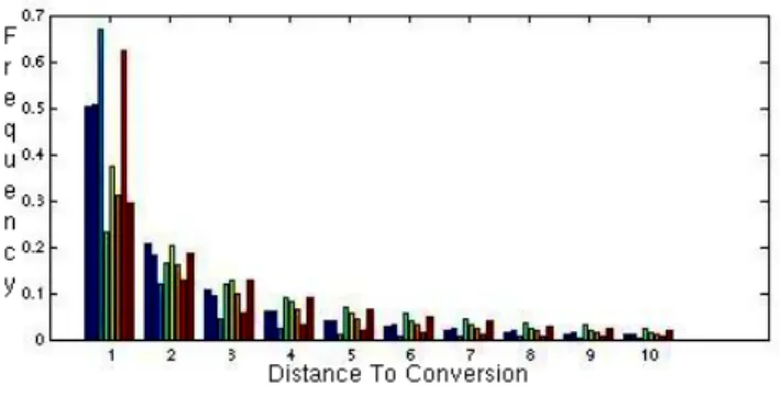
Figure 1: Distance to conversion
did not convert within the monitored time period. As the number of non-converted (yet) users is much larger than the number of converted users, we sampled from the pool of such users randomly with a sampling probability of 1%.
3.1
Descriptive Statistics
To ensure anonymity of the advertisers in our dataset, we do not report the descriptive statistics table, instead pre-senting two plots illustrating some of the most interesting properties of the data. We first ask how long (how many searches) does is take for a user to convert with the ad-vertiser (assuming that the user eventually converts)? The exact value of the statistics depends on how we average data across different users. Figure 1 shows the histogram of the distance to conversion for a randomly selectedevent in the sample of converted users. The distance is defined as the number of future ad impressions for the same advertiser (in-cluding the current impression) that this user will get before the conversion. The data on the plot is slightly distorted (by a small multiplicative random factor for every advertiser) to preserve advertiser anonymity; the distortion does not affect the main message of the plot. In about one third of the cases, the user who converts will convert immediately after the ob-served impression, however a larger fraction (2/3) will be matched to the same advertiser at least one more time before they convert. Moreover, the distribution has a heavy tail: in about 10% of the observations, the user will be matched to the same advertiser in at least 10 more searches before eventually converting. The plot also shows that there is a lot of variation across advertisers, therefore our estimates of the distance to conversion have limited generalizability outside of our sample. What we would expect to generalize is the observation thatthe interaction between the advertiser and the user is far more complex than a simple “search; click; convert” scenario and many users will be exposed to the ad-vertiser’s ad multiple times before they eventually convert.
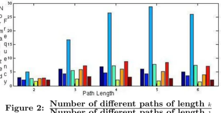
Finally, Figure 2 presents a plot showing the number of different path types of certain length in our conversion data. The path type is defined as the equivalence class of all con-version paths that are identical once the timestamps are omitted. Furthermore, we normalize all values by the num-ber of different path types of the length 1, which is essentially the number of different user queries that we observed in the conversion data. In order to understand the plot better, one can think of the two extreme cases of the data generating process. In the first scenario, the data generating process samples new events i.i.d., i.e., the queries that the user is-sued before do not affect the queries that the user will use later. In such setting, the number of different path types of the length k(assuming a very large sample size) will grow
Figure 2: Number of different paths of lengthk Number of different paths of length1 exponentially with respect to the number of possible user queries (which is often in the order of thousands or even tens of thousands for a large advertiser). This is clearly not the behavior we see in Figure 2, even taking into account finite size of our sample (we formally test the i.i.d. model in the next Section). On the other hand, a perfect correlation between user searches would imply a flat plot, which is also not the case in our sample. While there is again significant variation across advertisers, we would expect the following observation to generalize: there are strong “structural corre-lations” between user searches in a single conversion path.
4.
GENERATIVE MODELS
In this section, we formally define and evaluate a set of generative statistical models for the conversion path data. The first baseline model we evaluate is a simplei.i.d. model: every new event in a conversion path is sampled indepen-dently from everything that has happened before that. The number of parameters in the model is equal to the number of different user queries in the dataset (minus one).
All others models we evaluate represent user behavior as a random (Markov) walk in some directed graph (adgraph), what makes the models differ is the way theadgraphis con-structed. The adgraph construction involves defining the set of graph nodes V, defining the set of graph edges E, and defining the edge weights wij which represent
transi-tion probabilities between nodesiandj. While definition of the nodes in the adgraph is model-specific, all adgraphs that we construct will have three special nodes: the “begin” node representing the start of the conversion (or non-conversion) path for any user, the “conversion” node representing the conversion event and the “null” node representing the state of the users who have not converted within the observation period. The “null” node is always an absorbing node and the “conversion” node always leads to the “null” node. The “begin” node has no incoming edges.
Simple Markov. In a “Simple Markov” adgraph, every graph node is an event (impression or click) and the edge weights are just probabilities of observing the two events consecutively in a conversion path. We also consider “For-ward Markov” and “Back“For-ward Markov” adgraphs, in which we incorporate the distance from the first user observation (the distance to the last user observation) as a part of the node id, thus allowing the next event to be sampled depend-ing on how many events for the same user we have observed so far (“Forward Markov”) or how many more events we are going to observe before the user converts (“Backward Markov”).
Regime Switching Markov. We also consider three ad-ditional “Regime Switching Markov” adgraphs. In all three
Model Stab. (RMSE) Stab. (MAE)
i.i.d. 0.0000 0.0000 Simple Markov 0.1164 0.0414 Forward Markov 0.2128 0.1080 Backward Markov 0.2130 0.1068 RS Markov 1 0.1317 0.0489 RS Markov 2 0.1291 0.0475 RS Markov 3 0.1326 0.0494
Table 1: Model stability, out of sample
Model −2 LogL (Out) BIC (In) AIC (In)
i.i.d. 8.9860 9.0042 8.9714 Simple Markov 5.1155 5.2718 5.0762 Forward Markov 4.3607 4.7591 4.3229 Backward Markov 3.6291 4.0926 3.5964 RS Markov 1 4.9965 5.1797 4.9545 RS Markov 2 5.0360 5.2146 4.9949 RS Markov 3 5.0169 5.1969 4.9759
Table 2: Model fitness, in and out of sample
models, the user is assumed to have two different possible regimes: the “search” regime representing a regular browsing behavior and the “interested” regime representing the behav-ior of a user interested in a particular advertiser. Thus, for every user query we will have two different nodes: one for the “search” regime and one for the “interested” regime. The user always starts in the “search” regime and, once switched to the “interested” regime, always stays there. We consider three possible signals of the user switching the “regime”: clicking on the advertiser’s ad (“RS Markov 1”), using the advertiser’s brand name in a search query (“RS Markov 2”) or a combination of both (“RS Markov 3”).
We have evaluated all seven models in terms of several criteria: average stability (sampling variance) of the edge weights in the constructed graph (parameter estimates for the i.i.d. model) and fitness both in and out of sample. Stability scores were calculated in two forms: the average (across all edges) root mean squared error (RMSE) and the mean absolute error (MAE) of the edge weight estimates in a five sample split of the data. Table 1 shows that, with exception of the i.i.d. model, the edge weight estimates are quite volatile in our dataset, due to the fact that we have limited number of observations for many node pairs.6 As the next Section shows, this in fact is not a problem for stability of the corresponding adfactors.
Next, we present the fitness results for all models in Ta-ble 2. We report the statistical model fit to the data in-sample as measured by the Akaike Information Criterion (AIC) and the Bayesian Information Criterion (BIC) [3]. We also report the out of sample fit from five-fold cross-validation [19] using the log-likelihood as the fitness crite-ria. As expected, the i.i.d. model shows the worst fit by far. The best fitting model according to all three criteria is the “Backward Markov” model, indicating that the distribution of queries issued by the user varies significantly with the dis-tance from the conversion event. Regime switching models fit slightly better than the “Simple Markov” model.
5.
AD FACTORS
In this section, we define and evaluate a number of ad-factors that capture structural correlations in the conver-sion path data. All adfactors are calculated directly on the graph structures we defined in the previous section, for in-stance, the same adfactor can be calculated both for a “Sim-6
While the i.i.d. model is stable, it provides bad fit to the data as shown in Table 2. This is just another example of the classic bias-variance tradeoff.
ple Markov” adgraph as well as for a regime switching ad-graph. We present several alternative versions of the adfac-tors and evaluate their properties on the actual data. The adfactor is calculated for every node in the adgraph and, informally, can be thought of as a measure of structural cor-relation between this node and the target node (the conver-sion node). The simplest adfactor would be a simple edge weight between the pair of nodes in the adgraph. Such ad-factor would capture a simple correlation between a pair of consecutive events: how often do users who get an ad im-pression for a particular query click on it? (clickthrough rate) how often do users who click on the ad convert with the advertiser? (conversion rate) The more sophisticated adfactors we define are expected to capture the structural properties of the adgraph such as: ceteris paribus, the larger the number of the disjoint paths from an event to the con-version is, the higher the adfactor should be, and also, the closer these events are, the higher the adfactor should be.
Three important points should be made about the adfac-tors. First, while we expect the adfactors to have useful applications (and we show some of the applications in this paper) and be useful for ranking and reporting purposes, we do not and cannot attach any causal meaning to the val-ues. What adfactors capture are correlations not causations. This is even true for the simplest of the currently used mod-els of ad performance such as the conversion rate; what the conversion rate says is what fraction of the users converted with the advertiser after clicking on an ad, not what frac-tion of the users converted with the advertiser because of the ad (some users would have converted anyway even if the ad was not shown; other users who did not convert immediately may have converted later because of the ad). Establishing causation would require running an actual experiment or, at least, having a good exogenous source of randomness in the data; this is beyond the scope of the paper.
Second, there is no ex-ante measure of quality of an adfac-tor and we are not going to say that one adfacadfac-tor is always better than another. What we will say in the rest of the paper is what structural properties of the data the differ-ent adfactors are able to capture. Third, in order for the adfactors to be practically useful, they should be efficiently computable on large-scale data sets. To address this issue, we design efficient algorithms for all adfactors we introduce in this paper, using distributed computation paradigm. In fact, for one of the adfactors (the PPR adfactor), we can directly use a local pushback algorithm developed by Ander-sen et. al [4]. For the rest of adfactors, we preAnder-sent suitable adaptations of the pushback algorithm.
5.1
LastAd
LastAd adfactor represents the conversion rate of the cor-responding ad: it measures the weight of the direct edge from the corresponding node to the conversion node. For-mally, for any event e (either simple ad impression or ad click), the LastAd adfactor is
lastad(e) = number of occurrences of{e, conversion} number of occurrences ofe
5.2
PageRank contribution (PPR, CPR)
PageRank contribution adfactor is defined as the Person-alized PageRank contribution of the evaluated node v to the conversion nodec (ppr(v, c)). Below, we give a formal definition.
Assume some restart probabilityα >0 and a graph given by the n×n random walk matrix M (M(i, j) = wij
P
kwik). Let I be the identity matrix and ev is the row unit vector whosev-th entry is equal to one.
The Personalized PageRank matrix is defined as anbyn matrix solution of the following equation
pprα=αI+ (1−α) pprαM.
Fix a nodev. Thev-th row of the matrix satisfies pprα(v,·) =αev+ (1−α) pprα(v,·)M.
This is known as the Personalized PageRank (PPR) vector of a nodevwith restart probabilityαand it was introduced by Haveliwala [15] as the stationary distribution of a random walk on the graph withαprobability restart at nodevafter each step.
The dual construct to the PPR vector is obtained by tak-ing a stak-inglecolumn of the matrix. The column correspond-ing to the conversion nodec, consists of all PPR contribu-tions for different nodes vand the fixed conversion node c and, when written in a row form, solves the following equa-tion
pprα(·, c) =αec+ (1−α) pprα(·, c)MT.
This is PageRank contribution (CPR) vector and it is de-noted as cpr ≡ pprα(·, c) [4]. The CPR vector naturally
captures important structural properties of the graph such as the number of different paths from every nodev to the conversion nodec as well as the lengths of these paths. A nice property of cpr is that the sum of all cpr’s for the nodec is equal to the PageRank of the nodec, so it can be thought of as a way to divide the PageRank score (which captures the total credit of the conversion node in the graph) into con-tributions from other nodes. Moreover, varying the restart probability of the random walk (α) can be used to fine-tune the trade-off between the short-term and the long-term ef-fects of the ads. The higher the restart probability is, the more the score captures the short-term contribution of the ad as compared to the long-term one.
5.3
Eventual Conversion
Theeventual conversionadfactor isa limiting case ofcpr
when the restart probabilityαconverges to zero. The follow-ing proposition says that, after normalization, this adfactor is equivalent to the probability of hitting the conversion node as opposed to hitting the null node in a random walk with no restart. This adfactor is denoted hit(·, c).
Proposition 1. Let Mˆ be the random walk matrix with the “null” node excluded and assume that the matrixI−Mˆ is
invertible, whereI is the identity matrix.7 Define the “hit” vectorhit(·, c)as a row vector solving the following equation:
hit(·, c) = hit(·, c) ˆMT+ec. Then, lim α→0 ∂pprα(·, c) ∂α = limα→0 pprα(·, c) α = hit(·, c). 7
A sufficient but not necessary condition for this is that every node except for the “null” node has a small probability of transition to “null”. This is a reasonable assumption for our application as the user can always “drop out” with some positive probability.
5.4
Visit
For comparison purposes, we define the visit adfactor which represents the random walk (no restart) visit probability of a node from the “begin” node. This adfactor is not related to the conversion node but simply captures the likelihood of the event happening in a user conversion path. Formally, the adfactor is defined as a row vector hit(b,·) solving
hit(b,·) = hit(b,·) ˆM+eb.
Similar to Propositon 1, one can show that lim
α→0
∂pprα(b,·)
∂α = hit(b,·).
5.5
Marginal Increase (Passthrough)
We introduce the MIα(j) adfactor, which represents the
marginal increase in the probability of hitting conversion from the “begin” nodebif we increase the weight of all edges outgoing from the nodejbyε, allocated in proportion to the current edge weights. We first compute MIα(j) in the
con-text of Personalized PageRank with a restart probabilityα. Let ∂pprα(b,c)
∂wji be the marginal influence of an edge weight wjion the PPR of the “begin” node for the conversion node.
The adfactor MIα(j) can be proxied by the following
sum-mation (note that sensitivity with respect to each outgoing edge is weighted proportionally to the current edge weight).
MIα(j) = X i wji ∂pprα(b, c) ∂wji ,
We first observe that, in the setting of random walks with restartα, ∂pprα(b,c)
∂wij can be computed by using the following Proposition:
Proposition 2. The marginal influence of an edge weight on the PPR of the sinkcwith restart at the source nodebis given by a product of the PPR of the start node of the edge (i) with restart at the source nodeband the PPR of the sink nodecwith restart at the end node of the edge (j):
∂pprα(b, c) ∂wij
= 1−α
α pprα(b, i) pprα(j, c).
Using this proposition, we derive a simple closed-form for-mula for MIα(j).
Proposition 3. The marginal effect of increasing the weight of the outgoing edges of a nodej, MIα(j), is equal to:
MIα(j) =
pprα(b, j) pprα(j, c)
α . (1)
The proofs are left to the appendix. An advantage of this closed-form formula is that it lets us apply fast algorithms for computing the MIα adfactor. The above proposition
also implies that, asαtends to zero, the MI adfactor can be computed as follows:
Proposition 4. The marginal effect of increasing the weight of the outgoing edges from a nodejon the hitting probability of conversion, MI(j), is equal to:
MI(j) = lim
α→0
MIα(j)
α = hit(b, j) hit(j, c). (2)
Table 3: Correlation matrix for adfactors. α= 0.05
PPR Ev.Conv. LastAd Visit Pass
PPR 1.0000 0.9733 0.7285 -0.0657 0.1321
Ev.Conv. 0.9733 1.0000 0.7064 -0.0614 0.1370
LastAd 0.7285 0.7064 1.0000 -0.0542 0.0991
Visit -0.0657 -0.0614 -0.0542 1.0000 0.8006
Pass 0.1321 0.1370 0.0991 0.8006 1.0000
The above observation implies that the MI adfactor is the same as thepassthroughadfactor which isthe change in
hit(b, c)if we remove the nodejfrom the graph and redirect all incoming edges to this node to the “null” node, or formally,
Pass(i) = hit(b, i) hit(i, c).
We call the corresponding adfactor the “passthrough” or Pass adfactor, since it captures the value of random walks passing through the evaluated node.
5.6
The Removal Effect
In this part, we introduce the adfactor RE(i) for each node iwhich is defined asthe change in the probability of hitting conversion starting from the “begin” nodebif we re-move node ifrom the graph. Intuitively, this adfactor cap-tures the change in the probability of reaching conversion if we remove a nodei, or the incoming edges of nodei. Simi-lar to the MIα adfactor, we define the REα adfactor in the
context of a random walk with restart probabilityαas REα(i) = X j wji ∂pprα(b, c) ∂wji ,
Using Proposition 2, we can derive a similar closed-form formula for RE(i) which is shown to be equal to Pass(i).
Proposition 5. The REαand RE adfactors can be
com-puted as follows: REα(i) = pprα(b, i) pprα(i, c) α . (3) RE(i) = lim α→0 REα(i) α = hit(b, i) hit(i, c). (4) The proofs are left to the appendix. The Pass adfactor is a proxy for both MI and RE adfactors, i.e., MI(i) = RE(i) = Pass(i). As a result, we only report empirical results for the passthrough (Pass) adfactor, and this will imply the same results for the MI and RE adfactors.
5.7
Efficient Algorithms
Computational efficiency is crucial for successful applica-tion of any data mining algorithm to the real world advertis-ing data. Fortunately, all adfactors introduced in the previ-ous Section can be efficiently computed on large scale graphs using parallel machines. The key is the observation that the PageRank contribution vectors (cpr≡ppr(·, c)) can be effi-ciently computed using a local algorithm which adaptively examines only a small portion of the input graph near a spec-ified vertex [4]. We have implemented the algorithm of [4] in the distributed computing environment of MapReduce [11] using the Pregel framework [21]. In the Pregel framework, every node in the graph can perform its local computation and the nodes interact with each other by a periodic ex-change of messages. The cpr computation can be achieved by a simple local algorithm (Algorithm 1), in which every node has state consisting of two variables: the currently ac-cumulated cpr and the residual value obtained from other
nodes but not yet distributed(resid). The nodes run a simple pushback operation (pushing fraction of the residual to its neighbors over incoming edges) until the value of the resid-ual in each node does not exceedε. Andersen et al [4] proves the following:
Theorem 1. [4] The following algorithm calculates anε -approximation of the PageRank contribution vector for the conversion node, i.e. cpr ≡ ppr(·, c), using only 1
αε + 1
pushback operations. Moreover, using this algorithm, one can identify the top k nodes with the maximum PageRank contribution using onlyO(k
α) pushback operations.
Algorithm 1Local algorithm to calculate cpr ≡ppr(·, c) adfactor of the conversion nodec.
Initialization:
cpr(u)⇐0, resid(u)⇐1 if conversion node otherwise 0 Main Loop:
while∃usuch that|resid(u)| ≥εdo Pushback(u, α)
end while Pushback (u, α):
cpr(u)⇐cpr(u) +αresid(u){accumulateαfraction of the current residual}
forevery incoming edgew−→udo
resid(w)⇐resid(w) + (1−α)doutresid(u)(w) {distribute 1−αfraction of the current residual to neighbors}
end for resid(u)⇐0
Using Propositions 3 and 5, one can see that calcula-tion of the MIαand REα, and passthrough (Pass) adfactors
requires estimating both the Pagerank contribution vector for conversion (i.e, the ppr(·, c) value for every node in the graph) and the Personalized PageRank vector of the begin node (the ppr(b,·) value for every node in the graph). The ε-approximation of the Pagerank contribution vector can be calculated efficiently using pushback operations in Algo-rithm 1. Moreover, a similar pushforward algoAlgo-rithm devel-oped in [17] can be used for calculation of theε-approximation of the PPR vector for the begin node. Using Propositions 3, 4, and 5, by multiplying these two vectors, we get the following theorem:
Theorem 2. There exists a local ε-approximation algo-rithm for computing the MIα and REα using O
` 1
αε
´
push operations. Moreover, anε-approximation for Pass, MI, and RE can be computed usingO` 1
α0ε
´
whereα0= miniwi,null.
6.
EMPIRICAL PROPERTIES OF
ADFAC-TORS
In this section, we present some interesting empirical prop-erties of the adfactors in our dataset. All experiments were done with the “Simple Markov” graph, except where explic-itly specified otherwise. The primary reason we chose “Sim-ple Markov” over other adgraph models is that it simplifies interpretation of the results. While similar experiments can be performed with other adgraphs, the results and their in-terpretation would be different for every particular adgraph model used.
Table 3 presents correlations between different adfactors in our data. As expected, for a sufficiently small value of the restart probability (α = 0.05), the PageRank contribution adfactor is highly (ρ = 0.9773) correlated to the Eventual Conversion (hit(·, c)) adfactor. There is also a significant
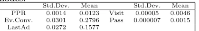
Table 4: Stability of the adfactors for the top 1000 nodes.
Std.Dev. Mean Std.Dev. Mean
PPR 0.0014 0.0123 Visit 0.00005 0.0046
Ev.Conv. 0.0301 0.2796 Pass 0.000007 0.0015
LastAd 0.0272 0.1577
but much lower correlation between the PPR factor and the Last Ad adfactor (ρ= 0.7285). The visit adfactor is almost uncorrelated to the PPR, eventual conversion and the Last Ad adfactors, indicating that the user queries that occur fre-quently are not necessarily well connected to the conversion event. Since the passthrough adfactor incorporates the visit adfactor, it is also weakly correlated to the rest of the ad-factors. All correlations are statistically significant at 1% level.
Table 4 shows stability results (the sample standard de-viation) for the adfactors of the top 1,000 graph nodes in a five-fold sample split. One can see that the standard devia-tions of all adfactors are relatively low compared to the mean values suggesting that the adfactors of the most important nodes in the graph are relatively stable in the presence of sampling variance even though the edge weights in the graph can be volatile (Table 1).
In the rest of this Section, we evaluate how adfactors corre-late with other node attributes such as brand/non-brand8, click/impression and broad/exact match. Note that in all three cases the evaluated attribute is a binary variable, thus, instead of presenting simple correlations, one can deliver better intuition by using ROC curves for the correspond-ing classifier. Consider, for instance, Figure 3. For every adfactor, one can construct a classifier of node “brand-iness” by using the adfactor < T decision rule: if the adfactor is larger than the threshold T, classify it as brand (or non-brand depending on which one is better), otherwise classify it as nonbrand (brand). Varying values ofT, one can achieve different (precision, recall) points; all such points constitute the ROC curve.
Figure 3 shows that the PPR adfactor is an excellent pre-dictor of “brand-iness” for impressions (AUC = 0.95509), even stronger than the last ad score (AUC = 0.89930). At the same time, for clicks the conversion Pass adfactor gives the best predictor of the brand (AUC = 0.87707), although it is an extremely weak predictor for impressions (AUC = 0.57120). We suggest that users who search with brand queries are (naturally) much more likely to convert with the advertiser, than users that search with generic queries, thus the PPR adfactor measuring structural correlation to the conversion event is a good signal of the brand nature of the user query. Yet, once the user clicks on the adver-tiser’s ad, the signal loses its value, because, once the ad attracted enough user attention, the query that triggered the ad in the first place becomes much less important. The good predictive power of the Pass adfactor on click but not impression “brand-iness” suggests that users are more likely to convert with the advertiser through click on a brand query ad rather than through click on a non-brand query ad, how-ever converting users get equal exposure to both brand and non-brand impressions before they convert.
8
Queries were marked asbrandif they included a phrase with the edit distance of at most three to the advertiser’s name or the brand name, and marked as non-brandotherwise. The results were manually inspected to ensure that the mapping is reasonable.
Figure 3: ROC curve for brand prediction for clicks (top) and impressions (bottom)
Figure 4: ROC curve for click prediction for brand queries (top) and nonbrand queries (bottom)
Figure 4 shows that for brand queries the Last Ad adfac-tor and the PPR adfacadfac-tor are excellent signals of the click attribute; for non-brand queries they predict well for recall of up to approximately 0.6, after which the precision-recall curve becomes flat (until the eventual jump to (1.0,1.0)). This weird behavior can be attributed to the fact that, in our dataset, we observe a number of rare generic (non-brand specific) queries, for which click on the ad does not lead to any conversion. We emphasize that such queries are rare, therefore using the Pass adfactor filters them out and the Pass adfactor shows excellent predictive power for the non-brand queries in Figure 4.
Next, we compare the PPR and the Last Ad adfactors by using a difference between the ad rank in both models as a predictor for brand/non-brand, click/impression and
Figure 5: ROC curve for (PPR rank - last ad rank) predictor
Figure 6: PPR behavior as a function of distance to conversion
Figure 7: ROC curve for brand prediction by differ-ent models
broad/exact attributes. Results in Figure 5 suggest that the difference is a good predictor of the brand attribute; manual inspection shows that this is because the PPR factor ranks brand nodes even higher than the Last Ad ad-factor. On the other hand, the ROC curves for click and phrase(broad)/exact match prediction are close to diagonal suggesting that there is no systematic difference in rankings of clicks/impressions and broad/exact match nodes by both methods.
Next, we plot the PPR behavior as a function of the dis-tance to conversion in Figure 6. The figure was constructed using the data from the “Backward Markov” model, in which every user query is represented by multiple nodes in the graph, depending on its distance from the conversion node. Thus, for every queryq, one can calculate
log (ppr(qat distanced, c))−log (ppr(qat distance 1, c)) 9. Figure 6 shows average of these results for different groups. Note that for clicks the PPR values at distance two and more from conversion are significantly smaller than the PPR val-ues at distance one, suggesting that if the user clicks on the ad and does not convert immediately, the likelihood to con-vert in the future goes down. Consistent with our prior ob-servations, the PPR behavior for brand and non-brand clicks is similar. On the other hand, for non-brand impressions the PPR grows (or at least doesn’t decrease) with distance to conversion, indicating that exposure to the advertiser ad on non-brand queries can have a long-term positive correlation with the likelihood of the user to convert. For brand im-pressions, the PPR decreases with distance to conversion, although not as strongly as for clicks, again suggesting that, if the user searches for a brand and does not convert soon enough, the likelihood of converting in the future goes down. Finally, Figure 7 investigates how different graph struc-tures affect the relationship between the PPR adfactor and the brand attribute of the node. We consider three models: “Simple Markov”, “Backward Markov” and “RS Markov 1”. 9The log representation was primarily chosen to reduce sen-sitivity to outliers.
For “Simple Markov” model we simply plot the ROC curve using the PPR adfactor as a predictor for brand. For “Back-ward Markov” model we use the observation (from Figure 6) that the PPR of brand nodes decays with distance from con-version while the PPR of nonbrand nodes grows with dis-tance from conversion, thus we use
10
X
d=2
(log (ppr(qat distanced, c))−log (ppr(qat distance 1, c))) as the predictor. For the “RS Markov 1” model, we would expect similar behavior to hold and the PPR of the brand nodes in the “search” state (before the user clicked on any ads) to be lower than that in the “interested” state (after the user clicked on some ad), while the PPR of the nonbrand nodes in the “interested” state to be higher than that is the “search” state; thus, we construct the predictor as
log (ppr(q in search state, c))−log (ppr(qin interested state, c)). Figure 7 shows that the “RS Markov 1” model has the best predictive power for the brand attribute, confirming the in-tuition that user clicks have different value in brand and non-brand contexts.
7.
DATA MINING TOOLS
Producing intuitive and concise reports from huge amounts of data is the desired goal for advertisers. In this section, we discuss various data mining tools that can be developed using our ad factors defined on the graph models introduced in the paper.
Identifying the topk ads with the largest adfactor.
The simplest type of report one can think of is identifying the topkads with the largest adfactors in a particular graph model. The value of such report depends on the particular adfactor and the underlying graph model used. For instance, in Section 6, we show that the PPR adfactor (in the “Simple Markov” graph) has high but not perfect correlation with the brand attribute of the ad impression. Identifying the topk impressions with the PPR adfactor can thus be interpreted as identifying the topk impressions (user queries) with the highest “branding” impact: many of these user queries will in fact have the advertiser name or the brand name in them, but some will not and thus can be thought of as “shadow brands”. Due to privacy issues, we cannot show an actual example of such output. Another interesting example of the topkoutput is the topkimpressions for the Pass adfactor; they can be thought of as the topkuser queries associated with the largest revenue to the advertiser if one takes into account the long-term correlations in the graph. Interest-ingly, from Figure 3, we know that these are uncorrelated with the brand attribute.
Identifying ads with significant long-term effects not taken into account by the Last Ad model.
Advertisers traditionally rely on the Last Ad reports (click-through and conversion rates) to evaluate ad effectiveness. An alternative report we suggest would be to look for ads that are ranked higher with adfactors taking into account the long-term correlations (like PPR) than with the Last Ad adfactor. One such criteria for ranking is the difference be-tween the PPR adfactor node rank and the Last Ad adfactor node rank (properties of this criteria are shown in Figure 5). Another criteria is to look for impressions that either have
the PPR growing with the distance from conversion (“Back-ward Markov” model) or have the PPR in the “search” state higher than in the “interested” state (“RS Markov 1” model). As Figure 7 shows, the second approach is more biased to-wards the brand impressions than the first one.
Identifying the topkads with the maximum marginal increase (MI) adfactor.
A popular advertising objective is to maximize the expected number of user conversions given a certain budget constraint. In a random walk model, we can restate it as maximizing the probability of hitting the conversion node starting from the “begin” node. A heuristic way to identify the valuable nodes to invest on is to examine a small increase on the bid of a query (or keyword) which will have the maximum ef-fect on the probability of hitting the conversion node. This small increase on the bid results in a small increase in the weight of incoming edges for this query. Thus, in order to identify queries for which the increase in their bid results in the maximum marginal increase in the probability of hitting conversion, we can look for the topkads with the maximum MI adfactor, and the advertiser may consider increasing the bid for queries with large MI.10
Explaining the adfactor value
The adfactor assigned to any particular node in the graph, must be easily explained by a local structure around this node. For instance, for the PPR (PageRank contribution) adfactor of a node u, one can always consider the top-m neighbor nodes through which the explained node u tributes the largest fraction of the PageRank to the con-version node. Formally, let πu be the permutation of all
neighbors of the nodeuthat arranges them in the decreas-ing order ofwuvpprα(v, c). We defineπu(m) as the set of
the first mnodes in the permutation. These nodes can be thought of as the most likely next actions of the user after the explained action, assuming that the user is going to convert. It is straightforward to extend the pushback Algorithm 1 to keep track of the topmcontributors for every node, thus one can efficiently generate corresponding reports. The reports are best represented as graph plots, constructed starting at a seed nodesand going up to a distancedin a graph of the top-mneighbors of every node. Due to privacy reasons as well as the space limit, we omit an example of such plot.
8.
CONCLUSIONS
Online advertisers have access to aggregate statistics such as the clickthrough rate, the conversion rate or the lift of their ad campaigns, but seek to understand more sophisti-cated correlations in users’ trajectories of ads seen and users’ actions. Here we introduce an alternative data mining tech-nique for aggregating user-level advertising data. We define various adgraphs to model the data pertinent to the ad-vertiser and propose several adfactors based on stationary probabilities of suitable random walks to quantify the im-pact of ad events. We show anecdotal evidence for adfactors and describe their potential data mining applications.
Our research introduces novel primitives for mining advertiser-specific data for ad effects. Adfactors we define are succinct, easy to compute and capture many structural properties of 10We emphasize that this is only a heuristic. Any practical bidding strategy should also take into account the current bidding landscape (how much do the advertiser and the com-petitors bid) for a particular keyword.
users’ trajectories. In the future, richer data mining prim-itives can be developed using adfactors, which may poten-tially reveal more sophisticated correlations in user behav-ior, including negative correlations. Other valuable direc-tions for future research include developing richer graphical models of user behavior, beyond the Markov models in this paper, and adapting adfactors to them.
Acknowledgements. We would like to thank Chao Cai, Zhimin He, and Sissie Hsiao for helping us with the data sets, and Sheng Ma, Fernando Pereira, R. Srikant for interesting discussions.
9.
REFERENCES
[1] E. Agichtein, E. Brill, and S. Dumais. Improving web search ranking by incorporating user behavior information. InSIGIR ’06: Proceedings of the 29th annual international ACM SIGIR conference on Research and development in information retrieval, pages 19–26, 2006.
[2] R. Agrawal and R. Srikant. Fast algorithms for mining association rules. InProceedings of the 20th International Conference on Very Large Databases (VLDB’94), pages 487–499, 1994.
[3] H. Akaike. A new look at the statistical model identi↓cation.IEEE Transactions on Automatic Control, 19:716– 723, Dec 1974.
[4] R. Andersen, C. Borgs, J. Chayes, J. Hopcroft, V. Mirrokni, and S.-H. Teng. Local computation of pagerank contributions.Internet Mathematics, 5:23–45, Jan. 2009.
[5] Atlas. Engagement mapping. Thought Paper, Available at
http://www.atlassolutions.com/uploadedFiles/Atlas/Atlas\_Institute/Engagement\ _Mapping/eMapping- TP.pdf, 2008.
[6] S. Baluja, R. Seth, D. Sivakumar, Y. Jing, J. Yagnik, S. Kumar, D. Ravichandran, and M. Aly. Video suggestion and discovery for youtube: taking random walks through the view graph. InProceedings of the 17th International Conference on World Wide Web, WWW, pages 895–904, 2008. [7] H. Cao, D. Jiang, J. Pei, E. Chen, and H. Li. Towards context-aware
search by learning a very large variable length hidden markov model from search logs. InWWW ’09: Proceedings of the 18th international conference on World wide web, pages 191–200, 2009.
[8] comScore. Whither the click? comscore brand metrix norms prove ‘view-thru’ value of on-line advertising. Available at
http://www.comscore.com/press/release.asp?press=2587, 2008. [9] G. Cormode, F. Korn, S. Muthukrishnan, and Y. Wu. On signatures for
communication graphs. InProceedings of the 24th International Conference on Data Engineering, ICDE, pages 189–198, 2008.
[10] E. E. Dar, Y. Mansour, V. Mirrokni, S. Muthukrishnan, and U. Nadav. Budget optimization for broad-match ad auctions. InWWW, World Wide Web Conference, 2009.
[11] J. Dean and S. Ghemawat. Mapreduce: simpli↓ed data processing on large clusters.Communications of ACM, 51(1):107–113, 2008.
[12] T. Fawcett and F. J. Provost. Combining data mining and machine learning for e↑ective user pro↓ling. InProceedings of the Second International Conference on Knowledge Discovery and Data Mining (KDD), pages 8–13, 1996. [13] J. Feldman, S. Muthukrishnan, M. Pal, and C. Stein. Budget optimization
in search-based advertising auctions. InEC ’07: Proceedings of the 8th ACM conference on Electronic commerce, pages 40–49, 2007.
[14] A. Hassan, R. Jones, and K. Klinkner. Beyond DCG: User behavior as a predictor of a successful search. InWSDM ’10: Proceedings of the 3rd international conference on web search and data mining, 2010. Forthcoming. [15] T. H. Haveliwala. Topic-sensitive pagerank: A context-sensitive ranking
algorithm for web search.IEEE Transactions on Knowledge and Data Engineering, 15(4):784–796, 2003.
[16] A. Inokuchi, T. Washio, and H. Motoda. An apriori-based algorithm for mining frequent substructures from graph data. InPrinciples of Data Mining and Knowledge Discovery, pages 13–23, 2000.
[17] G. Jeh and J. Widom. Scaling personalized web search. InWWW ’03: Proceedings of the 12th international conference on World Wide Web, pages 271–279, 2003.
[18] K. Keller. Brand equity and integrated communication. InIntegrated Communication: Synergy of Persuasive Voices, 1996.
[19] R. Kohavi. A study of cross-validation and bootstrap for accuracy estimation and model selection. InProceedings of the Fourteenth International Joint Conference on Artificial Intelligence, pages 1137–1145, 1995.
[20] R. Lewis and D. Reiley. Retail advertising works!: Measuring the e↑ects of advertising on sales via a controlled experiment on yahoo! Working paper, Yahoo! Research, 2009.
[21] G. Malewicz, M. H. Austern, A. J. Bik, J. C. Dehnert, I. Horn, N. Leiser, and G. Czajkowski. Pregel: a system for large-scale graph processing. In
PODC ’09: Proceedings of the 28th ACM symposium on Principles of distributed computing, pages 6–6, 2009.
[22] H. Mannila, H. Toivonen, and I. Verkamo. Discovery of frequent episodes in event sequences.Data Mining and Knowledge Discovery, 1:259–289, Sept. 1997.
[23] S. Muthukrishnan, M. Pal, and Z. Svitkina. Stochastic models for budget optimization in search-based advertising. InLecture Notes in Computer Science, Internet and Network Economics, pages 131–142, 2007.
[24] L. Page, S. Brin, R. Motwani, and T. Winograd. The pagerank citation ranking: Bringing order to the web. Technical Report. Stanford InfoLab., 1999.
[25] K. Sugiyama, K. Hatano, and M. Yoshikawa. Adaptive web search based on user pro↓le constructed without any e↑ort from users. InWWW ’04: Proceedings of the 13th international conference on World Wide Web, pages 675–684, 2004.
10.
APPENDIX
Proof of Proposition 1 Proof. From [4] pprα(·, v) =αev ∞ X t=0 (1−α)t(MT)t.After taking the derivative ∂pprα(·, c) ∂α =pprα(·, c) α +αec ∞ X t=1 t(1−α)t−1(MT)t.
It immediately follows that
‚ ‚ ‚ ‚ ‚ ∂pprα(·, c) ∂α −pprα(·, c) α ‚ ‚ ‚ ‚ ‚∞ →0.
Next, we haveh=ec+hM Tand
pprα(·, c) =αec+ (1−α) pprα(·, c)MT, which is equivalent to pprα(·, c) α =ec+ 1−α α pprα( ·, c)MT. After substraction h−pprα(·, c) α = h −1−α α pprα( ·, c) ! MT, or h−pprα(·, c) α ! = pprα(·, c)MT“I−MT”−1→0, as pprα(·, c)→0. Proof of Proposition 2
Proof. We know that the ppr vectorpwith restart at nodebsolves the equa-tionp=αeb+ (1−α)pM, whereMis the transition matrix. Fix nodesiandj and take a derivative with respect towij:
∂p ∂wij = (1−α)p∂M ∂wij + (1−α) ∂p ∂wij M. Now, ∂M
∂wij is a zero matrix with a single 1 at rowiand columnj. It follows that ∂p ∂wij = (1−α)p[i]ej+ (1−α) ∂p ∂wij M,
wherep[i] is thei-th component of the vectorp. This can be written as ∂p ∂wij = 1−α α p[i] ! αej+ (1−α) ∂p ∂wij M,
and by linearity of the PPR we can see that this is just“1−ααp[i]”times the PPR vector with restart at nodej, i.e.,
∂pprα(b, c) ∂wij
=1−α α
pprα(b, i) pprα(j, c).
Proofs of Propositions 3 and 5
Proof. For outgoing edges, we can use the equality pprα(i, c) =αI(i == c) + (1−α) pprα(j, c)wij[4], as shown below:
X j wij∂pprα(b, c) ∂wij = (1−α) pprα(b, i) α 0 @ X j wijpprα(j, c) 1 A = 1−α α pprα(b, i) 1 1−α pprα(i, c) = pprα(b, i) pprα(i, c) α .
For incoming edges, we can use similar trick with pprα(b, i) =αI(i==b) + (1−
α) pprα(b, j)wji.
Proof of Theorem 2
Proof. M IαandREαcan be approximated by Theorem 1 of [4]. For MI, RE and Pass simply note thatMˆ can be written as (1−α0)M∗, whereM∗is a valid random walk matrix (every row sums to at most 1.0, the rest goes to “null”). One can therefore calculate hit and all derivative adfactors (MI, RE and Pass) via a pushback algorithm for the PPR of a random walk with the restart probabilityα0so Theorem 1 of [4] works again.