Swarm-based Algorithms for Neural Network Training

(1)

Network Training

Reginald McLean

Submitted in partial fulfilment

of the requirements for the degree of

Master of Science

Department of Computer Science

Brock University

St. Catharines, Ontario

c

(2)

Abstract

The main focus of this thesis is to compare the ability of various swarm intelligence algorithms when applied to the training of artificial neural networks. In order to compare the performance of the selected swarm intelligence algorithms both classifi-cation and regression datasets were chosen from the UCI Machine Learning reposi-tory. Swarm intelligence algorithms are compared in terms of training loss, training accuracy, testing loss, testing accuracy, hidden unit saturation, and overfitting.

Our observations showed that Particle Swarm Optimization (PSO) was the best performing algorithm in terms of Training loss and Training accuracy. However, it was also found that the performance of PSO dropped considerably when examining the testing loss and testing accuracy results. For the classification problems, it was found that firefly algorithm, ant colony optimization, and fish school search outperformed PSO for testing loss and testing accuracy. It was also observed that ant colony optimization was the algorithm that performed the best in terms of hidden unit saturation.

(3)

To my parents for their unconditional love and support throughout my education and my future endeavours. To my sister for always being willing to read about many Computer Science topics that she does not fully comprehend. To my partner for her constant love and support through many long stressful nights. Lastly, to Prof. Ombuki-Berman and Prof. Engelbrecht for their support, guidance, and extensive expertise in the field that allowed me to complete this work.

(4)

5.3 Experimental Parameters . . . 42 6 Results 44 6.1 Regression Results . . . 45 6.2 Classification Results . . . 45 6.3 Overall Results . . . 46 6.4 Saturation Results . . . 52 6.5 Overfitting Results . . . 55 7 Conclusion 58 7.1 Performance of SI Algorithms . . . 58 7.2 Future Work . . . 59 Bibliography 66 Appendices 67 A Additional Experimental Analysis 67 A.1 Parameters . . . 67

(6)

List of Tables

5.1 Neural Network Architectures for each Dataset . . . 40

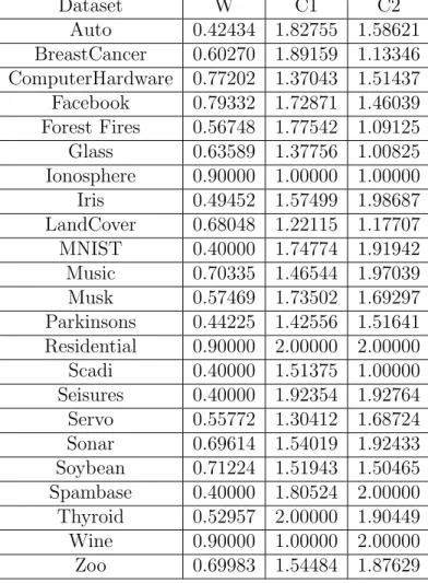
5.2 PSO with Tanh Activation function parameters . . . 43

6.1 Testing Loss Regression Datasets . . . 46

6.2 Testing Loss Classification Datasets . . . 47

6.3 Testing Accuracy Classification Datasets . . . 48

6.4 Testing Loss Overall Results . . . 49

6.5 Testing Loss Small Dataset Ranks . . . 50

6.6 Testing Loss Medium Dataset Ranks . . . 50

6.7 Testing Loss Large Dataset Ranks . . . 50

6.8 Testing Accuracy Small Dataset Ranks . . . 51

6.9 Testing Accuracy Medium Dataset Ranks . . . 51

6.10 Testing Accuracy Large Dataset Ranks . . . 51

6.11 Saturation Rankings for Regression Datasets . . . 52

6.12 Saturation Results for Classification Datasets . . . 53

6.13 Saturation Results . . . 54

6.14 ACO Saturation Results Compared to Training and Testing Loss . . . 55

6.15 Overfitting Results . . . 57

A.1 PSO with Sigmoid Activation function . . . 68

A.2 PSO with Elliot Activation function . . . 69

A.3 PSO with Lecun Activation function . . . 70

A.4 ABC with Tanh Activation function . . . 71

A.5 ABC with Sigmoid Activation function . . . 72

A.6 ABC with Elliot Activation function . . . 73

A.7 ABC with Lecun Activation function . . . 74

A.8 ACO with Tanh Activation function parameters . . . 75

A.9 ACO with Sigmoid Activation function Parameters . . . 76

(7)

A.12 BA with Tanh Activation function parameters . . . 79

A.13 BA with Sigmoid Activation function parameters . . . 80

A.14 BA with Elliot Activation function parameters . . . 81

A.15 BA with Lecun Activation function parameters . . . 82

A.16 BFA with Tanh Activation function parameters . . . 83

A.17 BFA with Sigmoid Activation function parameters . . . 84

A.18 BFA with Elliot Activation function parameters . . . 85

A.19 BFA with Lecun Activation function parameters . . . 86

A.20 FSS with Tanh Activation function parameters . . . 87

A.21 FSS with Sigmoid Activation function parameters . . . 88

A.22 FSS with Elliot Activation function parameters . . . 89

A.23 FSS with Lecun Activation function parameters . . . 90

A.24 Firefly with Tanh Activation function parameters . . . 91

A.25 Firefly with Sigmoid Activation function parameters . . . 92

A.26 Firefly with Elliot Activation function parameters . . . 93

A.27 Firefly with Lecun Activation function parameters . . . 94

A.28 Training Loss Results . . . 95

A.32 Training Accuracy Results . . . 99

A.36 Testing Loss Results . . . 101

A.40 Testing Accuracy Results . . . 105

A.44 Saturation Results . . . 107

(8)

A.48 Overfitting Indicator Values . . . 111

A.49 Overfitting Indicator Results . . . 112

A.52 Training Loss Regression Datasets . . . 114

A.53 Training Loss Classification Datasets . . . 115

A.54 Training Accuracy Classification Datasets . . . 116

(9)

List of Figures

2.1 A Simple Neuron . . . 18

2.2 An Artificial Neural Network . . . 20

2.3 The Sigmoid function. . . 21

2.4 The Hyperbolic Tangent function. . . 21

2.5 The Lecun Hyperbolic Tangent function. . . 22

(10)

Chapter 1

Introduction

This thesis is a comparative study of several swarm-based algorithms and their abil-ities to train artificial neural networks (ANN). In this thesis, the accuracy, loss, and saturation of the ANN generated by each algorithm is compared to the ANN produced by each swarm Intelligence algorithm.

An ANN is a versatile machine learning model that is able to succeed in a wide range of tasks including but not limited to: image recognition, speech recognition, or recommendation engines. They consist of a set of nodes that are interconnected to each other with a weighted connection. The focus of this work will be on ANNs of only three layers: an input layer, a hidden layer, and an output layer. The input layer receives data into the network, the hidden layer applies a nonlinear function to the inputs, and the output layer attempts to generate a relevant answer to the task at hand.

ANNs are generally trained using the backpropagation learning algorithm. This algorithm uses how incorrect the ANN is and attempts to adjust the weight between each node appropriately. This type of learning ideally achieves a level of generalization that is acceptable where the ANN can accurately output values that are correct for unseen data.

Alternatively, ANNs can be trained using swarm-based algorithms, such as

(11)

ticle swarm optimization (PSO). The PSO algorithm iteratively solves a problem by updating a population of solutions to a problem using simple mathematical formulas applied to a particles position and velocity [21]. These updates are also influenced by the particles own best found position, as well as the best found position in the population overall.

Past research has shown that the application of PSO to training ANNs has shown some deficiencies. It has been found that PSO suffers from hidden unit saturation, while also having a tendency to generate ANNS that are overfit [38]. The main contribution of this thesis is to determine if other swarm-based algorithms saturate like PSO does, while also comparing the swarm-based algorithms in terms of testing loss & accuracy, and overfitting behaviour. These other algorithms include: ant colony optimization [31], artificial bee colony optimization [18], bacterial foraging optimization [27], bat algorithm [46], firefly algorithm [45], and fish school search optimization [6].

The ant colony optimization (ACO) algorithm is based on the innate ability of ants to find the shortest path to a food source based on the amount of pheromone that other ants have deposited on a path [31]. The more of the pheromone that is deposited on a path, the more likely that an ant will travel down that path. The ACO algorithm originally was designed to optimize discrete optimization problems and the algorithm has been adapted to optimize ANN training [31].

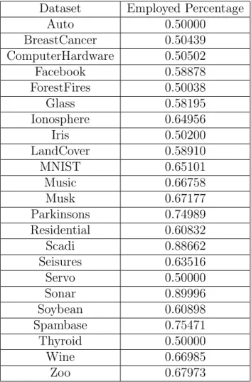
The artificial bee colony (ABC) algorithm is inspired by the intelligent behaviour of a honey bee swarm. In the ABC algorithm, the population is divided into three different parts: employed bees, onlooker bees, and scout bees [18]. Employed bees go to their food source and then return to the hive and dance on this area [18]. If an employed bees food source becomes abandoned, this bee will become a scout bee and search for a new food source. Onlooker bees watch the dances of employed bees and choose a food source based on the dance [18].

(12)

CHAPTER 1. INTRODUCTION 3

The bacterial foraging optimization (BFO) algorithm is inspired by the group foraging behaviour of E. coli and M.xanthus bacteria [27]. Specifically from these bacteria, the behaviour is inspired by the chemotaxis that perceives the chemical gradients in the environment and moves the bacteria towards or away from the source [27].

The bat algorithm is influenced by the echolocation techniques of microbats [46]. Each bat in the population flies randomly and modifies its echolocation impulses when it finds prey. The position of bats is updated in an iterative manner similar to PSO where a velocity and position update are influenced by previously found best solutions [46].

The firefly algorithm is inspired by the flashing behaviour of fireflies [45]. Based on this principle, fireflies are attracted to any other individual in the population. Fireflies move towards each other based on the brightness that they are currently exhibiting with the lower brightness firefly being attracted by the brighter one [45]. The brightness is related to the function that is being optimized.

The fish school search algorithm is inspired by the collective behaviour of a school of fish [6]. The school swims towards the better solutions in order to feed and gain weight. These feeding and weight gain operators influence the direction of the school which moves the fish into the areas where better solutions may be found [6].

In order to compare the abilities of these algorithms, 23 datasets were chosen from the UCI machine learning repository. There are 7 regression datasets and 16 classification datasets. The regression datasets are Forest Fires, Geographical Original of Music, Residential Building, Facebook Metrics, Auto, Computer Hardware, and Servo. The classification datasets are: Iris, Glass, Zoo, Wine, Parkinsons, Soybean, SCADI, Ionosphere, Musk V2, Breast Cancer, Connectionist, Thyroid, Seizures, Land Cover, Spambase, and MNIST.

(13)

generalize for both classification and regression problems. The algorithms will search for a set of connection weights by using 80% of the dataset as a training set. Once the training has completed, the remaining 20% of the dataset is used as the testing set.

The experiments in this thesis use every combination of algorithm, activation function, and dataset to compare how the other swarm-based algorithms perform relative to PSO. The measures that are collected for each algorithm include: training accuracy, training loss, testing accuracy, testing loss, saturation of hidden nodes, and a measure of overfitting.

It was found that particle swarm optimization was the best algorithm when exam-ining the traexam-ining accuracy and traexam-ining loss, but performance suffered when applied to the testing data. The overfitting indicator was used at this point to discover that particle swarm optimization was likely to overfit, which follows the results found when examining training versus testing results.

When using classification datasets, ant colony optimization, firefly algorithm, and fish school search all surpassed particle swarm optimization. Particle swarm opti-mization was the best performing algorithm for the regression datasets.

Ant colony optimization was found to be the algorithm that saturated the least, while also examining the relationship between the performance of Ant Colony Op-timization and how much or how little Ant Colony OpOp-timization saturated in those datasets. There is a relationship to be examined which follows the previous literature. This thesis is organized as follows: Chapter 2 includes an introduction to artificial neural networks. Chapter 2 also includes a detailed exaplanation of particle swarm optimization, ant colony optimization, artificial bee colony optimization, bacterial foraging optimization, bat algorithm, firefly algorithm, and fish school search. Lastly, Chapter 2 describes saturation and how this thesis will measure it, as well as over-fitting and how an overover-fitting indicator will be used in this thesis. Chapter 3 of this

(14)

CHAPTER 1. INTRODUCTION 5

thesis describes the literature in which swarm intelligence algorithms have been ap-plied previously to training artificial neural networks. Chapter 4 describes how each algorithm was implemented, Chapter 5 contains the parameters used for the artificial neural network architectures, as well as the parameters for each algorithm. Chapter 6 contains the rankings results for each of: loss, accuracy, saturation, and overfitting. Lastly Chapter 7 summarizes the results found and proposes some future work.

(15)

Chapter 2

Background Information

2.1

Swarm Intelligence Algorithms

Swarm intelligence (SI) algorithms use a system of agents that interact with their environment and other agents to guide the search to solve a problem []. This problem can be either a continuous or discrete optimization problem. These algorithms have the following properties:

• Composed of many individuals.

• Either identical individuals, or very few subclasses.

• Interactions between individuals follow simple rules that exploit only

informa-tion exchanged within the populainforma-tion or from interacting with the environment.

• This leads to the overall group behaviour of self-organization.

This thesis focuses on algorithms that are categorized as SI algorithms.

2.1.1

Particle Swarm Optimization

Particle swarm optimization (PSO) is a metaheuristic introduced by Kennedy and Eberhart [21]. The PSO algorithm was inspired by the flocking behaviour of birds.

(16)

CHAPTER 2. BACKGROUND INFORMATION 7

PSO maintains a population of solutions that are iteratively updated to move in the search space. Mathematical formulae are applied to every particle’s velocity and position. The velocity of a particle controls how fast the particle travels through the search space while the position of a particle represents the solution to the problem being explored. The calculations at each iteration are based on two positions that were previously found; the personal best location and the best position found in a neighbourhood. The particles are ranked based on the quality of the solution that they produce. In minimization problems, the best particle positions are the ones that produce the smallest fitness based on the function applied. The opposite is true for a maximization problem. The neighbourhood is a representation of how information is shared between particles; in a fully connected neighbourhood every particle has access to all of the information available, while other network topologies limit the amount of information available to each particle.

The velocity of a particle is calculated at each iteration using the following equa-tion:

vi(t+ 1) =ωvi(t) +c1r1(y(t)−xi(t)) +c2r2(ˆy(t)−xi(t)) (2.1)

where t is the current iteration, xi(t) is the current position of the particle at

dimension i, vi(t) is the current velocity of the particle at dimension i, yi(t) is the

personal best position of the current particle at dimension i, ˆyi(t) is the global best

position at dimensioni,ωis the inertial term, which applies a portion of the previous velocity to the next velocity,C1 is the cognitive component, which influences the effect of the personal best found position, C2 is the social component, which influences the effect of the global best found position, andR1 andR2 are random values in the range [0, 1]. The parameters ω, C1, and C2 have a major effect on the performance of the PSO algorithm. Typically the inertial term is in the range [0, 1], and the cognitive and social terms are in the range [0, 2]. The position of a particle is then updated

(17)

using the following formula:

xi(t+ 1) =xi(t) +vi(t+ 1) (2.2)

At every iteration, the updated velocity of a particle is added to the current position to generate the position of the particle in the subsequent iteration.

2.1.2

Ant Colony Optimization

The ant colony optimization (ACO) algorithm was introduced in [10] with aims to search for an optimal path in a graph. The ACO method is based on the ability of ants to search for a path between their colony and a food source. Initially, the ants will randomly choose paths to the food source. As the ants travel, they deposit pheromone along their path. This deposit leaves information for the next set of ants to travel to the food source using the same path.

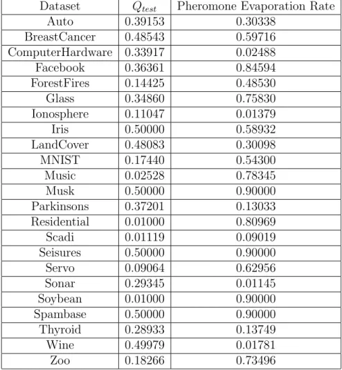
The ACO algorithm has been extended to optimize continuous valued problems, such as training an ANN. The initialization phase of ACO uses the number of inputs, outputs, and number of hidden nodes in the ANN to determine the length of the path to generate. Once the size of the path is found, each connection weight in the ANN is divided into d discrete points generated from a normal distribution. Additionally, each connection weight is also assigned an initial pheromone value using the formula:

τijh ←1/(ni+nh+no) (2.3)

where ni is the number of inputs, nh is the number of hidden nodes, and no is the

number of output nodes.

The ants in ACO each generate a solution to the problem to be optimized. At each iteration an ant probabilistically chooses a path to travel on based on pheromone information at that point. This probabilistic choice is generated through the following

(18)

CHAPTER 2. BACKGROUND INFORMATION 9 formula: ρijh = τijh Pd k=1τijk (2.4) whereρijh is the probability of selection path componentAijhforWij,drepresents the

number of discrete points, andτijh represents the existing pheromone trail associated

with Aijh. Once each ant has generated a complete solution the pheromone trails are

updated. Only the best ant updates the pheromone of the trails, using the formula:

τijh ←τijh+ ∆bestτ ijh,∀aijh ∈Tbest (2.5)

where Tbest _{is the best found combination of points, and ∆}best

τ ijh is the amount of

pheromone to be deposited which is defined as:

∆best_{τ ijh} = 1

Ebest (2.6)

whereEbest_{is the fitness of the solution generated by the best ant. Here, the better}

the quality of the solution, the lower Ebest_{, the more pheromone that is deposited.}

The pheromone is then updated using pheromone evaporation:

τijh ←(1−ρ)τijh,∀aijh (2.7)

where ρ is a constant in the range [0, 1]. This evaporation helps eliminate poor decisions made in previous iterations.

2.1.3

Artificial Bee Colony Optimization

The artificial bee colony (ABC) algorithm was introduced in [18]. The ABC algorithm is based on the collective behaviour of a bee colony in the search for food sources. ABC uses three different types of bees: employed bees, onlooker bees, and scout bees. The employed are located at a food source. These bees represent a solution to the

(19)

problem. A food source is generated using the formula:

xmi=li+rand(0,1)∗(ui−li) (2.8)

where li and ui are the lower and upper bounds for the position i, respectively.

The employed bees will search locally around their food source for other potential food sources. The number of employed bees is equal to the number of food sources found around the hive. Employed bees will determine a neighbouring food source using the following formula:

vmi=xmi+φmi(xmi−xki) (2.9)

where xk is a randomly selected food source, i is randomly chosen parameter index,

and φmi is a random number within the bounds (li, ui).

The onlooker bees will search around the hive for other food sources, based on the probability generated by the quality of the food sources that the employed bees are currently examining. Once a food source is probabilistically chosen, the onlooker bee then searches near that food source for a new food source. The probabilistic calculation is performed using the following formula:

pm =

f itm(x~m)

PSN

m=1f itm(~xm)

(2.10)

Once a food source is chosen, a new food source is created using Equation 2.9. If the fitness value of the new position is better than the current position, the current position is abandoned and the new position is used.

The last bee type is the scout bee. This type of bee attempts to find new food sources for employed bees once the previous food source has reached a set number of trials for searching by employed and scout bees. The new food source is created

(20)

CHAPTER 2. BACKGROUND INFORMATION 11

randomly using Equation 2.8. This balances the ABC algorithm’s exploitation and exploration of the search space.

2.1.4

Bacterial Foraging Optimization Algorithm

The bacterial foraging optimization algorithm (BFOA) was introduced in [27]. The BFOA algorithm is inspired by the social foraging behaviour of the E. coli and M. xanthus bacteria. This theory is inspired by the principle that animals search for and obtain nutrients in a fashion that maximizes the ratio ofE/T, whereE is the energy obtained and T is the time spent foraging.

The BFOA’s main goal is to minimize the function being used,J(θ) whereθ repre-sents the current position of a bacterium. J(θ) also represents a gradient information profile, where J < 0, J = 0, & J > 0 represent the presence of nutrients, a neutral position, and the presence of noxious substances, respectively [27]. Let:

P(j, k, l) = {θi(j, k, l)|i= 1,2, ..., S} (2.11)

represent the positions of each member in the population of the S bacteria at the

jth chemotactic step, kth reproduction step, andlth elimination-dispersal event. Let

J(i, j, k, l) denote the cost of the location of the ith bacterium. N c is the length of a bacterium lifetime, measured by the number of chemotactic steps [27]. To generate a tumble, a random unit length vector is generated then added to the current position of the bacterium. This is repeated until the cost at this next position is worse than the current position being examined, orN s, the number of chemotactic steps, is reached. The next step of the algorithm is to calculate the interactions between bacterium in the population. Let Dattract be the strength of the attractant released by the

current bacterium, and Wattract be the width of that attractant signal. Using local

(21)

height of the repellent effect and Wrepel as the measure of the width of the repellent, then using: Jcc(θ) = S X i=1 J_cci = S X i=1 "

−dattractexp(−wattract p X j=1 (θj −θij) 2₎ # (2.12) + S X i=1 "

hrepellantexp(−wrepellant p X j=1 (θj −θij)2 # (2.13)

where θ = [θ1, ...., θp]t is a point in the search space domain. The bacterium will

secrete attraction and repulsion chemicals affected by the environment, where a bac-terium with higher nutrient concentration will secrete stronger attractant than a bacterium with a low concentration.

After Nc chemotactic steps are taken, Nre reproduction steps are taken. In this

reproduction step, the healthiest half of the bacteria are kept while the rest are replaced with new bacteria. Lastly, the bacteria go throughNed Elimination Dispersal

steps, where bacteria are chosen randomly to elimination dispersal with probability

Ped.

2.1.5

Bat Algorithm

The bat algorithm (BA) is based on the echolocation capabilities of microbats, intro-duced by Yang in [46]. All microbats use echolocation to locate prey, obstacles, or other bats in their environment. For the BA some characteristics of different species of bats are generalized. These rules are:

1. All bats use echolocation to sense their distance, as well as the differences be-tween food, prey, and their background barriers.

2. Bats will fly randomly with velocity vi at position xi with a fixed frequency

(22)

CHAPTER 2. BACKGROUND INFORMATION 13

can automatically adjust the frequency of their echolocation pulses, as well as the emission rate of these pulses depending on the proximity of their target [46]. 3. Although loudness can vary in many ways, it is assumed that loudness varies

between a large positive value Ao to a minimum constant Amin.

It is assumed that there is no time delay or three dimensional topography concerns because of computational complexities in multiple dimensions.

In the BA bats are moved simply, generated by the following equations:

fi =fmin+ (fmax−fmin)β, (2.14)

v_it=v_it−1+ (xt_i−x∗)fi, (2.15)

xt_i =xt_i−1+v_it (2.16)

where β ∈ [0,1] is a random vector, x∗ is the global best position of all the bats.

Initial frequencies of bats are randomly chosen between [Fmin, Fmax]. A local search

is performed for each bat using a random walk:

xnew =xold+At (2.17)

where ∈[−1,1] is a random number and At _{is the average loudness of all the bats}

at this time step. The loudness Ai and rate of pulse emission Ri are updated each

iteration. As a bat finds prey the loudness decreases so any value can be chosen for the Amax [46]. The loudness and pulse emission rate is updated as:

At_i+1 =αAt_i (2.18)

(23)

where α and γ are constants and t is the current iteration. [46] defines that α and

γ can be the same. Bat positions, loudness, and pulse emission rate are randomly initialized [46]. The BA can be thought of as a balanced combination of the standard PSO algorithm with local search controlled by loudness and pulse rate [46].

2.1.6

Firefly Algorithm

The firefly Algorithm (FA), also introduced by Yang, is based on the flashing char-acteristics of fireflies [45]. Similar to BA, the following are assumptions that must be made about fireflies in the algorithm [45]:

1. All fireflies are unisex, so that one firefly will be attracted to all other fireflies regardless of their sex

2. Attractiveness is proportional to their brightness. Thus, for any two flashing fireflies, the less bright one will move towards the brighter one. If there is no brighter one than a particular firefly, it will move randomly

3. The brightness of a firefly is determined by the landscape of the objective func-tion

In the FA, two decisions must be made: the variation of light intensity, and the for-mulation of the attractiveness of fireflies. The attractiveness of fireflies is determined by the evaluation of the objective function for the position of that particular firefly. The light intensity varies according to the inverse square law:

I(r) =Is/r2 (2.20)

whereIs is the intensity at the source and ris the distance. For a given medium, the

light intensity varies with

(24)

CHAPTER 2. BACKGROUND INFORMATION 15

where I0 is the original light intensity. To avoid the singularity at r = 0 in equation 2.20, the combined effect of the inverse square law and absorption can be approxi-mated as:

I(r) = I0e−γr

2

(2.22) As this is proportional to a fireflies’ attractiveness, the attractiveness can be defined as:

β=βmine−γr

2

(2.23) where Betamin is the attractiveness at r = 0. The distance between any two fireflies

is the Cartesian Difference:

rij =||xi−xj||= v u u t d X k=1 (xi,k−xj,k)2 (2.24)

Lastly, the movement of a firefly i is attracted to another more attractive firefly is determined by:

xi =xi+β0e−γr

2 ij(x

j−xi) +αi (2.25)

where the second term is due to the attraction of two fireflies. The parameter gamma characterizes the variation of the attractiveness thus controlling the convergence and behaviour of the FA.

2.1.7

Fish School Search Algorithm

The fish school search (FSS) algorithm is inspired by the collective behaviour of fish schools [6]. The fish in the FSS population each have an innate memory of their successes through their weights. FSS also uses the concept of evolution through a combination of collective operators which are techniques that select different modes of movement. There are two operator groups; feeding and swimming [6]. The feeding operator uses food as a metaphor for indicating the regions of the search space that

(25)

are likely to be good areas for solutions. The swimming operator is a collection of operations that attempt to guide the global search process towards areas of the search space that are sensed by the population to be more promising.

Much like real fish, the FSS population of fish are attracted to food in the search space [6]. In order to find a greater amount of food, fish in the population are able to move independently. This allows each fish to grow or shrink in weight depending on the success or failure of finding food. The weight of the fish is then updated by the following formula:

Wi(t+ 1) =Wi(t) +

f[xi(t+ 1)]−f[xi(t))]

max{|f[xi(t+ 1)]−f[xi(t)]|}

(2.26)

where t is the current iteration, W i(t) is the current weight of the fish, Xi(t) is

the current position of the fish, and f[xi(t)] is the fitness function applied to the

current position. Other important information about the weight of the fish is that the weight is updated at each iteration, there is a maximum weight Wscale, and all

fish are initialized with weight equal to Wscale/2.

For FSS, fish swimming is directly related to all the important individual and collective behaviours such as feeding, breeding, escaping from predators, moving to more livable regions of the current habitat, or exploring socially [6]. This creates three types of movements for the FSS: individual, collective-instinct, and collective-volition. The first type of movement, individual, occurs for each fish at each iteration. This direction is randomly chosen and the fish then evaluates that position in the search space. If the position is within the bounds of the search and the food density at the new position is greater than the current position, the fish moves to this new position. This movement is also associated with a step size parameter,Stepind, which

determines the size of the movement. This parameter is decreased at each iteration. The next movement is the collective-instinctive movement. After the individual

(26)

CHAPTER 2. BACKGROUND INFORMATION 17

movement has completed, a weighted average of the individual movements of the population is calculated. The fish with success in moving individually influence the movement of the overall population more than unsuccessful fish. This movement is based on the following formula:

xi(t+ 1) =xi(t) + PN i=1∆xind i{f[xi(t+ 1)]−f[xi(t)]} PN i=1{f[xi(t+ 1)]−f[xi(t)]} (2.27)

where ∆xind i is the displacement of fish i due to the individual movement operator.

After computation, the positions of the population are then updated.

Last is the collective-volatile movement operator. This operator is based on the overall performance of the population. It follows the following logic: if the population is putting on weight, indicating the search is successful, then the radius of the popula-tion will contract. Otherwise the radius will dilate. The collective-volatile movement operator is deemed to help greatly in enhancing the exploration abilities of the FSS. This operator is applied to each position of each fish in the population in regards to the population barycenter. The barycenter is calculated by the following formula:

Bari(t) = PN i=1xi(t)Wi(t) PN i=1Wi(t) (2.28)

This movement operator will be inwards or outwards compared to the population barycenter. Fish position is then updated with the following formula.

xi(t+ 1) =xi(t)−stepvolrand(0,1) [xi(t)−Bari(t)] (2.29)

xi(t+ 1) =xi(t) +stepvolrand(0,1) [xi(t)−Bari(t)] (2.30)

If the weight of the population has increased then use 2.29, otherwise use 2.30. The

Stepvol parameter is also decreased like the Stepind parameter at each iteration using

(27)

step(t) = stepinitial−sqrt[(1−t2/a2)∗b2] (2.31)

where ais the maximum number of iterations, b is the distance between Stepindinitial

and Stepindf inal, andt is the current iteration.

2.2

Artificial Neural Network

The artificial neural network (ANN) is a model that simulates the structure and behaviour of biological neurons. These artificial neurons are interconnected and have weights that are associated with these connections. The artificial neurons and weights are the building blocks of an ANN. ANNs are trained by weights that connect neurons. Weight updating is performed by using feedback from the error rate of the network output compared to the target output. When training is performed correctly, an ANN can be used to produce correct outputs for new unseen data.

Figure 2.1: A Simple Neuron

The most basic ANN component is the artificial neuron, seen in Figure 2.1. The artificial neuron has 3 basic components: weights, a summation, and an activation function. The weights are multiplied by the input to the node. The weights represent the inherent relationship between the input data and its importance in determining

(28)

CHAPTER 2. BACKGROUND INFORMATION 19

the output of the network. If the weight is positive, then data is passed further into the network. Alternatively, if the weight is negative, data is inhibited from being passed further into the network. Next, the summation sums the results of the mul-tiplication of the inputs and the weights. This singular value is then passed through the activation function. This function must be nonlinear to allow for nonlinear re-lationships to be modelled. The activation function is further explained in Section 2.3.

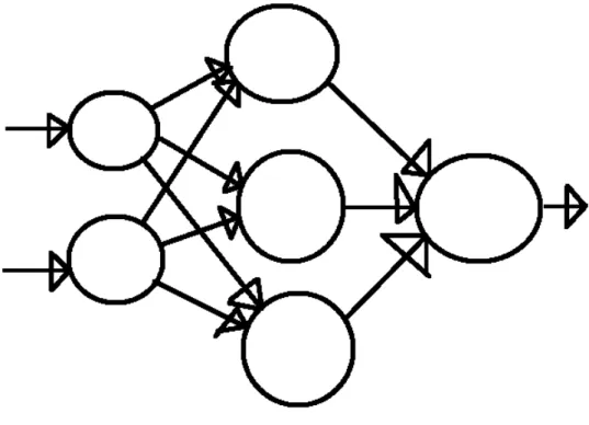
A multi-layer ANN consists of three types of layers. The first is an input layer; this layer accepts the data as input and takes on the values of the data. There is no weight associated with the input to the input layer. Next is one or more hidden layer(s). The number of layers used is determined by the problem that needs to be solved. In this thesis, ANNs with only one hidden layer are used. The hidden layer takes the values from the input layer and follows the procedure of multiplying the connection weights by the input, summing the result, and passing the result through the activation function.

The last layer in an ANN is the output layer, which produces values that are related to the target class of the problem being passed to the ANN. This layer performs the same multiplication, summation, and application of the activation function as the hidden layer and outputs this value which is related to the task at hand. If the problem associated with this task is a classification task with two or more classes, the ANN output layer may contain a single output node that outputs values and these values must be interpreted as classes. Otherwise, the output layer could contain the same number of nodes as there are target classes (ie 10 target classes, 10 nodes in the output layer). In this case, the network would output a probability for each node in the layer that indicates how certain the model is about which class the input data is associated with. Alternatively, if this is a regression-type problem, the output layer consists of one output node that will produce a value that is related to the problem

(29)

Figure 2.2: An Artificial Neural Network

being examined. For example, the network could output a predicted grade of 74.5721 for a prediction of how a student will do on a future test.

2.3

Activation Functions

The activation function of a ANN is the component that allows for a non-linear relationship to be modelled by the ANN. Some examples of activation functions can be seen in the following subsections.

2.3.1

Sigmoid Function

The sigmoid activation is defined as

(30)

CHAPTER 2. BACKGROUND INFORMATION 21

and has an output range of (0, 1).

Figure 2.3: The Sigmoid function.

2.3.2

Hyperbolic Tangent Function

The Hyperbolic Tangent function, referred to as Tanh, is defined as

f(net) = (enet−e−net)/(enet+e−net) (2.33)

and has an output range of (-1, 1)

(31)

2.3.3

Lecun’s Hyperbolic Tangent

Lecun’s Hyperbolic Tangent function, referred to as Lecun’s Tanh, was suggested in [25] and is defined as

f(net) = 1.7159etanh(2

3net) (2.34)

When compared to the Sigmoid function, Lecun’s Tanh has a softer slope and wider output range of (-1.7159, 1.7159).

Figure 2.5: The Lecun Hyperbolic Tangent function.

2.3.4

Elliot

The Elliot activation function, hereby referred to as Elliot, is suggested in [34] and is defined as

f(net) =net/(1 +net) (2.35) This function has an output range of (-1, 1) but has a shallower gradient than Tanh, thus approaching the asymptotes slower.

(32)

CHAPTER 2. BACKGROUND INFORMATION 23

Figure 2.6: The Elliot function.

2.4

Saturation

When using bounded activation functions, it can be measured how much the hidden units in an ANN have saturated. Provided that there are enough neurons in the hidden layer, a nonlinear activation function allows the ANN to approximate any nonlinear relationship [23]. The bounds on the activation functions ensure that the signal does not grow wildly as signals propagate from layer to layer. When the input to a sigmoidal function is between the bounds of the function, the output exhibits linear behaviour. When the input to that same Sigmoidal function is outside of the bounds of the function, the output of the Sigmoidal function approaches the asymptotes, referred to as saturation. This effectively renders an ANN into a binary output state where the output of any input, with only one value outside of the activation bounds of the function, will be pushed to the asymptotic bounds of the function depending on the sign of the input.

This phenomenon is unsatisfactory in the training of an ANN since a small change in the input to a neuron will have no effect on the output of that neuron. Thus, any algorithm that attempts to change the weights of an ANN will find it difficult to evaluate whether changes to weights affects the output of the ANN, causing learning

(33)

to stall.

To further illustrate this problem, a Sigmoidal function is used in the output layer and a binary classification problem is considered. Given this, it may seem correct that saturated outputs should be found. However, in [23] it was found that a saturated output does not indicate how confident the ANN was in outputting that class. Instead, the ANN outputs the same confidence level for each example in the training set, preventing the ANN from improving on the current solution.

2.4.1

Measure of Hidden Unit Saturation

This thesis will use the measure found in [38] to measure the rate at which each algo-rithm saturates in the hidden layer. First, a frequency distribution is generated from the outputs of the hidden layer. This frequency distribution can then approximate the level of saturation generated by this ANN training algorithm. Next, a single val-ued saturation measure can be derived from the frequency distribution. The average output signal for each bin b can be calculated from the hidden layer outputg(net) as follows: ¯ gb =      (Pfbg(net)k k=1 )/fb if fb >0 0 otherwise      (2.36)

wherefb is the number of output signals in binb. If the range of ¯gb is centered around

0, the absolute average will be higher for bins closer to the asymptotic values and lower for bins closer to the centre. If the range of g is [gL, gU],gbcan be scaled to -1,

1 as follows: ¯ gb0 = 2( ¯gb −gL) gU−gL −1 (2.37)

A weighted mean magnitude is then calculated as :

ϕB= B X b=1 |g¯b0|fb B X b=1 fb (2.38)

(34)

CHAPTER 2. BACKGROUND INFORMATION 25

where B is the total number of bins, and fb constitutes the weight of each bin. The

weighted mean is the same as the arithmetic mean if the weights are equal. If the frequency was distributed uniformly in [-1, 1] then the value of ϕB will be 0.5. For a normal distribution in the frequency distribution the value of ϕB will be less than 0.5, the higher the asymptotic frequencies the closer the value ofϕB is to 1. In other words, asϕB trends towards 1 the more saturation in the ANN. It was found in [38] that a value of 10 for the number of bins, b, is acceptable for measuring saturation.

2.5

Overfitting

The goal of ANN training is to learn the important features of the data so that the ANN can accurately classify unseen data. Typically, this is done by partitioning the dataset into three exclusive sets: training, validation, and testing. The ANN uses the training set as the data that is passed through the network to generate an output to use for Backpropagation. The validation set is used as a performance measure after every epoch of training. This set is used as an indicator of future success on previously unseen data. Lastly, the testing set is used as actual indication of success on unseen data. This set of data does not include any training example that the ANN has seen before.

Overfitting of an ANN occurs when the ANN learns to approximate the nonlinear relationship of the training data too closely. This can be described as the ANN has memorized rather than generalized, where it seems like the ANN memorized the target classes of the training set and did not generalize for the testing set. Overfitting can occur due to factors such as limited training data, too many free parameters to optimize, or too many training epochs.

(35)

2.5.1

Indication of Overfitting

Overfitting in ANN training is the phenomenon in which the ANN has adequate performance on the training dataset but poor performance on the testing dataset or any other unseen data. This can be the result of having too many free parameters which then learns the noise of the dataset. A generalization factor was developed in [39] which is an indication of overfitting behaviour of an ANN. The indicator is

pf = etest

etrain

(2.39)

where etest is the loss on the testing dataset, and etrain is the loss on the training

dataset. It is desirable to have a pf < 1 which indicates that generalization error is less than the training error. A pf > 1 indicates that the generalization error is greater than the training error which may indicate overfitting. In this thesis pf is used to describe the overfitting behaviour of an algorithm and not as a measure of overfitting where this indicator may be able to aid in explaining behaviours of the SI trained ANNs instead of being a way to compare how overfit a network is.

(36)

Chapter 3

Swarm Intelligence Algorithms

Previous Work

This is a section that describes swarm intelligence algorithm application to ANN training.

3.1

Particle Swarm Optimization

Particle swarm optimization (PSO) has been applied to the ANN training in multiple domains, including the evaluation of nonlinear functions, medical diagnoses, engi-neering, computer vision, and geography. In [14] it was found that PSO requires less iterations of training to achieve a similar level of error as the backpropagation algo-rithm. [32] applied PSO to train ANN for medical diagnoses where there was a small sample size a large number of features, and correlations between the available features. [32] found that backpropagation is generally preferred over PSO for imbalanced train-ing data with a small number of samples and a large number of features. [47] applied PSO to adapting the ANN architecture as well as the connection weights, applying this technique to two real problems in the medical domain, finding that this technique provided good accuracy as well as good generalization ability. [33] applied PSO to a selection of classification and regression problems, such as N bit Parity, Three Color

(37)

Tube, Diabetes in Pima Indians, Sin Times Sin, and Rise Time Servomechanism. PSO was shown to be more robust when there is a high number of local minima [33]. [8] applied PSO to training ANNs while also applying PSO variants, backpropagation variants, and Hybrid approaches between PSO and backpropagation using backprop-agation variants as a local search mechanism. It was shown that PSO was successful when applied to the Diabetes dataset [8]. A comparison was performed in [22] where multiple ANN training approaches were applied to four classification datasets as well as an e-Learning dataset. These approaches included PSO, Genetic Algorithm, bat algorithm, and Levenberg-Marquardt algorithm. It was found in [22] that the bat algorithm was more useful when applied to these datasets. [43] investigates the over-fitting behaviour of PSO trained ANNs. [43] found that the PSO topology influenced the overfitting behaviour, as well as the use of bounded activation functions. [43] also witnessed non-convergent behaviour in the PSO swarm which was attributed to the use of bounded activation functions. When unbounded activation functions were used, it was found that the PSO swarm converged while overfitting behaviour was drastically reduced [43].

While the previously mentioned literature discusses PSO’s ability to train an ANN, none of the literature attempts to discuss why this may be. [37] hypothesized that the deficiency of PSO may be due to hidden layer saturation. [37] found that while a certain degree of saturation was required for ANN success, higher levels of satura-tion was found to be unsatisfactory and would lead to overfitting. [43] found that non-gradient based learning can be sensitive to the degree of saturation present in an ANN. [38] devised a method to measure the degree to which an ANN has saturated that trends towards one for a more saturated ANN and zero otherwise. [38] applied four activation functions to their datasets, Sigmoid, Hyperbolic Tangent, Elliot, and Lecun’s Hyperbolic Tangent, finding that Lecun’s Hyperbolic Tangent function sat-urates the least. Through the review of the literature that has been presented here,

(38)

CHAPTER 3. SWARM INTELLIGENCE ALGORITHMS PREVIOUS WORK 29

it can be noted that PSO suffers in training ANNs when compared with more tradi-tional ANN learning techniques. This may be because of PSO not performing well in high dimensions, hidden unit saturation, or the overfitting behaviour.

3.2

Artificial Bee Colony Optimization

The artificial bee colony (ABC) algorithm has been applied to the training of ANNs in previous works with mild levels of success. [19] used the ABC algorithm to train ANNs for 3 benchmark functions: XOR, 3-bit parity, and 4-bit Encoder-Decoder. [19] found that the ABC algorithm produced accurate ANNs when applied to these three benchmark functions. In [20] it was found that ABC trained ANNs outper-formed backpropagation trained ANNs. [40] applied ABC trained ANNs to predict overall heart function from electrocardiogram signals. [40] found that this ANN per-formed very satisfactorily while also reducing the time taken to train this ANN. [3] applied the ABC algorithm to train ANNs for Crime Classification. [3] found that the ABC-trained ANNs outperformed other Machine Learning algorithms, includ-ing backpropagation trained ANNs, Decision Trees, and Naive Bayes classifier. [36] used the ABC algorithm to train ANNs for modeling the daily evapotranspiration equation. [36] found that the ANNs generated were superior to the ANNs generated using the backpropagation ANNs. [41] applied the ABC-trained ANNs to predict the temperature of a volcano based on time-series data. [41] found that the basic ABC algorithm outperformed the backpropagation-trained ANNs. Lastly, [5] found that when the ABC algorithm is applied to short-term electric load forecasting for power generation planning, transmission dispatching, and day-to-day utility operations, that the ABC algorithm produces ANNs that are more suitable for this problem than PSO or Genetic Algorithms.

(39)

3.3

Ant Colony Optimization

The ant colony optimization (ACO) algorithm is, in its original state, an algorithm that is used for discrete optimization problems such as the Travelling Salesperson problem. Thus, some design decisions must be made to convert this algorithm into a discrete optimization algorithm. This conversion was first performed in [28]. At every decision point, the ant must choose a discrete point that represents a connection weight at that specific location. Once a solution was fully constructed, [28] applied backpropagation to perform a local search. [30] then applied this framework while also modifying the pheromone trail limit to allow for more search to occur as the number of iterations increases. [30] did also use backpropagation for local search once a solution was constructed. Lastly [31] built on the previous work in [30]. [31] applied ACO to nine benchmark datasets and found that ACO was superior at training ANNs for three datasets when compared to Levenberg-Marquardt, backpropagation, and ACO with backpropagation.

3.4

Bacterial Foraging Algorithm

The bacterial foraging optimization (BFO) algorithm has been used in specific ap-plications. The first example of this is in [13] where BFO was used to create ANNs that are used to protect large power transformers. The BFO-trained ANN were then found to be a robust solution to this problem. [44] then used BFO to train ANNs to predict Alzheimer’s disease, while attempting to identify the structural characteristics at baseline and over a period of two years. [44] reported an accuracy of about 92% using this approach which indicates that this is an acceptable approach.

(40)

CHAPTER 3. SWARM INTELLIGENCE ALGORITHMS PREVIOUS WORK 31

3.5

Bat Algorithm

Initially the bat algorithm (BA) was applied in [35] in combination with backprop-agation to determine the efficiency of BA when applied to training ANNs. When compared to ABC with backpropagation or backpropagation alone, [35] found that BA with backpropagation was superior. [42] applied BA to a selection of benchmark datasets where it was found that BA performed similarly to other metaheuristics, while a modified BA outperformed every other algorithm that was tested. Next [2] applied the BA to image compression where the relationship between each pixel can be nonlinear. The BA was also applied in [26] to help improve machining accuracy in thermal error modeling. [26] found that the BA with backpropagation is more stable and has higher prediction accuracy, providing a solid candidate for thermal error modeling.

3.6

Firefly Algorithm

Lastly, the firefly algorithm (FA) was applied in [17] to train an ANN to recognize characters gathered from Microsoft Paint. [17] found that the proposed FA with back-propagation technique performed better and converged quicker than other methods. Next [7] used FA to train an ANN for classification problems, namely XOR, 3-bit par-ity, and 4-bit Encoder-Decoder. [7] found that the ABC algorithm performed better comparatively, but FA outperformed a Genetic Algorithm. Next FA was used in [29] with backpropagation on a randomly generated dataset. [29] found that the FA did not perform well because of a lack of data, a small population of fireflies, and a low number of iterations. Lastly [15] used FA in conjunction with backpropagation for solving hydrogeneration predictions. [15] found that this approach resulted in better ANNs in terms of speed of ANN training and accuracy of predictions.

(41)

3.7

Problem Definition

As noted in Section 3.1, PSO suffers from hidden unit saturation and has some over-fitting behaviour. While other SI algorithms have been applied to ANN training, no work has been done to compare the effectiveness of these other algorithms with performance, hidden unit saturation, and overfitting behaviour in mind. This thesis aims to compare the performance of SI algorithms with these metrics in mind.

(42)

Chapter 4

Implementation

This is a section that examines the implementation details of each algorithm. Each al-gorithm in this thesis was implemented using the Python 3.6.3 programming language [1]. Each algorithm used a population size of 50 for 1000 iterations, except for the BFO algorithm which uses a variable number of iterations depending on the problem. The fitness function of each algorithm was a forward pass of an ANN. This forward pass involved taking the position of the current solution as a parameter, splitting the solution into weights and biases, and then performing the resulting multiplications to generate a result for that solution.

The fitness of each algorithm was set to be a forward pass of data through an ANN by converting a solution’s position into an ANN. If the dataset was classification based, then the fitness was the Cross-Entropy loss. If the dataset was regression based, the fitness was the Mean-Squared Error loss.

4.1

Particle Swarm Optimization

For the PSO implementation, a fully connected topology was used that shared global best information among each of the members of the population. The velocity of each particle was restricted to the range [−1,1] as performed in [38] to reduce the divergence of the PSO swarm and the synchronous version of PSO was used. The

(43)

basic algorithm can be seen in Algorithm 1.

Algorithm 1 Particle Swarm Optimization Algorithm

while Generation <1000 do for Particles in Population do

Evaluate Fitness Update Personal Best

end for

Update Global best

for Particles in Population do

Update Velocity

Update Particle Position

end for end while

4.2

Artificial Bee Colony

The implementation of the ABC algorithm is based on [18]. This implementation represented food sources as solutions, encapsulating the number of trials, current position, and current fitness inside of this food source. This algorithm can be found in Algorithm 2.

Algorithm 2 Artificial Bee Colony Algorithm

while Generation <1000 do

Each Employed bee goes to it’s food source and searches locally using Equation 2.9

if Fitness(Current Food Source)> Fitness(New Food Source)then

Keep the new found food source

end if

Each Onlooker Bee then probabilistically chooses a food source to search around for better food source(s) using Equation 2.10

if Fitness(Current Food Source)> Fitness(New Food Source)then

Keep the new found food source

end if

Scout Bees will search for new food sources once a previous food source is depleted using Equation 2.8

(44)

CHAPTER 4. IMPLEMENTATION 35

4.3

Ant Colony Optimization

Next the ACO algorithm was implemented. This implementation is based on [31] where 30 discrete points are used for each connection weight, the pheromone trails evaporate at a certain rate. The basic flow of ACO can be seen in Algorithm 3.

Algorithm 3 Ant Colony Optimization

Initialize Pheromone table using Equation 2.3

Probabilistic Solution Construction where an Ant chooses a value for each node in the ANN using Equation 2.4

Evaluate Fitness of the Generated ANN Find the Best Solution

Update Pheromone values using Best Solution using Equations 2.5 & 2.6 Apply Pheromone Evaporation using 2.7

end while

4.4

Bat Algorithm

The BA implementation is directly related to the pseudocode from [46] as well as a Matlab implementation that can be found in [45]. This algorithm can be found in Algorithm 4.

4.5

Bacterial Foraging Optimization

The BFOA implementation is based on the description from the original paper [27]. This algorithm can be found in Algorithm 5.

4.6

Fish School Search

The FSS algorithm was implemented based on [6]. [16] proposed that both the In-dividual and Volatile step sizes decrease non-linearly to allow for the areas around

(45)

Algorithm 4 Bat Algorithm

Initialize Population, Velocity, Frequency, Pulse Rate, and Loudness

Move bats using Equations 2.14, 2.15, & 2.16 generating new solutions Evaluate Fitness of Bats

for Bats in Population do

if rand()> Pulse Rate of Bat then

Generate a solution around the selected bat

end if end for

for Bats in Population do

Generate a new Solution by Flying randomly using Equation 2.17 around cur-rent bat

if random() < Loudness of Current Bat & Fitness(Current) > Fitness(New Solution) then

Accept the new solution

Decrease Loudness using Equation 2.18 & Increase Pulse Rate using Equa-tion 2.19

end if end for

Find current Best Bat

end while

the global minimum to be searched in more detail while also potentially speeding up the convergence to the global minimum. The formula for this decrease is found in Equation 2.31. This algorithm can be found in Algorithm 6.

4.7

Firefly Algorithm

The Firefly algorithm was implemented based on the Matlab code provided by Xin She Yang in [45].This algorithm can be found in Algorithm 7.

(46)

CHAPTER 4. IMPLEMENTATION 37

Algorithm 5 Bacterial Foraging Optimization Algorithm

for l = 0 toNed do

for k = 0 to Nre do

for j = 0 to Nc do

Apply a random vector to the current position

Calculated cell to cell interactions using Equations 2.12 & 2.13

if Fitness(Current) <Fitness(Current + Random) then

Break

end if end for

Update best cell found

end for

Sort Population by Fitness

Eliminate worst half of population

for Cells in population do if rand < Ped then

Create new cell at random location

end if end for end for

Algorithm 6 Fish School Search

while Generations< 1000 do for Each Fish in Population do

Move Fish individually by applying a random vector Evaluate Fitness

Update weight of fish with Equation 2.26

end for

Apply Collective-Instinctive Operator which is a weighted average of individual movements

Shrink or Expand the radius of the Population using Equations 2.28, 2.29, & 2.30 based on Individual Fish Success

Decrease Stepind & Stepvol using Equation 2.31

(47)

Algorithm 7 Firefly Algorithm

while Generation< 1000 do

for i= 1 : N umberOf F iref liesdo for j = 1 : ido

if Ij > Ii then

Vary attractiveness with distance r via exp(−γR) Move firefly i towardsj

Evaluate new solution and update light intensity I

end if end for end for end while

(48)

Chapter 5

Experimental Setup

This is a section that describes the experiments to be conducted.

5.1

Neural Network Architectures

In this thesis, only ANNs with 3 layers are used; one input layer, one hidden layer, and one output layer. The input layer is how data is passed through to the network, where the number of input nodes is equal to the number of attributes of the dataset. The output layer of the ANN depends on the type of dataset being used, and the number of output classes in the dataset. The number of nodes in the output layer for a classification problem is equal to the number of classes present in the dataset. The number of nodes in the output layer for a regression problem is equal to the number of target outputs in the dataset. The hidden layer contains any number of hidden nodes. At the time of writing, there is not a singular best way to obtain this number of hidden nodes. In this thesis, the number of hidden neurons for some datasets were taken from literature, as indicated by the citation in Table 5.1. If the number of hidden neurons could not be found in any literature, a Genetic Algorithm was used.

(49)

Dataset Number of Neurons Iris [11] 4 [38] Soybean [11] 6 [31] Facebook [11] 100 Seizures [11] 30 Forest Fires [11] 100 Musk V2 [11] 70 Auto [11] 50 Computer Hardware [11] 40 Glass [11] 9 [38] Spambase [11] 30 Servo [11] 50 Residential [11] 100 Parkinsons [11] 20 Music [11] 40 Breast Cancer [11] 6 [31] Sonar (Connectionist) [11] 30 Thyroid [11] 6 [31] Scadi [11] 20 Wine [11] 10 [43] Ionosphere [11] 5 Zoo [11] 10 Land Cover [11] 200 MNIST [24] 100

(50)

CHAPTER 5. EXPERIMENTAL SETUP 41

5.1.1

Defining Number of Hidden Neurons

The method of optimizing the Number of Hidden Neurons in this thesis is to use a Genetic Algorithm. The Genetic Algorithm used in this thesis was implemented using the Keras ANN framework. Keras is a machine learning framework designed for easy prototyping of ANN models written in Python. The Genetic Algorithm would gen-erate potential ANNs, train and test the ANN, and then new ANNs would be tested through the Genetic Algorithm operators of Crossover, Selection, and Mutation. So-lutions in a Genetic Algorithm are represented by chromosomes. Each chromosome is a an object with information about the ANN: the number of hidden nodes, the learning rate, and the activation function. The number of hidden nodes were set in increments of five, ranging from five to a maximum of 500. The fitness of these chromosomes was set to be the loss of the network that the chromosome generates. In classification tasks, Cross Entropy loss was used while Mean Squared Error was used in regression tasks.

With this Chromosome representation, crossover between chromosomes was a ran-dom choice between the two selected parents for each value available. Tournament Selection with k = 4 was used. In this Selection mechanism, four potential parents are chosen from the current population. These parents are then compared to find the one with the lowest fitness. The chromosome with the lowest fitness is then added to the pool of potential parents. Random pairs of chromosomes are chosen from this pool of parents to mate and generate the next two new chromosomes which become the next generation of chromosomes.

With the Genetic Algorithm approach, the number of hidden neurons for each dataset was tested to find an acceptable number of hidden neurons based on the performance of the network when trained using Backpropagation. This structure was then used in for every test with that dataset. The number of hidden neurons used for each dataset can be seen in the following table.

(51)

5.2

Parameter Tuning for each experiment

Bayesian Optimization (BO) was used to tune the parameters for each experiment. BO is a method of optimizing an objective function that are computationally expen-sive to evaluate [12]. BO consists of two components, a Bayesian statistical model for modeling the objective function and an acquisition function for deciding which parameters to test with next [12]. The statistical model is a Gaussian process which provides a Bayesian posterior probability distribution that describes potential values for some function f(x) at point x [12]. After each evaluation of f(x), the posterior dis-tribution is updated so good values of x can be found [12]. In this thesis, the function f(x) is a swarm intelligence algorithm and x is the parameters of the current algo-rithm. For each combination of SI algorithm, activation function, and dataset, BO is used to tune the parameters of the algorithm. The swarm intelligence algorithms in this thesis were implemented in Python so the BO was performed using GPyOpt. GPyOpt is an open-source library for BO developed by the Machine Learning group of the University of Sheffield [4]. This package boasts capabilities of automatic config-uration of models and Machine Learning algorithms, parallel experiments, and mixed types of variables [4].

5.3

Experimental Parameters

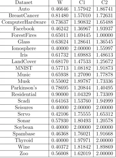
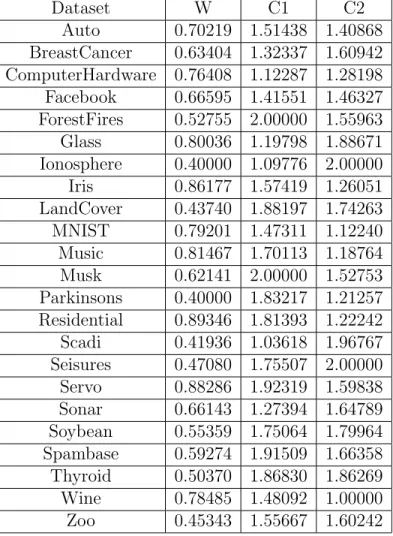
The GPyOpt package was applied to tune the parameters for each combination of algorithm, activation function, and dataset. The parameters were tuned in the fol-lowing ranges. The folfol-lowing tables contain the parameters that were used for each algorithm, activation function, dataset combination. An example of these parameters are found in Table 5.2 with the remaining parameters found in Section A.

(52)

CHAPTER 5. EXPERIMENTAL SETUP 43 Dataset W C1 C2 Auto 0.42434 1.82755 1.58621 BreastCancer 0.60270 1.89159 1.13346 ComputerHardware 0.77202 1.37043 1.51437 Facebook 0.79332 1.72871 1.46039 Forest Fires 0.56748 1.77542 1.09125 Glass 0.63589 1.37756 1.00825 Ionosphere 0.90000 1.00000 1.00000 Iris 0.49452 1.57499 1.98687 LandCover 0.68048 1.22115 1.17707 MNIST 0.40000 1.74774 1.91942 Music 0.70335 1.46544 1.97039 Musk 0.57469 1.73502 1.69297 Parkinsons 0.44225 1.42556 1.51641 Residential 0.90000 2.00000 2.00000 Scadi 0.40000 1.51375 1.00000 Seisures 0.40000 1.92354 1.92764 Servo 0.55772 1.30412 1.68724 Sonar 0.69614 1.54019 1.92433 Soybean 0.71224 1.51943 1.50465 Spambase 0.40000 1.80524 2.00000 Thyroid 0.52957 2.00000 1.90449 Wine 0.90000 1.00000 2.00000 Zoo 0.69983 1.54484 1.87629

(53)

Chapter 6

Results

This section describes the results found after performing the experiments. The first section describes results based on only the regression datasets, the second section only the classification datasets, the third section focuses on overall results, the fourth section examines the hidden unit saturation of each algorithm and activation function combination, while the last section describes the overfitting behaviours of each of the algorithms. Both the regression and classification sections will examine the results from two perspectives; training and testing, while the classification section will also include accuracy and loss results. The regression section will only focus on the loss results. Rankings for all algorithms were performed using the Wilcoxon rank sum test as described in [9]. Using this method, all algorithms can be given a rank based on how they perform on average across all activation functions on a given dataset. This ranking can then be averaged to generate an overall average rank which is used to rank the algorithm for an overall rank.

Lastly the results will be examined through the size of the dataset that was being used. The datasets will be split into small, medium, and large. Small datasets will have less than 500 instances or less than 50 features. Medium datasets will have more than 500 instances or more than 50 features. Large datasets will have more than 10,000 instances or more than 500 features. The small datasets are: Auto, Glass,

(54)

CHAPTER 6. RESULTS 45

Iris, Parkinson’s, Wine, Zoo, Computer Hardware, Ionosphere, Servo, and Soybean. Medium datasets are: Thyroid, Breast Cancer, Facebook, Forest Fires, Land Cover, Music, Musk, Sonar, Residential, Scadi, Seizures, Spambase. Lastly, the large dataset is MNIST.

6.1

Regression Results

First, the testing loss of the regression datasets must be examined. These results, shown in Table 6.1, are similar to the training loss results. Much like the training loss, PSO generated the best networks for testing loss based on the rank and the number of times that PSO generated the network that was ranked first for a dataset. Again, the BA followed PSO in second, with BFA & ACO moving up to third. Next it was observed that FSS remained in fifth, ABC moved down a rank to sixth, with Firefly remaining in seventh. It would be worthwhile to note that PSO did not generate all of the first ranked ANNs when examining the First Rank frequency. When examining the testing loss rankings it can be seen that BA produced two of the top performing networks, while BFA and FSS both produced one. This could be due to either hidden unit saturation or overfitting but will be examined in more depth in Section’s 6.4 & 6.5. For now, it can be said that when using an SI algorithm for a regression problem that PSO would be the most robust algorithm to use based on the performance shown in this section.

6.2

Classification Results

Next the performance of the SI algorithms in regards to loss will be examined. The firefly algorithm was found to be the top performer in this set of rankings, producing six of the top generated ANNs. Following Firefly was ACO, with one top ANN gener-ated, FSS in third while producing five top ANNs, PSO in fourth with four top ANNs,

(55)

Algorithm PSO ABC ACO BA BFA Firefly Fish Auto 1 4 2 3 5 7 6 ComputerHardware 1 6 7 1 1 1 5 Facebook 2 5 4 1 3 7 5 ForestFires 1 5 2 3 6 7 4 Music 1 6 4 2 3 7 4 Residential 1 7 4 3 2 6 5 Servo 1 5 3 2 6 7 4 Average Rank 1.1429 5.4286 3.7143 2.1429 3.7143 6 4.714 Ranking 1 6 3 2 3 7 5 First Frequency 6 0 0 2 1 1 0

Table 6.1: Testing Loss Regression Datasets

ABC in fifth, BA in sixth, and BFA in seventh; each with one top ANN generated. This is the first time in this thesis that PSO was not the top ranked algorithm. This ranking indicates that there may be better algorithms to use for training ANNs for classification than PSO. This will be further examined when examining the accuracy generated by these same networks.

Lastly the accuracy of the ANNs must be examined. These results can be found in Table 6.3. For the second time in the classification r