A genetic solution based on lexicographical goal
programming for a multiobjective job shop
with uncertainty
ARTICLE in JOURNAL OF INTELLIGENT MANUFACTURING · JANUARY 2010
Impact Factor: 1.14 · DOI: 10.1007/s10845-008-0161-x
CITATIONS
12
DOWNLOADS48
VIEWS124
3 AUTHORS:Ines Gonzalez Rodriguez
Universidad de Cantabria
41PUBLICATIONS 146CITATIONS SEE PROFILE
Camino Rodríguez Vela
University of Oviedo
62PUBLICATIONS 287CITATIONS SEE PROFILE
Jorge Puente Peinador
University of Oviedo
50PUBLICATIONS 193CITATIONS SEE PROFILE
Available from: Ines Gonzalez Rodriguez Retrieved on: 10 July 2015
Noname manuscript No.
(will be inserted by the editor)
A Genetic Solution based on Lexicographical Goal
Programming for a Multiobjective Job Shop with
Uncertainty
In´es Gonz´alez-Rodr´ıguez · Camino R. Vela · Jorge Puente
Abstract In this work we consider a multiobjective job shop problem with uncertain durations and crisp due dates. Ill-known durations are modelled as fuzzy numbers. We take a fuzzy goal programming approach to propose a generic multiobjective model based on lex-icographical minimisation of expected values. To solve the resulting problem, we propose a genetic algorithm searching in the space of possibly active schedules. Ex-perimental results are presented for several problem in-stances, solved by the GA according to the proposed model, considering three objectives: makespan, tardi-ness and idletardi-ness. The results illustrate the potential of the proposed multiobjective model and genetic algo-rithm.
Keywords Job shop scheduling, Uncertain duration, Multiobjective optimisation
1 Introduction
Scheduling problems form an important body of re-search since the late fifties, with multiple applications in industry, finance and science (Brucker and Knust, 2006). Part of this research is devoted to fuzzy schedul-ing, in an attempt to model the uncertainty and vague-Corresponding author. Dep. Mathematics, Statistics and Computing, University of Cantabria. Los Castros s/n, San-tander, 39005, Spain. E-mail: [email protected]; Tel: +34 942202201; Fax: +34 942 201402
A.I. Centre and Dep. of Computer Science, University of Oviedo. Campus de Viesques s/n, Gij´on, 33271, Spain. E-mail: [email protected]; Tel: +34 985182134
A.I. Centre and Dep. of Computer Science, University of Oviedo. Campus de Viesques s/n, Gij´on, 33271, Spain. E-mail: [email protected]; Tel: +34 985182479
Address(es) of author(s) should be given
ness pervading real-world situations. The approaches are diverse, ranging from representing incomplete or vague states of information to using fuzzy priority rules with linguistic qualifiers or preference modelling (Dubois et al., 2003a), (S lowi´nski and Hapke, 2000).
The complexity of scheduling problems such as job shop means that practical approaches to solving them usually involve heuristic strategies (Brucker and Knust, 2006). In the literature, we find some extensions of these strategies to job shop problems with uncertain durations represented as fuzzy numbers. For instance, genetic algorithms are used in (Sakawa and Kubota, 2000), (Fayad and Petrovic, 2005) and (Gonz´alez Rodr´ıguez et al., 2008) for multiobjective problems while single-objective job shop is approached using simulated an-nealing in (Fortemps, 1997) and a memetic algorithm, combining a genetic algorithm with local search, in (Gonz´alez Rodr´ıguez et al., 2007b). Far from being trivial, extend-ing heuristic strategies usually requires a significant re-formulation of both the problem and solving methods. For example, defining and computing critical paths re-mains an open question, only partially solved for simple problems (Dubois et al., 2003b).
In the sequel, we describe a job shop problem with uncertain durations and crisp due dates. We propose a generic multiobjective model where the objective func-tion is defined in order to lexicographically minimise the expected values of several fuzzy goals (makespan, tardi-ness and idletardi-ness). In addition to the priority structure for the lexicographical minimisation, target levels for each objective are introduced, in order to balance possi-bly incompatible goals. The resulting problem is solved by means of a genetic algorithm (GA) based on permu-tations with repetitions that searches in the space of possibly active schedules. We analyse the performance of the multiobjective GA on a set of problem instances, both based on the expected values of each objective
Journal of Intelligent Manufacturing (2010), 21(1):65--73 DOI 10.1007/s10845-008-0161-x, Springer
and on the quality measures obtained from a semantics for fuzzy schedules presented in (Gonz´alez Rodr´ıguez et al., 2008).
2 Uncertain Processing Times
In real-life applications, it is often the case that the exact duration of a task is not known in advance. How-ever, based on previous experience, an expert may have some knowledge about the duration, thus being able to estimate, for instance, an interval for the possible processing time or its most typical value. In the liter-ature, it is common to use fuzzy intervals to represent such processing times, as an alternative to probability distributions, which require a deeper knowledge of the problem and usually yield a complex calculus.
When there is little knowledge available, the crud-est representation for uncertain processing times would be a human-originated confidence interval. If some val-ues appear to be more plausible than others, a natu-ral extension is a fuzzy interval or fuzzy number. The simplest model is a triangular fuzzy number or TFN, using only an interval [a1, a3] of possible values and a single plausible value a2 in it. For a TFNA, denoted
A= (a1, a2, a3), the membership function takes the fol-lowing triangular shape:
µA(x) = x−a1 a2−a1 :a 1≤x≤a2 x−a3 a2−a3 :a2< x≤a3 0 :x < a1 ora3< x (1)
2.1 Operations on Fuzzy Processing Times
Triangular fuzzy numbers and more generally fuzzy in-tervals have been extensively studied in the literature (cf. (Dubois and Prade, 1988)). Afuzzy interval Qis a fuzzy quantity (a fuzzy set on the reals) whoseα-cuts Qα = {u ∈ R : µQ(u) ≥ α}, α ∈ (0,1], are convex,
i.e., they are intervals (bounded or not). Thecore ofQ
contains the elements with full membershipµQ(u) = 1, and any of its elements is called modal value. The sup-port ofQisQ0={u∈R:µQ(u)>0}. Afuzzy number
is a fuzzy quantity whose α-cuts are closed intervals, with compact (i.e. closed and bounded) support and unique modal value.
In order to work with fuzzy numbers, it is neces-sary to extend the usual arithmetic operations on real
numbers. In general, if f is a function f : R2 →
R
and Q1, Q2 are two fuzzy quantities, the fuzzy quan-tityf(Q1, Q2) is calculated according to theExtension
Principle as follows:
∀u∈R, µf(Q1,Q2)(u) =
sup{min(µQ1(w1), µQ2(w2)) :f(w1, w2) =u} (2) iff−1(u)6=∅, being equal to 0 otherwise. Computing the above equation is cumbersome, if not intractable. It
can be somewhat simplified ifM andN are two fuzzy
numbers, so theα-cutsMαandNαare closed bounded intervals of the form [mα, mα] and [nα, nα], and iffis a
continuous isotonic mapping fromR2intoR, that is, if u≥u0andv≥v0, thenf(u, v)≥f(u0, v0). In this case, theα-cuts of the fuzzy quantityf(M, N), obtained by applying the Extension Principle, are the images under
f of theα-cuts ofM andN:
∀α >0,[f(M, N)]α= [f(mα, nα), f(mα, nα)] (3)
which is a closed interval. Any fuzzy set can be ex-pressed as the union of itsα-cuts according to the First Decomposition Theorem, so the above property pro-vides us with an alternative formula forf(M, N):
f(M, N) =∪α∈(0,1][f(mα, nα), f(mα, nα)] (4)
In the job shop, we essentially need two operations on fuzzy durations: the sum and maximum. Addition-ally, we may need the substraction.
In the case of TFNs, both the addition and substrac-tion are fairly easy to compute, as they are reduced to operating on the three defining points, so for any pair
of TFNsM andN, we have the following:
M+N = (m1+n1, m2+n2, m3+n3) (5)
M−N = (m1−n3, m2−n2, m3−n1). (6) Unfortunately, for the maximum of TFNs there is no such simplified expresion. Being an isotonic func-tion, we can use equation (4) above to compute the maximum of two fuzzy numbers. However, in general this still requires an infinite number of computations, because we have to evaluate two maxima for each value
α∈(0,1]. For the sake of simplicity and tractability of numerical calculations, we follow Fortemps (Fortemps, 1997) and approximate all results of isotonic algebraic operations on TFNs by a TFN. Instead of evaluating the intervals corresponding to all α-cuts, we evaluate only those intervals corresponding to the support and
α = 1, which is equivalent to working only with the
three defining points of each TFN.
Notice that if we approximate the sum (an isotonic function), the approximation coincides with the sum of TFNs given in (5). The same is not always true for the
maximum∨, which would be approximated as follows:
A Genetic Solution based on Lexicographical Goal Programming for a Multiobjective Job Shop with Uncertainty 3
However, it is possible to prove the following relation-ship between the maximum and its approximation: let
M, N be two TFNs and letF =N∨M their maximum
andG=NtM its approximated value; it holds that:
∀α∈[0,1], f
α≤gα, fα≤gα. (8)
In particular,FandGhave identical support and modal value:F0=G0andF1=G1. The approximated maxi-mum can be trivially extended ton >2 TFNs.
2.2 Expected Value of Fuzzy Processing Times
Possibility theory provides a framework to mathemati-cally model scheduling problems with uncertainty (Dubois et al., 1996). For a fuzzy quantity Q, its membership functionµQcan be interpreted as a possibility distribu-tion on the real numbers, so thepossibilityandnecessity measurethatQ≤r, whereris a real number, are given by: Π(ξ≤r) = sup x≤r µ(x) N(ξ≤r) = 1−sup x>r µ(x) (9) Related to the dual measures of possibility and neces-sity is thecredibility measure that Q≤r (Liu, 2006):
Cr(Q≤r) =1
2(Π(Q≤r) + N(Q≤r)) (10)
In this case, we have a self-dual measure, i.e. Cr(Q≤ r) = 1−Cr(Q > r).
Theexpected value of a fuzzy quantity Qis defined on the basis of the credibility measure in (Liu and Liu, 2002): E[Q] = Z ∞ 0 Cr(Q≥r)dr− Z 0 −∞ Cr(Q≤r)dr (11)
provided that at least one of the above two integrals is finite. It is easy to prove that the expected value of a TFNAis given byE[A] = 14(a1+ 2a2+a3).
The expected value induces a total ordering ≤E
in the set of fuzzy intervals (Fortemps and Roubens, 1996), where for any two fuzzy intervalsM, N M ≤E N
if and only ifE[M]≤E[N]. Indeed, ranking fuzzy in-tervals is usually done via defuzzification methods, ob-taining a scalar value from a given fuzzy quantity, so ranking fuzzy intervals becomes a matter of ranking their scalar substitutes. The expected value E[M] co-incides with the theneutral scalar substitute s(M) of a fuzzy intervalM (Yager, 1981):
s(M) = 1 2
Z 1 0
(mα+mα)dα. (12)
The neutral scalar substitute is cited in (Dubois et al., 2003a) as the most natural defuzzification procedure among those proposed in the literature. This defini-tion can also be obtained using the area compensadefini-tion method proposed in (Fortemps and Roubens, 1996). Considering the set of all probability functions domi-nated by the possibility function induced by the mem-bership function µM, E[M] is also the expectation of the probability distribution which lies at the centre of gravity of that set. An interesting property is its lin-earity. Trivially, for any two TFNsA= (a1, a2, a3) and
B = (b1, b2, b3), if ∀i, ai ≤ bi, then A ≤
E B, but the
reverse does not hold.
The expected value of a fuzzy interval will allow us to give an interpretation or model for the fuzzy job shop and it will provide a means of ranking objective values represented by fuzzy intervals, something necessary to select the best solution to the job shop with ill-known durations.
3 The Job Shop Scheduling Problem
The job shop scheduling problem, also denoted JSP, consists in scheduling a set of jobs {J1, . . . , Jn} on a set of physical resources or machines {M1, . . . , Mm}, subject to a set of constraints. There are precedence constraints, so each job Ji, i = 1, . . . , n, consists of m
tasks{θi1, . . . , θim}to be sequentially scheduled. Also, there are capacity constraints, whereby each task θij
requires the uninterrupted and exclusive use of one of the machines for its whole processing time. In addi-tion, there may bedue-date constraints, where each job
Ji, i = 1, . . . , n, has a maximum completion time Di
and all its tasks must be scheduled to finish before this time. A solution to this problem is a schedule (an al-location of starting times for all tasks) which, besides beingfeasible, in the sense that precedence and capacity constraints hold, is optimal according to some criteria, for instance, that the makespan or the non-fulfillment of due dates are minimal.
3.1 Fuzzy Schedules from Crisp Task Orderings A schedule s for a job shop problem of size n×m (n
jobs andmmachines) may be determined by a decision variablex= (x1, . . . , xnm) representing a task process-ing order, where 1 ≤ xl ≤ n for l = 1, . . . , nm and |{xl : xl =i}|= m fori = 1, . . . , n. This is a permu-tation with repetition as proposed by Bierwirth (Bier-wirth, 1995); a permutation of the set of tasks, where each task is represented by the number of its job. A job number appears in such decision variable as many times
as different tasks it has and the order of precedence among tasks requiring the same machine is given by the order in which they appear in the decision variable x. Thus, the decision variable represents a task process-ing order that uniquely determines a feasible schedule. This permutation should be understood as expressing partial orderings for every set of tasks requiring the same machine.
Let us assume that the processing timepij of each
taskθij,i= 1, . . . , n,j= 1, . . . , mis a fuzzy variable (a particular case of which are TFNs). The problem may be represented by a matrix of fuzzy processing timesξ such thatξij=pijand a machine matrixνsuch thatνij
is the machine required by taskθij. For a given task pro-cessing order x, let Ci(x,ξ,ν) denote the completion
time of jobJiand letCij(x,ξ,ν) denote the completion time of task θij, i = 1, . . . , n j = 1, . . . , m. The com-pletion time of a job is the comcom-pletion time of its last task, that is, Ci(x,ξ,ν) =Cim(x,ξ,ν), i= 1, . . . , n.
The starting timeSij(x,ξ,ν) for taskθij,i= 1, . . . , n,
j = 1, . . . , m will be the maximum between the com-pletion times of the tasks preceding θij in its job and its machine. Hence, the starting and completion times of taskθij are given by:
Sij(x,ξ,ν) =Ci(j−1)(x,ξ,ν)tCrs(x,ξ,ν) (13) Cij(x,ξ,ν) =Sij(x,ξ,ν) +pij (14) where θrs is the task precedingθij in the machine
ac-cording to the processing order given byx.Ci0(x,ξ,ν) is assumed to be zero and, analogously,Crs(x,ξ,ν) is taken to be zero if θij is the first task to be processed in the corresponding machine.
For this fuzzy schedule, we may define the fuzzy
makespan Cmax(x,ξ,ν), thefuzzy maximum tardiness
(fuzzy tardiness for short) Tmax(x,ξ,ν) and thefuzzy maximum idleness(fuzzy idleness for short)Imax(x,ξ,ν) as follows:
Cmax(x,ξ,ν) =t1≤i≤n(Ci(x,ξ,ν)) (15) Tmax(x,ξ,ν) =t1≤i≤n(Ci(x,ξ,ν)−Di)∨0 (16) Imax(x,ξ,ν) =t1≤i≤n(Cmax(x,ξ,ν)−Cikjk(x,ξ,ν))
(17) where Cikjk(x,ξ,ν) is the completion time of the last
task to be processed on machineMk,k= 1, . . . , m, ac-cording to the ordering provided by the decision vari-ablex.
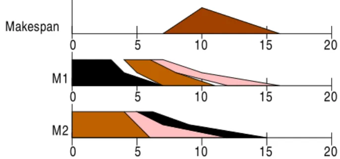
Let us illustrate the previous definitions with an ex-ample. Consider a problem of 3 jobs and 2 machines with the following matrices for fuzzy processing times and machine allocation:
ξ= (3,4,7) (1,2,3) (4,5,6) (2,3,4) (1,2,6) (1,2,4) ν= 1 2 2 1 2 1
For instance, ξ22 = (2,3,4) is the processing time of task 2 of job 2 θ22 and, given that ν22 = 1, this task must be processed on machine 1. Figure 1 shows the Gantt chart (adapted to TFNs) of the schedule given by the decision variable x=(1 2 3 2 3 1). It represents the partial schedules obtained from the decision vari-able for each machine. For machine 1, tasks are pro-cessed in the following order:θ11, θ22, θ32, and for ma-chine 2, tasks are processed in the order θ21, θ31, θ12. Given these orderings and precedence constraints, the starting time for taskθ22 will be the maximum of the completion times ofθ21 andθ11, the preceding tasks in the job and in the machine:S22=C21tC11= (4,5,6)t (3,4,7) = (4,5,7). Consequently, its completion time will beC22=S22+ξ22= (4,5,7) + (2,3,4) = (6,8,11). 5 10 15 20 0 5 10 15 20 0 5 10 15 20 0 Makespan M1 M2
Fig. 1 Gantt chart of the schedule represented by the deci-sion variable (1 2 3 2 3 1)
Notice that if uncertain durations are given as fuzzy intervals the scheduleswill be a fuzzy schedule, in the sense that the starting and completion times of all tasks and the makespan are fuzzy intervals. These fuzzy in-tervals may be seen as possibility distributions on the values that these times may take. However, the task processing ordering represented by x that determines such schedule is crisp; there is no uncertainty regarding the order in which tasks are to be processed. In other words, we obtain a fuzzy schedule from a crisp task ordering. These ideas are essential for the semantics of fuzzy schedules proposed in (Gonz´alez Rodr´ıguez et al., 2008) and described in Section 3.3.
3.2 Multiobjective Models
It is not trivial to optimise a schedule in terms of a
fuzzy quantity, since neither the maximum ∨ nor its
approximationt define a total ordering. In the litera-ture, this problem is tackled using some ranking method for fuzzy numbers, comparisons based onλ-cuts or de-fuzzification methods. Here the modelling philosophy is similar to that of stochastic scheduling and is inspired
A Genetic Solution based on Lexicographical Goal Programming for a Multiobjective Job Shop with Uncertainty 5
in the work on expected value models from (Liu and Liu, 2002).
If we only consider the makespan, the expected value
E[Cmax(x,ξ,ν)] should be minimised, thus providing
anexpected makespan modelfor fuzzy job shop (Gonz´alez Rodr´ıguez et al., 2007b). Similarly, we may define the
expected tardiness and theexpected idleness models or, in general, an expected model for any single fuzzy goal. Alternatively, we may consider several objectives and formulate a multiobjective problem. Now, with mul-tiple goals it is often the case that some are achievable only at the expense of others, hence the need of a hier-archy of importance among these possibly incompatible goals so as to satisfy as many as possible in the speci-fied order. In general, for k objectives f1, . . . , fk such
priority structure should be established by the deci-sion maker (DM) and may be represented by a one-to-one mapping ρ from {f1, . . . , fk} onto {1, . . . , k},
such that ρ(fi) is the priority level of fi, i= 1, . . . , k, where 1 represents the highest priority. For instance, if
f1=Cmax, f2=Tmaxandf3=Imaxand the DM
con-siders that the most prioritary objective is minimising the expected tardiness, then ρ(f2) = 1. Without loss of generality, let us assume that the objective functions
fi i = 1, . . . , k are ordered according to their priority, that is, ρ(fi) =i. Then, we may formulate the follow-ingexpected multiobjective model for the fuzzy job shop problem (FJSP): lexmin (E[f1(x,ξ,ν)], . . . , E[fk(x,ξ,ν)]) subject to: 1≤xl≤n, l= 1, . . . , nm, |{xl:xl=i}|=m, i= 1, . . . , n, xl∈Z+, l= 1, . . . , nm. (18)
where lexmin denotes lexicographically minimising the objective vector.
Additionally, a goal programming model may be used to balance the multiple conflicting objectives, con-sidering target levels established by the DM, soE[fi(x,ξ,ν)] should not exceed a given target value bi,i= 1, . . . , k. This translates into the following goal constraints:
E[fi(x,ξ,ν)] +d−i −d+i =bi, i= 1, . . . , k (19)
whered+i , the positive deviation from the target, should
be minimised. We thus obtain the following expected
fuzzy goal multiobjective model for the FJSP:
lexmin (d+1, . . . , d+k) subject to: E[fi(x,ξ,ν)] +d−i −d + i =bi, i= 1, . . . , k, bi, d−i , d+i ≥0, i= 1, . . . , k, 1≤xl≤n, l= 1, . . . , nm, |{xl:xl=i}|=m, i= 1, . . . , n, xl∈Z+, l= 1, . . . , nm. (20) Notice that (18) is a particular case of (20). Indeed, this last formulation is general enough to comprise all pos-sible fuzzy goals, priority structures and target levels established by the DM. Similar ideas for the fuzzy par-allel machine scheduling problem with a fixed priority structure and three objectives can be found in (Peng and Liu, 2004).
3.3 A-Posteriori Semantics of Fuzzy Schedules
In (Gonz´alez Rodr´ıguez et al., 2008), a semantics for the fuzzy schedules was proposed and used to measure the performance of such schedules. According to this semantics, solutions to the FJSP are interpreted as a-priori solutions, found when the duration of tasks is not exactly known. In this setting, it is impossible to predict what the exact time-schedule will be, because it depends on the realisation of the task’s durations, which is not known yet. Each schedule corresponds to a crisp ordering of tasks and, it is not until tasks are executed according to this ordering that we know their real duration and, hence, obtain a real schedule, the a-posteriori solutionwith crisp job completion times and makespan.
Given this, the main interest of a solution to the FJSP lies in the ordering of tasks that it provides a pri-ori, when information about the problem is incomplete. Ideally, this ordering should yield good schedules in the moment of its practical use, when tasks do have real durations. Hence, its behaviour should be evaluated on a family ofN crisp job shop problems, generated from the fuzzy problem so that they can be interpreted as its realisations. Such possible realisations are simulated by generating exact durations for each task at random according to a probability distribution which is coher-ent with the possibility distribution given by the fuzzy duration.
Given a solution to the FJSP, we consider the or-dering of tasks it provides, represented by the
deci-sion variable x. For a crisp version of the FJSP, let η be the matrix of crisp durations, such thatηij, the
a-posteriori duration of task θij is coherent with the possibility distribution defined by the fuzzy duration
ξij. Then, the orderingxcan be used by an algorithm
of semiactive schedule building to obtain a crisp time-schedule, as presented in Section 3.1 but using real du-rations instead of fuzzy ones. For such crisp schedule, the Relative Makespan Error, M E, is defined as the relative difference in time units between the obtained crisp makespanCmax(x,η,ν) and a given lower bound for the makespanLB(η,ν), that is:
M E(x,η,ν) = Cmax(x,η,ν)−LB(η,ν)
LB(η,ν) (21)
This lower bound may be obtained with some of the existing methods from the literature. We also define the
Feasibility Error, F(x,η,ν), as the proportion of due-date constraints that do not hold for a given orderingx for a given a-posteriori realisationη of task durations. If instead of a single crisp instance we consider the
whole family of N crisp problems, each with a
dura-tion matrix ηl, we obtain N values of M E, denoted
M El = M E(x,ηl,ν), and N values of F, denoted
Fl=F(x,ηl,ν),l= 1, . . . , N. The overall performance
of the fuzzy solution across the family ofN crisp prob-lems is then measured by the following average values:
M E(x) = PN l=1M El N , F(x) = PN l=1Fl N (22)
We may now compare different solutions to the FJSP based on due-date satisfaction (using F(x)), based on makespan (using M E(x)) or even based on the over-all achievement of both objectives (using some combi-nation of F(x) and M E(x)). In any case, we should bear in mind the quality of a given orderingxis mea-sured on a family of problems which may be quite di-verse. In fact, the greater the uncertainty in the FJSP, the greater the variety of possible crisp realisations and hence, the diversity within the family of associated crisp JSSPs.
4 Using Genetic Algorithms to Solve FJSP
The crisp job shop problem is a paradigm of constraint satisfaction problem and has been approached using many heuristic techniques. In particular, genetic algo-rithms (GAs) have proved to be a promising solving method (Bierwirth, 1995), (Mattfeld, 1995), (Varela et al., 2003).
The structure of a GA for the FJSP is described in Algorithm 2. First, the initial population is generated
and evaluated. Then the GA iterates for a number of generations. In each iteration, a new population is built from the previous one by applying the genetic operators of selection, recombination and acceptation.
Require: an instance of fuzzy JSP,P
Ensure: a schedulesforP
1. Generate the initial population; 2. Evaluate the population;
whileNo termination criterion is satisfieddo
3. Select chromosomes from the current population; 4. Apply recombination to the selected chromosomes to generate new ones;
5. Evaluate the chromosomes generated at step 4; 6. Apply the acceptance criterion to the set of chromo-somes selected at step 3 together with the chromochromo-somes generated at step 4;
returnthe schedule from the best chromosome evaluated so far;
Fig. 2 Genetic Algorithm
To codify chromosomes we use the decision vari-ablex, a permutation with repetition, which presents a number of interesting characteristics (Varela et al., 2005). The quality of a chromosome is evaluated by the fitness function, which is taken to be the objective function lexmin(d+1, . . . , d+k) as defined in (20).
In the selection phase, chromosomes are grouped into pairs at random. Each of these pairs is mated to obtain two offsprings and acceptance consists in select-ing the best individuals from the set formed by the pair of parents and their offsprings. For chromosome mating we consider theJob Order Crossover(JOX) (Bierwirth, 1995). Given two parents, JOX selects a random sub-set of jobs, copies their genes to the offspring in the same positions as they appear in the first parent, and the remaining genes are taken from the second parent so as to maintain their relative ordering. This operator has an implicit mutation effect. Therefore, no explicit mutation operator is actually necessary and parameter setting is considerably simplified, as crossover probabil-ity is 1 and mutation probabilprobabil-ity need not be specified. From a given decision variablexas explained in Sec-tion 3 we may obtain asemi-active schedule, meaning that for any operation to start earlier, the relative or-dering of at least two tasks must be swapped. However, other possibilities may be considered. For the crisp job shop, it is common to use the G&T algorithm (Gif-fler and Thomson, 1960), which is an active schedule builder. A schedule isactiveif one task must be delayed for any other one to start earlier. Active schedules are good in average and, most importantly, the space of ac-tive schedules contains at least an optimal one, that is, the set of active schedules isdominant (cf. (Brucker and
A Genetic Solution based on Lexicographical Goal Programming for a Multiobjective Job Shop with Uncertainty 7 Require: a chromosomexand a fuzzy JSPP
Ensure: the schedulesgiven by chromosomexfor problem
P
1: A={θi1, i= 1, . . . , n};/*set of first tasks of all jobs*/
2: whileA6=∅do
3: Determine the taskθ0∈Awith minimum earliest com-pletion timeC1
θ0 if scheduled in the current state;
4: LetM0 be the machine required by θ0 andB⊆Athe subset of tasks requiring machineM0;
5: Remove fromBany task θthat starts later thanCθ0:
Ci
θ0≤Sθi,i= 1,2,3;
6: Selectθ?∈Bsuch that it is the leftmost operation in
the sequencex;
7: Scheduleθ∗as early as possible to build a partial sched-ule;
8: Remove θ? fromAand insert inAthe task following
θ?in the job ifθ?is not the last task of its job;
9: returnthe built schedule;
Fig. 3 Extended G&T for triangular fuzzy times
Knust, 2006)). For these reasons it is worth to restrict the search to this space. Moreover, the G&T algorithm is complete for the job shop problem.
In Algorithm 1 we propose an extension of G&T to the case of fuzzy processing times. It should be noted nonetheless that with uncertain durations we cannot guarantee that the produced schedule will indeed be active when it is actually performed (and tasks have exact durations). We may only say that the obtained fuzzy schedule ispossibly active.
It often happens that a sequence of tasks is not com-patible in order to obtain an active schedule, so the de-coding algorithm in Algorithm 1 has to exchange the order of some tasks. This new order is translated to the chromosome, for it to be passed onto subsequent offsprings, thus GA exploiting the so-called lamarck-ian evolution. Again, an implicit mutation effect is ob-tained.
The GA described above has been successfully used in (Gonz´alez Rodr´ıguez et al., 2007b) for a single objec-tive job shop to minimise the expected makespan using semi-active schedules, comparing favourably to a simu-lated annealing algorithm from the literature (Fortemps, 1997). Also the GA combined with the extended G&T improves the expected makespan results obtained by a niche-based GA that follows the scheme proposed in (Sakawa and Kubota, 2000) with matrices of com-pletion times as chromosomes and recombination oper-ators based on fuzzy G&T.
5 Experimental Results
For the experimental results, we follow (Fortemps, 1997) and generate a set of fuzzy problem instances from
well-known benchmark problems: FT06 of size 6×6 and
LA11, LA12, LA13 and LA14 of size 20×5. This will al-low for comparisons with the simulated annealing (SA) algorithm proposed in that paper. From a given crisp processing time x, a symmetric fuzzy processing time
p(x) is generated as follows: the modal value isp2=x andp1,p3 are random values, symmetric w.r.t.p2 and generated so the TFN’s maximum range of fuzziness is 30% ofp2. To generate due dates, we use a method proposed in (Gonz´alez Rodr´ıguez et al., 2006). For job
Ji, let ιi = Pm
j=1p2ij be the sum of most typical
du-rations across all its tasks, for a given task θij, let
ρij =Pr6=i,s=6 j:νrs=νijp
2
r,s be the sum of most typical
durations of all other tasks requiring the same machine as θij, and let ρi = maxj=1,...,mρij be the maximum
of such values across all tasks in jobJi. Then, the due
date Di is a random value from [ιi+ 0.5ρi, ιi+ρi]. In total, 10 instances of fuzzy job shop are generated from each original benchmark problem.
Given the three fuzzy goals f1 =Cmax, f2 =Tmax and f3 = Imax, we consider five objective functions: three single-objective functions given by the expected values E[f1], E[f2] and E[f3] and two multiobjective functions that result from incorporating two different priority structures in expression (20). The first multi-objective functionl123corresponds to the priority struc-ture defined byρ(i) =i, that is, the most prioritary goal is the makespanf1, then the tardiness f2 and, finally, the idlenessf3. The second objective functionl213 cor-responds to ρ(f1) = 2, ρ(f2) = 1, ρ(f3) = 3, i.e. the most prioritary goal is to minimise tardiness, and the makespan becomes the second goal. These hierarchies correspond to probably the most common objectives in the job shop literature, namely minimise makespan or maximise due-date satisfaction.
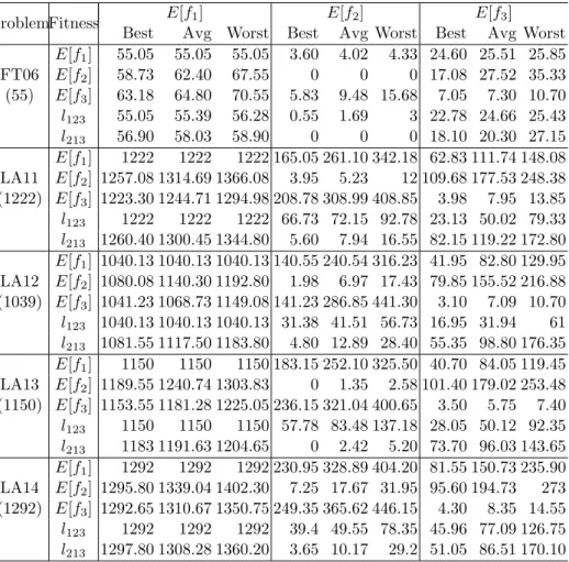
For each problem instance and objective function, the GA is run 30 times with population size 100 for 200 generations. To fix the target valueb1for the expected makespan, we use the experience gained usingE[f1] as single objective and set b1 equal to the average value of E[f1] across 30 runs of the GA. Target values for expected tardiness and idleness are in all cases b2 = b3= 0. Table 1 shows a summary of the results: for each fitness function we measureE[f1], E[f2] andE[f3] for the obtained schedule and compute the best, average and worst of these values across the 30 executions of the GA and the 10 problem instances generated from the same original problem. The optimal makespan value for the original crisp problem is also shown between brackets, as it provides a lower bound for the expected makespan of the fuzzified version (Fortemps, 1997).
From the results in Table 1, it is clear that the multiobjective versions with l123 and l213 behave sim-ilarly to the corresponding single-objective ones,E[f1]
Table 1 Results obtained by the GA
ProblemFitness E[f1] E[f2] E[f3]
Best Avg Worst Best Avg Worst Best Avg Worst
E[f1] 55.05 55.05 55.05 3.60 4.02 4.33 24.60 25.51 25.85 FT06 E[f2] 58.73 62.40 67.55 0 0 0 17.08 27.52 35.33 (55) E[f3] 63.18 64.80 70.55 5.83 9.48 15.68 7.05 7.30 10.70 l123 55.05 55.39 56.28 0.55 1.69 3 22.78 24.66 25.43 l213 56.90 58.03 58.90 0 0 0 18.10 20.30 27.15 E[f1] 1222 1222 1222 165.05 261.10 342.18 62.83 111.74 148.08 LA11 E[f2] 1257.08 1314.69 1366.08 3.95 5.23 12 109.68 177.53 248.38 (1222) E[f3] 1223.30 1244.71 1294.98 208.78 308.99 408.85 3.98 7.95 13.85 l123 1222 1222 1222 66.73 72.15 92.78 23.13 50.02 79.33 l213 1260.40 1300.45 1344.80 5.60 7.94 16.55 82.15 119.22 172.80 E[f1] 1040.13 1040.13 1040.13 140.55 240.54 316.23 41.95 82.80 129.95 LA12 E[f2] 1080.08 1140.30 1192.80 1.98 6.97 17.43 79.85 155.52 216.88 (1039) E[f3] 1041.23 1068.73 1149.08 141.23 286.85 441.30 3.10 7.09 10.70 l123 1040.13 1040.13 1040.13 31.38 41.51 56.73 16.95 31.94 61 l213 1081.55 1117.50 1183.80 4.80 12.89 28.40 55.35 98.80 176.35 E[f1] 1150 1150 1150 183.15 252.10 325.50 40.70 84.05 119.45 LA13 E[f2] 1189.55 1240.74 1303.83 0 1.35 2.58 101.40 179.02 253.48 (1150) E[f3] 1153.55 1181.28 1225.05 236.15 321.04 400.65 3.50 5.75 7.40 l123 1150 1150 1150 57.78 83.48 137.18 28.05 50.12 92.35 l213 1183 1191.63 1204.65 0 2.42 5.20 73.70 96.03 143.65 E[f1] 1292 1292 1292 230.95 328.89 404.20 81.55 150.73 235.90 LA14 E[f2] 1295.80 1339.04 1402.30 7.25 17.67 31.95 95.60 194.73 273 (1292) E[f3] 1292.65 1310.67 1350.75 249.35 365.62 446.15 4.30 8.35 14.55 l123 1292 1292 1292 39.4 49.55 78.35 45.96 77.09 126.75 l213 1297.80 1308.28 1360.20 3.65 10.17 29.2 51.05 86.51 170.10
andE[f2], regarding their most prioritary goal. Besides, they improve considerably on the remaining goals. In-deed, l123 and E[f1] obtain identical makespan values in all problem instances except those stemming from FT06, where the relative difference with respect to the expected makespan lower bound (55) is less than 1% in average. The expected tardiness values withl123are better than withE[f1] in all cases. Clearly, minimising the makespan does not always imply minimising tar-diness. If we consider the relative values ofE[f2] with respect to the lower bound of the expected makespan (as a means of comparing tardiness values across dif-ferent problem instances) we see that l123 obtains an average reduction of 4.24% in FT06 instances and of 17.73% in LA problem instances. Regarding expected idleness, l123 improves in average 1.55% for FT06 in-stances and 4.65% for LA inin-stances (again, relative to the lower bound for the expected makespan). If we com-parel213 toE[f2], expected tardiness is equal for FT06 instances and only 0.8% worse in average for LA in-stances, while expected makespan improves in average 7.94% and 2.5% for FT06 and LA instances
respec-tively. Expected idleness also improves in both fami-lies, with values 13.13% and 6.46% better in average. This illustrates that, despite being the last goal, Imax
is indeed taken into consideration in the optimisation process when l123 and l213 are used. Of course, being the last prioritary goal in both cases, it is natural that the expected idleness values forl123andl213 are not as good as those obtained withE[f3].
Notice that the expected tardiness improvement for
l123 is greater in LA problems than in FT06 instances. This is not surprising since tardiness values obtained withE[f1] for FT06 are already close to target values. This is not the case for LA instances, where there is greater room for improvement. The same explanation
holds for makespan improvement when using l213
in-stead ofE[f2], which is greater for FT06 instances than for LA ones. Notice as well that comparisons between different multiobjective functions do not make sense, as they model different priority requirements.
Let us now compare the GA using l123 with the
single-objective SA algorithm from (Fortemps, 1997). In that work, 10 problem instances were also
gener-A Genetic Solution based on Lexicographical Goal Programming for a Multiobjective Job Shop with Uncertainty 9
Table 2 Comparison of results forE[Cmax]
Problem E[f1] and SA l123 and GA
Best Avg Worst Best Avg Worst
FT06 55.02 55.2 56.01 55 55.05 55.25
LA11 1222 1222 1222 1222 1222 1222
LA12 1041 1046.81 1056.35 1039 1040.13 1043.25
LA13 1150 1155.07 1181.76 1150 1150 1150
LA14 1292 1292 1292 1292 1292 1292
ated from the same original benchmark problems with the same method but using 6-point fuzzy intervals, a particular case of which are TFNs. Table 2 contains expected makespan results for both methods. It shows the best, average and worst solutions obtained by the GA with l123 across the 10 instances generated from the same crisp problem, together with the results re-ported in (Fortemps, 1997). In Section 4 we already mentioned that the GA optimising onlyE[Cmax]
com-pared favourably with the SA algorithm. Table 2 shows that this is also the case for the multiobjective function
l123with makespan as its most prioritary goal.
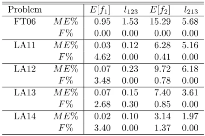
Table 3 Results for the a-posteriori semantics
Problem E[f1] l123 E[f2] l213 FT06 M E% 0.95 1.53 15.29 5.68 F% 0.00 0.00 0.00 0.00 LA11 M E% 0.03 0.12 6.28 5.16 F% 4.62 0.00 0.41 0.00 LA12 M E% 0.07 0.23 9.72 6.18 F% 3.48 0.00 0.78 0.00 LA13 M E% 0.07 0.15 7.40 3.61 F% 2.68 0.30 0.85 0.00 LA14 M E% 0.02 0.10 3.14 1.97 F% 3.40 0.00 1.37 0.00
Finally, Table 3 presents the obtained values of the performance measuresM EandFbased on the a-posteriori semantics presented in Section 3.3. They are average values across the 10 problems of a same family, rescaled as percentage values, obtained with different objective functions: two single-objective functions corresponding to makespan and tardiness and the two multiobjective functionsl123andl213where the most prioritary goal is, respectively, the makespan and the tardiness. The re-sults for the a-posteriori semantics, i.e., the behaviour of the task processing order on possible realisations of task durations, coincide with the results for the ex-pected objective values in Table 1 and further support the corresponding analysis: the multiobjective versions withl123andl213behave similarly to the corresponding
single-objective ones,E[f1] and E[f2], regarding their most prioritary goal, whilst improving on the secondary goal. If we compare the multiobjective functionl123 to E[f1], we see that theM Eincreases in average less than 0.2%, whilst F is considerably reduced. In fact,F be-comes null in all cases except LA13, where it goes from 2.68% al 0.3%. Comparingl213 to E[f2], the multiob-jective version clearly outperforms the single obmultiob-jective one: not only do relative makespan errorsM E improve considerably (up to 10%), but due-date fulfilment is also better or equal in all cases. In fact, in all cases but one the a-posteriori schedules obtained with multiobjective optimisation fully satisfy the due dates. There seems to be a clear synergy effect among different goals in the multiobjective approach.
6 Conclusions and Future Work
We have considered a job shop problem with uncertain durations. Such uncertainty is modelled using TFNs and the goal is to find a task processing order that yields a feasible schedule optimising several objectives, for in-stance, fuzzy makespan, fuzzy tardiness and fuzzy idle-ness. We have proposed to formulate the multiobjective problem as a fuzzy goal programming model according to a generic priority structure and target levels estab-lished by the decision maker, using the expected value of the fuzzy quantities. As solving method, a GA with codification based on permutations with repetitions has been described. Experimental results on fuzzy versions of well-known crisp problem instances illustrate the po-tential of both the proposed multiobjective formulation and the GA. This is further illustrated with experi-mental results that incorporate the semantics of fuzzy schedules proposed in (Gonz´alez Rodr´ıguez et al., 2008) In the future, the multiobjective approach will be further analysed using a more varied set of problem in-stances. This wider set of problems should also enable a thorough parametric analysis of the target values estab-lished by the decision maker. Finally, the GA may be hybridised with other heuristic techniques, such as local
search, to increase its potential. This leads to further studying task criticality for fuzzy durations.
Acknowledgements
All authors are supported by MEC-FEDER Grant TIN2007-67466-C02-01. A preliminary version of this work was presented at the Workshop on Planning, Scheduling and Constraint Satisfaction held in conjunction with CAEPIA 2007 (Gonz´alez Rodr´ıguez et al., 2007a).
References
Bierwirth, C. (1995). A generalized permutation ap-proach to jobshop scheduling with genetic algo-rithms. OR Spectrum, 17:87–92.
Brucker, P. and Knust, S. (2006). Complex Scheduling. Springer.
Dubois, D., Fargier, H., and Fortemps, P. (2003a). Fuzzy scheduling: Modelling flexible constraints vs.
coping with incomplete knowledge. European
Jour-nal of OperatioJour-nal Research, 147:231–252.
Dubois, D., Fargier, H., and Galvagnon, V. (2003b). On latest starting times and floats in activity networks with ill-known durations. European Journal of Oper-ational Research, 147:266–280.
Dubois, D., Fargier, H., and Prade, H. (1996). Possibil-ity theory in constraint satisfaction problems: Han-dling priority, preference and uncertainty. Applied Intelligence, 6:287–309.
Dubois, D. and Prade, H. (1988). Possibility Theory: An Approach to Computerized Processing of Uncer-tainty. Plenum Press, New York (USA).
Fayad, C. and Petrovic, S. (2005). A fuzzy genetic al-gorithm for real-world job-shop scheduling. Innova-tions in Applied Artificial Intelligence, Lecture Notes in Computer Science, 3533:524–533.
Fortemps, P. (1997). Jobshop scheduling with imprecise
durations: a fuzzy approach. IEEE Transactions of
Fuzzy Systems, 7:557–569.
Fortemps, P. and Roubens, M. (1996). Ranking and defuzzification methods based on area compensation.
Fuzzy Sets and Systems, 82:319–330.
Giffler, B. and Thomson, G. L. (1960). Algorithms for solving production scheduling problems. Operations Research, 8:487–503.
Gonz´alez Rodr´ıguez, I., Puente, J., Vela, C. R., and
Varela, R. (2008). Semantics of schedules for the
fuzzy job shop problem. IEEE Transactions on
Sys-tems, Man and Cybernetics, Part A. Accepted for publication.
Gonz´alez Rodr´ıguez, I., Vela, C. R., and Puente, J. (2006). Study of objective functions in fuzzy job-shop
problem. ICAISC 2006, Lecture Notes in Artificial
Intelligence, 4029:360–369.
Gonz´alez Rodr´ıguez, I., Vela, C. R., and Puente, J. (2007a). A genetic solution for multiobjective fuzzy job shop based on lexicographical goal program-ming. In Salido, M. A. and Fdez-Olivares, J., ed-itors, Proc. of the Workshop on Planning, Schedul-ing and Constraint Satisfaction, pages 93–104, Sala-manca (Spain).
Gonz´alez Rodr´ıguez, I., Vela, C. R., and Puente, J.
(2007b). A memetic approach to fuzzy job shop
based on expectation model. InProceedings of IEEE International Conference on Fuzzy Systems, FUZZ-IEEE2007, pages 692–697, London.
Liu, B. (2006). A survey of credibility theory. Fuzzy Optimization and Decision Making, 5:387–408. Liu, B. and Liu, Y. K. (2002). Expected value of fuzzy
variable and fuzzy expected value models. IEEE
Transactions on Fuzzy Systems, 10:445–450.
Mattfeld, D. C. (1995). Evolutionary Search and the
Job Shop Investigations on Genetic Algorithms for Production Scheduling. Springer-Verlag.
Peng, J. and Liu, B. (2004). Parallel machine schedul-ing models with fuzzy processschedul-ing times. Information Sciences, 166:49–66.
Sakawa, M. and Kubota, R. (2000). Fuzzy program-ming for multiobjective job shop scheduling with fuzzy processing time and fuzzy duedate through
ge-netic algorithms. European Journal of Operational
Research, 120:393–407.
S lowi´nski, R. and Hapke, M., editors (2000).Scheduling Under Fuzziness, volume 37 of Studies in Fuzziness and Soft Computing. Physica-Verlag.
Varela, R., Serrano, D., and Sierra, M. (2005). New codification schemas for scheduling with genetic algo-rithms.Lecture Notes in Computer Science, 3562:11– 20.
Varela, R., Vela, C. R., Puente, J., and G´omez, A.
(2003). A knowledge-based evolutionary strategy
for scheduling problems with bottlenecks. European Journal of Operational Research, 145:57–71.
Yager, R. R. (1981). A procedure for ordering fuzzy subsets of the unit interval. Information Sciences, 24:143–161.