Uncertain volatility pricing in QuantLib

(1)

Title: Uncertain Volatility in QuantLib

Author: Carles Jou

Advisor: Josep J. Masdemont

Department: Matemàtica Aplicada 1

Academic year: 2009

(2)

U

niversitat

P

olit

ecnica de

`

C

atalunya

M

aster en

E

nginyeria

M

atem

atica

`

U

ncertain

V

olatility

P

ricing in

Q

uant

L

ib

Master Project Dissertation

by C

arles

J

ou

Advisor: Josep J. Masdemont

June 2009

(3)

(4)

Abstract

Quantitative finance has acquired a significant role in the markets during the past years with financial institutions increasingly hiring scientists, so-called quants, to discover pat-terns or relationships in prices and to implement strategies to exploit them.

One area with significant quants presence is derivative pricing. In this domain, the main goal is to consistently evaluate different instruments that depend on the same sources of risk. With this purpose, models of the risk sources are elaborated and arbitrage pric-ing theory is used to determine prices and replicatpric-ing strategies. However, as far as the modelled risk is controlled and measurable, the risks associated to the specification of the model remain important and out of its scope. For the most widely used model class, diffusion models, we observe a significant dependency on the volatility parameter. On the theoretical side, this project is focused on the study of an extension of diffusion models that integrates the volatility risk: the uncertain volatility model [ALP95]. In this model, the volatility parameter is no longer specified as a single value but as an interval. From this volatility interval, an interval for the derivative price is determined. The price envelope gives a consistent and reliable quantitative measure of the volatility exposure. A relevant feature of the model is that, in presence of changing convexity, the pricing equa-tion becomes non-linear, making the valuaequa-tion portfolio-dependent.

On the practical side, the aim of the project is to introduce QuantLib, an open source C++ library for quantitative finance and use it in the implementation of the uncertain volatility model. Given the (provisional) lack of official support documentation, an introduction to the structure and main features of QuantLib has been elaborated. The functioning of the library is illustrated with the integration of Uncertain Volatility pricing functionalities and their use in applications.

(5)

As a whole, the goal of the project is to provide an overview of the techniques and tools used in derivatives pricing and illustrate all the stages of a project in this field: from the generation of a theoretical model, to its implementation in pricing applications.

(6)

Chapter 1

Introduction

1.1 Motivation

Capitalist economies rely on capital markets as meeting points between financial resources and projects. Since the outcomes of the projects remain uncertain, capital holders will re-quire their investments to be remunerated according to their risk-taking. Efficient capital markets should match the risk profile of investors and the projects in the market. To ar-ticulate this market of risk, financial securities provide at a certain price the rights over a share of the returns of a project. The valuation of these financial instruments will then be critical: in primary markets, it will determine the funding capabilities for new projects whereas in secondary markets it will adjust the risk allocation according to the informa-tion flow. To make the capital markets more dynamic and in some way more efficient, financial intermediaries issue new and more complex financial securities to adapt the ex-isting projects to investors risk profiles.

In general, the evaluation of financial securities will not be objective in that it will heavily rely on the risk appreciation by the potential buyer. However, there is one particular class of financial securities that can be consistently valued and whose price can be enforced by arbitrage mechanisms, that is, potentially unlimited risk-less profits are possible until the price converges to its natural value. These are derivative securities: securities whose value depends on the price of a specified underlying. The idea is simple: we have only one source of risk and two traded securities depending on it; since their value should only depend on that same source of risk, they should be somehow related. Otherwise, one

(9)

could exploit this incoherence by buying at a low price, repackaging the risk at no cost and selling it at a higher price.

Derivative instruments have grown in importance in the last decades because they allow tailor-made products that fit the needs of asset managers and fund allocators. The issuers and traders of such products will need to evaluate them accurately so that no free money is given away by mispricing. At this point, the industry heavily relies on mathematical models mostly coming from the work of Black and Scholes. Generally these models make some assumptions on the behaviour of the underlying and then consistently price a set of securities depending on that underlying. Their main feature is that they provide hedging strategies to enforce a (range of ) price. However, valuation is far from being a risk-less business and the inability of models to fully capture reality generates an additional risk. In this context, the mission of financial institutions will be to package the risk, evaluate and hedge it in a particular framework, and take speculative positions with respect to the residual unhedgeable risks. To handle the complexity of the models, financial insti-tutions heavily rely on information technologies. The growth of computing capabilities has boosted the size derivatives markets.

1.2 Aim and organization of the project

The aim of this project is to focus on a particular class of valuation models and study it both from a theoretical and from a practical point of view.

The first part of the dissertation focusses on the basics of securities pricing and particu-larly on derivatives pricing and hedging. In this part we will identify the main sources of risk and distinguish hedgeable and unhedgeable risk, particularly in the context of diffu-sion models.

Since volatility turns out to be the critical parameter that conveys most of the specifica-tion risk, special attenspecifica-tion will be devoted to its modelling in the chapter 3 and we will particularly focus on a model that integrates part of this risk in the prices: the uncertain volatility model by Avellaneda, Levy and Paras.

For the practical side, we will explore an open source solution, QuantLib, very promising in terms of its functionalities and potential for the future of the industry. In particular,

(10)

1.2 Aim and organization of the project 3

chapter 4 will focus on the motivations and design of the library.

Finally, in chapter 5, we implement the model presented in the previous sections as a QuantLib module and test some applications of the model.

(11)

(12)

Chapter 2

Background

2.1 Securities pricing overview and modelling philosophy

Our first aim is to provide a framework to evaluate investments. According to basic fi-nancial theory, the main postulate for investment valuation is that the present value of an investment should be calculated as the sum of its future cash flows, discounted at a certain rate dependent on the time at which they occur. The discounting process conveys the opportunity cost of other investments such as cash deposits or, otherwise, a relative valuation of risk; for simplicity, we will present a basic modelling framework omitting this feature. The main issue remains that the future cash flows may be uncertain. We should

then move toexpectedcash flows. We will need an estimate of possible future scenarios

and a suitable measure over these scenarios to validly compute the expectations. But what future scenarios will we consider? What do we mean by a suitable measure? This is where models come in.

The key point in securities pricing theory is to assume that market prices contain all known information about the future and that markets are efficient in that the prices are deter-mined so as to make any systematic profit impossible. This Efficient Market Hypothesis could be restated as follows: market prices are the expected prices taking into account all the available information. The market is thus implicitly using a measure that contains all this information about the future. It is natural then to value any claim using this same measure. By doing so, the achieved valuation could only be outperformed by luck. From

(13)

this point of view, securities pricing is merely the recovery of a market measure.

But first things first. We are talking about measures but we first need a probability space, a set on which to establish a measure. The modelling task starts by specifying future sce-narios. But how will the future turn out? If asked about what will happen tomorrow, the first natural question should be: about what? A choice should be made about the drivers of uncertainty and how these may turn out. We may regard this uncertainty drivers as nat-ural state variables which determine future scenarios.

Next, one should be able to describe the price of traded securities, in each of the scenarios, deterministically from the state variables.

Once we have specified the future scenarios and the value of basic securities in each of them, we want to recover the measure that gives the present price as the sum of the ex-pected cash flows. In our simplified model, one could ask if such a measure will actually exist. It turns out that considering an arbitrage-free model will suffice to ensure the exis-tence of suitable pricing measures.

With the measures obtained we can price other securities by computing and adding their expected cash-flows over a time interval. We are implicitly assuming that future scenarios of the modelled securities will be relevant for the new securities we are pricing. This turns out to be especially true in the case of contingent claims, whose value depend on the val-ues of the underlyings and thus naturally share the set of future possible scenarios. The issue comes when we are left with various measures that fulfill the pricing requirements. These will be incomplete markets models as opposed to complete market models where only one measure satisfies the pricing requirements. In this situation, the best we can do is to provide a range for the price.

One of the most celebrated features of this whole pricing theory is that it provides hedging methods: the key point is that if the behaviour of different securities is known under dif-ferent scenarios then one can build a portfolio that replicates to some extent one security from the others. The more closely related securities are, the easier it is to achieve a good

(14)

2.2 Models and Fundamental Asset Pricing Theorem 7

hedge. Thus, modelling, as stated by Derman [Der96], will be about finding similar secu-rities to the ones we want to value. If the hedging is perfect, then the price can be enforced through arbitrage. Logically, a model will only provide a perfect hedge if it provides a sin-gle price. The converse is trivially true: if a model provides the means for a perfect hedge, then only one price will be admissible: the cost of the replicating strategy (this is the law of one price: two securities having the same payoffs must have the same initial value). So perfect hedging will be possible in and only in complete market models. In incomplete markets, we will be left with some additional risk. The different prices provided by the different measures can be understood as different ways to price this leftover risk.

In brief, a model should provide:

- a description of future scenarios according to some state variables, - the market price of traded assets in these scenarios,

- an effective way to recover the suitable measures in order to compute expectations, - an effective way to design hedging strategies.

2.2 Models and Fundamental Asset Pricing Theorem

We now turn to the mathematical formulation of such models.

Let ˜Ωbe the set of possible realizations of our world. Since this set is too abstract to work upon, the first idea is to restrict it through the use of a number of time dependent state variables whose evolution we can model. We first define a time intervalI⊂R+, either dis-crete or continuous. We then define ˜Xi: ˜Ω×I→Rto be our state processes,i=1..n. As we mentioned, we want to restrict our probability set to the behavior of our state variables, thus it is natural to define the following equivalence relationship: ˜ω≡_ω˜0_⇔ _X˜_i_{( ˜}_ω_,_t₎₌

˜

Xi( ˜ω0,t) for alli =1..n andt∈I. We finally defineΩ=Ω˜/≡as our working probability set. The state processesXiwill be naturally defined asXi:Ω×I→R, whereXi(ω)=X˜i( ˜ω),

˜

ωbeing one representative of theωclass. These new variables are well defined since the value of the state variable will not be dependent on the choice of the representative. We

(15)

note thatΩcan be thought of as the different paths the state variables can jointly follow.

Next thing to do is to describe the behaviour of these state variables under a given proba-bility. To do so, we will need a probability space, for which we need aσ-algebraF overΩ. Theσ-algebra models in some way the information that we may get from the realization of Ω. It is then natural to make thisσ-algebra time-dependent, as the more time elapses, the more able we will be to distinguish between different realizations. To model this feature, we will consider a filtration, that is, a sequence ofσ-algebras {Ft|t∈I} such thatFi⊆Fj fori ≤ j. The resulting (Ω,F,Fi) is a filtered probability space. We then can define a probabilityPon this space such that the distribution of the state variables is known.

Now that we have a grip on what our newly defined world is like, we turn to model the asset prices in the scenarios we just defined. For each traded asset, we will model its price through a stochastic process defined as a deterministic function of the state variables:

Sj=fj(X1, . . . ,Xn) forj=1..m. We note that sometimes we will be modelling other quan-tities, such as interest rates, and the derived asset prices will depend on this intermediate modelled variable.

If we turn to the recovery of the pricing measure, the first thing we should logically impose is that the new pricing measureQcan be used to retrieve the described pricing processes. This means that, at any time, their value can be computed as the expected future value with the known information. In mathematical terms: Sj(s)=EQ(Sj(t)|Fs) for alls≤t. This is the definition of martingales. So, for a measure to be acceptable to price securi-ties, we will ask it to make the modelled pricing processes martingales. In fact, here we have local martingales; to have proper martingales we should also impose the technical conditionE_Q(|Sj|)< ∞for all j=1..m. The measures that fulfil this requirement will be called martingale measures. In particular, we will be interested in equivalent martingale measures (EMM), those that preserve the views on possibility introduced by the original

measureP.

To find the pricing process for other claims, all we need to do is to find the expectation of their future value with respect to our pricing measures. If we denote byVt the pricing process for claimX, we have, for a given pricing measureQ,V_tQ=EQ(X|Ft).

(16)

2.2 Models and Fundamental Asset Pricing Theorem 9

Finally, to cover the last modelling requirement, we must talk about hedging. The key point here is the use of martingale representation results. General martingale theory pro-vides us with representation results for square integrable martingales. By considering the martingales set as a Hilbert space with a scalar product induced by the quadratic variation, one can represent a martingale in terms of a series of orthogonal martingales, with predictable coefficients with respect to the filtration. If the number of martingales needed to achieve the representation of the first martingale is finite, we then talk about the predictable representation property. Thus, in markets whose securities satisfy this ba-sic property, we will be capable to achieve perfect hedges. Otherwise, the finite number of securities will not allow us to completely reproduce the new security and so we will be left with an unhedgeable risk. It goes without saying that complete markets will satisfy the predictable representation property.

We close this section with the most important result in pricing theory: the Fundamental Asset Pricing Theorem that provides necessary and sufficient conditions for the existence and unicity of pricing measures (EMMs).

1. The market is arbitrage-free if and only if there is at least one EMM; and

2. in which case, the market is complete if and only if there is exactly one such EMM and no other.

An interesting remark is that for no arbitrage opportunities to exist, one must have at least as much independent securities as sources of uncertainty. On the other side, complete-ness requires the converse. So there will only be room for efficient complete market mod-els when the number of independent securities equals the number of sources of random-ness.

When it comes to the market practice, it is reasonable to assume that no arbitrage oppor-tunities exist, since if they existed, they would rapidly be materialized and disappear in the dynamics of the market. As for the completeness, there is empirical evidence that this condition does not hold[CGM01]. From the previous remark, this is quite reasonable as to properly model the behaviour of equities, one will need to introduce many sources of

(17)

ran-domness. Besides, another source of markets incompleteness is that trading strategies are limited: discrete trading and transaction costs stand against the completeness in practice.

To deal with market incompleteness, one can stick to Arbitrage Pricing Theory (APT) that we just described and that provides bounds for the prices (though generally this bounds will be insufficiently tight) or otherwise move to the expected utility maximization (EUM) framework, where the choice of the final pricing measure is made by optimizing a utility function of the investor (the drawback in this case is that the theory does not take into account the views of other market participants; besides, traders do not write down their utility function).

2.3 Diffusion models

The most popular class of models is the one that assumes that the state variables’ be-haviour can be modelled by diffusion processes.

The appeal of diffusion models comes from their analytical tractability and their use in the work of Black-Scholes and previously Bachelier for equity modelling.

The key feature of these models is their use of Brownian motion (or Wiener processes) to describe the randomness.

Definition: The processW =(Wt:t≥0) is aP-Brownian motion if and only if:

1. W0=0

2. Wt is almost surely continuous

3. Wthas independent increments withWt−Ws∼N(0,t−s) (for 0≤s<t).

Following the modelling agenda established in the previous sections, we start by definig our state processes: letW =(W1, . . . ,Wn) where theWi’s are independent Brownian

mo-tions. VectorW collects all the randomness of our model. By repeating the construction

(18)

2.3 Diffusion models 11

variables may jointly follow. Over this probability space, the Brownian motions are implic-itly defining a probability measure. This measure can be recovered using joint likelihood functions: suppose we take a time-mesh and we set the values of the variables at the times of the mesh. Then, since we know the distribution of each variable at each time, we can recover a joint likelihood for the variables to take such values. Taking the mesh to the limit, we can compute the likelihood of any possible path, which can be then extended to any set of paths. Thus, by saying that our state processes behave like Brownian motions, we are implicitly defining a whole probability space along with a measure which we will callP.

Next step in our construction is to describe the behaviour of the basic assets from the state variables. We will model their pricing processes as stochastic processes adapted to

then-dimensional brownian motion ofW.

Definition: A stochastic process adapted ton-dimensional Brownian motion

is a continuous processSt,t≥0, such thatStcan be written as

St=S0+ n X i=1 Z t 0 σi (s)dW_si+ Z t 0 µs d s,

whereσ1, . . . ,σn andµare randomF-previsible processes such that the in-tegralR₀t(P

iσ2_i(s)+ |µs|)d sis finite for all times t (with probability 1). The differential form of this equation can be written

d St= n

X

i=1

σi(t)dWti+µtd t.

Once we have the description of the behaviour of our basic assets, we turn to the specifica-tion of equivalent measures that make these price processes martingales. The Cameron-Martin-Girsanov (CMG) theorem plays a key role in this step as it provides an equivalence, up to technical conditions, between drift and measures. This result proves to be partic-ularly useful as one can characterize martingales in terms of the drift (martingales are driftless processes up to a technical condition on the quadratic variation). So the CMG theorem reduces the problem of finding suitable measures to the problem of finding the changes of measure that eliminate the drift. It provides us thus with an "effective way to recover the pricing measures".

Theorem (Cameron-Martin-Girsanov): LetW =(W1, . . . ,Wn) ben-dimensional

(19)

process which satisfies the general growth conditionE_Pexp(1₂RT

0 |γt|2d t< ∞,

and we set ˜W_ti =W_ti+R0tγisd s. Then there is a new measureQ, equivalent toPup to timeT, such that ˜W :=( ˜W1, . . . , ˜Wn) isn-dimensionalQ-Brownian motion up to timeT. The Radon-Nikodym derivative ofQwith respect toPis

dQ dP =exp ³ − n X i=1 Z T 0 γ i tdWti− 1 2 Z T 0 |γt| 2_{d t}´ .

The converse is also true. Since we want equivalent measuresQunder which all the

dis-counted asset prices areQ-martingales simultaneously, all we have to do is to find theγ that eliminates the drift in our processes. Then, we will be able to recover the correspon-dent pricing measure through the Radon-Nikodym derivative characterized in the CMG theorem.

The driftγwe have to add in this case must satisfy: n

X

i=1

σi j(t)γ_tj=µit, for allt,i=1, . . . ,n.

If we add here a discounting process with respect to a (riskless) security with driftrt and we require the discounted assets to be martingales, this amounts to impose on the assets processes to have the same drift as the numeraire security. In such case, the drift we have to add must satisfy:

n

X

i=1

σi j(t)γ_tj=µti−rt, for allt,i=1, . . . ,n,

or in matrix terms, where we defineΣtto be the matrix (σi j(t))i j:

Σtγt=µt−rt1.

This formulation is particularly interesting if one tries to draw some similarities with the Capital Asset Pricing Theory (CAPM): in this theory, risk is measured as variance and it has to be rewarded with returns over the riskless assets. The ratio between risk and reward is the market price of risk and is measured as the extra return over the riskless asset per variance unit. This is exactly the same formula we have obtained forγt (should it exist). It is then natural to callγtthe "market price of risk". If we push further this observation, we notice that once we make a change of measure,γt is fixed and so, every asset in the economy should become a martingale under the same change of measure (otherwise, the no-arbitrage condition would be violated). This amounts to say that all traded securities

(20)

2.3 Diffusion models 13

should have the same market price of risk in order to avoid arbitrage.

We must remark that the existence and unicity ofγt depend on the actual values of the

parametersΣt,µtandrt. The existence of several solutions for this equation is equivalent to having several pricing measures, that is, an incomplete market model. One could then say that the different prices that we can obtain correspond to the different prices of risk and so to the risk aversion of the investor. We note that ifΣt is invertible, then there is a uniqueγtand under the martingale measure,γt is zero; so the pricing measure is the one that has null market price of risk and so is known as risk-neutral.

Once we have the pricing measures, one can obtain the price by computing the expec-tations with this measure. The ability to obtain closed forms will mostly depend on the actual values of the model parameters. Later on, we provide a couple of examples.

We finally turn to the issue of hedging. Here, we focus on those market models where a complete hedge is possible, that is, those that satisfy the predictable representation prop-erty. This property can be stated as follows in the case of diffusion processes:

Theorem (Martingale representationn-factor):

Let ˜W ben-dimensionalQ-brownian motion, and suppose thatMt is ann -dimensionalQ-martingale process,Mt=(M1(t), . . . ,Mn(t)), which has volatil-ity matrix¡

σi j(t)¢, in thatd Mj(t)=Piσi j(t)dW˜i(t), and the matrix satisfies the additional condition that (with probability one) it is always non-singular. Then, ifNtis another one-dimensionalQ-martingale, there exists ann-dimensional

F-previsible processφt=(φ1(t), . . . ,φn(t)) such thatR₀T(Pσi jφj(t))2d t< ∞ with probability one andN can be written as

Nt=N0+

Z t

0 φs

d Ms.

Furthermore,φis (essentially) unique.

LetXbe a derivative maturing at timeTand letEtbe theQ-martingaleEt=EQ(BT−1X|Ft) andZt=Bt−1St. Here,Brepresents the discounting process mentioned in the introduc-tion. If the matrix Σt is always invertible, then the n-factor martingale representation

(21)

theorem gives us a volatility vector processφt=(φ1t, . . . ,φnt) such that Et=E0+ n X j=1 Z t 0 φ j sd Z j s.

The invertibility ofΣtis essential at this stage. Our hedging strategy will be (φ1t, . . . ,φnt,ψt) whereφi_t is the holding of securityi at timet andψt is the bond holding. As usual, the

bond holdingψis ψt=Et− n X j=1 φtjZ j t,

so that the value of the protfolio isVt=BtEt. The portfolio is self financing in that

dVt= n X j=1 φtjd S j t+ψtd Bt.

To summarize, we have seen that diffusion models are easily tractable. They depend ba-sically on two parameters: drifts and volatilities. One can look at these parameters as first and second order parameters. What we are doing in some way is letting the market fix the first order parameters (to make processes driftless) while we have a choice on the second order parameters. Since the measure changes to adjust the drift do not affect the volatility, pricing securities under diffusion models will be about speciying the volatities.

Examples

1) Black-Scholes

Probably the most famous example of diffusion processes is the Black-Scholes model for equities. In the simplest version of the model we have one source of uncertainty and one stock. The price process for the stock isd St=St(µd t+σdWt). With these assumptions, stock returns are normally distributed. The model’s first application was the valuation of contingent claims such as plain vanilla options for which it has proven to be extremenly successful. Under these assumptions, the model provides closed expressions for calls and puts whose popularity has grown to the extent that some products are quoted in terms of their implied volatility.

(22)

2.4 A complementary approach: PDE 15

2) Hull and White

This model applies diffusion processes to describe the evolution of interest rates. In par-ticular, it focusses on the evolution of the short rate, the interest for an instantaneous spot borrowing. One noticeable feature for this model is the mean reverting driftd rt = (θt−art)d t+σdWt. This short-rate process is assumed to be given under the risk-neutral measure. The price of bonds can be obtained by calculating forward rates so as to make arbitrage impossible and then integrating on these forward rates. Pricing of other interest rate contingent claims can be obtained in a similar fashion.

We close this section with an ouverture to other models. If we consider the family of prob-ability distributions that fulfill:

1. X0=0;

2. Xhas independent and stationary increments;

3. Xt+s−Xthas an infinitely divisible distribution.

If we take this distribution to be a normal, we obtain the browninan motion case we have just presented. We could have instead chosen any other distribution such as Poisson, Gamma, Inverse Gamma, CMY, . . . Distributions with fatter tails are becoming increas-ingly popular, especially in the field of credit derivatives.

2.4 A complementary approach: PDE

For diffusion models there exists one complementary approach for contingent claims pricing based on partial differential equations (PDEs). We present the one-factor case, as the extension to multi-factor is straightforward and only adds complexity to the formu-lae.

We begin by assuming that we have one basic assetS(the extension to several assets could be easily done, taking care that the no-arbitrage condition still holds) and that the

(23)

be-haviour of this asset is given by the following equation:

d St=µtd t+σtdWt (2.1)

Then, for a derivative securityZ, its behaviour can be written as follows (using Itô calcu-lus): d Zt = ∂ Zt ∂t d t+ ∂Zt ∂St d St+ 1 2 ∂2_Z t ∂S2 t (d St)2 = Ã ∂Zt ∂t +µt ∂Zt ∂St + 1 2σ 2 t ∂2_Z t ∂S2_t ! d t+σt∂ Zt ∂St dWt

The idea is to form a portfolio such that the random part disappears. To do so, we take one unit of our derivative security and−∂Zt/∂Stunits of the underlying (the negative sign means we are holding a short position). The portfolioΠsatisfies:

dΠ=d Zt−∂ Zt ∂St d St= Ã ∂Zt ∂t + 1 2σ 2 t ∂2_Z t ∂S2_t ! d t

Since this portfolio is riskless, it follows from no-arbitrage arguments that it should have the same return as the riskless assets of our economy. If we set this riskless return tort, we get: rtd t=dΠ/Π ⇔ µ Zt−∂ Zt ∂St St ¶ rtd t= Ã ∂Zt ∂t + 1 2σ 2 t∂ 2_Z t ∂S2_t ! d t ⇔ ∂Zt ∂t +rtSt ∂Zt ∂St + 1 2σ 2 t∂ 2_Z t ∂S2_t −Ztrt=0

This last equation is known as the Black-Scholes equation for the particular case where

σt=σS andrt =r. We note there is no dependence on the drift of the asset in this for-mula. To compute the price of the derivative, all we need to do is to solve this equation with the appropriate boundary conditions (final pay-offs). This can be done using numer-ical techinques such as finite differences which are proven to be equivalent to compute expectations on trinomial trees. In fact, the equivalence of the two approaches is given by the Feynman-Kac theorem that expresses the solution to this PDE in terms of expectations [Hau05].

(24)

2.5 Models and risk 17

2.5 Models and risk

As we have pointed out in the previous sections, one key feature of this pricing theory is that it provides the means to quantify and, to some extent, hedge the risk. In this section we review the practice of risk-management through the greeks and we finally make an ou-verture to model-risk.

The basic idea of hedging has been already introduced in the previous sections, especially in the last one with the idea of a riskless portfolio. When we were building our riskless portfolio, we expressed the randomness of the derivative in terms of the randomness of the underlying. In this way, one can cover the risk of the derivative by holding a position

in the underlying. This is what we call∆-hedging and it corresponds more generally to

the first order derivatives of the contingent claim with respect to the underlyings. The general idea is to represent the security we want to price in terms of other traded secu-rities (this was what we were doing through the martingale representation theorem). An effective way to do so in models where we have a differential calculus is to compute the Taylor expansion of a contingent claim in terms of other traded assets and eliminate, by appropriately weighting the elements of the portfolio, as many random terms as possible. In models such as the classic Black-Scholes, a perfect hedge can be achieved because of the completeness. However, other situations (incomplete market models) do not allow the trader to completely hedge his position. Then, as we mentionned earlier, there is a leftover unhedgeable risk that will need to be priced.

Up to this point, we have been talking about in-model risk. We supposed that the mar-ket behaved exactly as predicted by our models and hedged in consequence. However, markets rarely behave as modelled and so other variables need to be taken into account. Thus, it will not be unusual to see traders computing derivatives with respect to theo-retically constant parameters (such as the volatility in the Black-Scholes equation: this measure is known as vegaν). In a derivatives desk, traders will be∆-hedging to cover the primary exposure but they will also be closely watching these other parameters and trade other securities so as to keep them in pre-specified limits.

(25)

the case for diffusion models) a continuous time interval. The re-balancing of portfolios should be made continuously if we want the representation properties to hold and make the replicating portfolio strictly self-financing. However, hedging in continuous time is clearly impossible - not to mention the transaction costs. This introduces a hedging error, once again not contemplated by our models. The impact of hedging in discrete time has been studied by several authors and optimal strategies have been proposed, all of them though, leaving an unhedged risk [Wil06].

Finally we turn to the important issue of model-risk. We have been asuming that our mar-ket model was fairly reproducing the marmar-ket. However, this may turn not to be true. Sup-pose we are working with a diffusion model. We calibrate that model at timet0. At time

t1, we observe that prices differ from what we had been expecting; the implied

volatil-ity could be, for example, different that the one obtained in our first calibration. We are thus confronted to the following dilemma: on the one hand, we can believe that the dif-ference in the implied volatility is due to a market mispricing; this consideration would lead us to invest all our capital in what we are seeing as an arbitrage opportunity. On the other hand, though, we can admit that our model needs to be recalibrated. With the new volatility obtained from the market, the prices are now different than those we ex-pected and so there could be room for unexex-pected moves in our P&L. Wether we have to go for arbitrage (pseudo-arbitrage would be a more suitable term since we are in a model-dependent framework) or writedowns is an extremely important and unresolvable issue. In practice, the position will depend on the views of the trader.

To conclude, it is interesting to remark that the neutral pricing theory is all but risk-neutral. In its essence, it starts from an arguable hypothesis (the market efficiency) and tries to recover a measure from the market with insufficient information (we don’t have as much securities as possible outcomes for the future). To overcome this lack of informa-tion, restrictions are made over the possible outcomes and more assumptions are needed on the nature of the probability distribution. Essentially, we are setting a whole probability distribution and leave only the first order parameters to be fixed by the market. The risk that any of these assumptions turn out wrong is huge. Still, the theory has had an enor-mous appeal over practitioners for its underlying ideas (hedge derivatives exposure with underlyings or similar securities) and is currently accepted as a standard market practice. However, when used, one has to have in mind all the assumptions that are being made

(26)

2.6 Further reading 19

and act consequently when these no longer hold (a recent example: the short selling ban approved by the Fed to face the markets crash invaliates most of Black-Scholes models as some arbitrage strategies depend on this possibility).

2.6 Further reading

For a general overview of securities pricing, the book by Baxter and Rennie [BR96] provides a short and complete introduction with a clear intuition and an elegant mathematical formulation. For a practitioner-oriented insight, the three-volume text-book by Wilmott [Wil06] explores the valuation theory and contrasts it to problems faced by market par-ticipants. In a similar approach, the book by Hull [Hul05] is an inescapable reference in this field. On the theoretical side, despite being more focused on interest rate derivatives, Rebonato [Reb98] is also an excellent reference.

Very interesting materials can also be found in the personal web page of Emmanuel Der-man, former Head of Quantitative Strategies at Goldman Sachs. Particularly relevant in the context of this project are the comments on modelling and model risk as in [Der96]. Also on model risk, Rebonato’s article [Reb03] provides a complete overview of the prob-lem and its practical consequences.

(27)

(28)

Chapter 3

Volatility and uncertainty

3.1 Volatility and pricing

As mentioned in the previous chapter, most pricing models are built on top of Black and Scholes work and, as such, most are variations of diffusion models. We have also pointed out that diffusion models are governed by a two-parameter (drift and volatility) equation but only one parameter turns out to be relevant: namely, the drift becomes irrelevant as the measure is set to make the underlying processes martingales. Thus, volatility is left as the only source of uncertainty in the specification of the model1.

This ultimately means that, once the model has been chosen to be a diffusion model, the prices will only depend on the specification of the volatility. Moreover, being a parame-ter rather than a variable, the risk of misspecification lies beyond the scope of the model, which means that it cannot be properly accounted for or hedged in that context. To quan-tify and make decisions on volatility issues we need models that integrate volatility. The goal of this chapter is to present one of such models, the uncertain volatility model; we start by briefly reviewing the basics of volatility and the main modelling approaches to situate the new model in context.

Before making any attempt to model volatility, we should have a clear idea of what it rep-resents. Volatility is not a directly observable magnitude such as a price2. In fact, there are

1_{In the discounting process, another parameter usually comes in: the interest rate. However, most of the}

issues discussed in the context of volatility modelling can be translated in the context of interest rates.

2_{Although attempts have been made to establish volatility markets such as the VIX.}

(29)

several definitions or types of volatilities that we review hereafter.

As defined in the context of diffusion models (see Chapter 2), volatility is the scaling factor applied to the Brownian motions that convey the uncertainty of the underlyings. In this context, it is merely a measure of the amount of uncertainty at a given time. We refer to this type of volatility as instantaneous volatility and, as such, it varies at every moment. Instantaneous volatility is the concept we need to model to be fully consistent with our approach.

Instantaneous volatility however is not observable, an important drawback when we need to model it. To overcome this difficulty we turn to the implied volatility. The idea here is to observe the market prices (of convex instruments) and then solve the inverse problem to determine the volatility. In this way, we can obtain volatility samples. We note that the relationship between prices and volatility is subject to a number of assumptions and so will be the validity of the samples obtained by these means. The main assumption is that the market prices are governed by the Black Scholes model, a statement that has often been questioned. A widely used argument against it is the volatility smile. Volatiliy smile is a phenomenon observed in the markets by which, at a given time, ’at the money’ options have lower implied volatility than ’in the money’ or ’out of the money’ options. This finding is inconsistent with the model which assumes that all the instruments relating to a same underlying should be priced consistently, that is, their implied volatility should be the same. But still, the implied volatility plays a strong role in the markets and some option prices are directly quoted as implied volatilities.

These first two concepts are closely related to the construction of the models. However, in-stantaneous magnitudes are not easy to deal with and, often, practitioners turn to interval measures.

Historical volatility is an interval measure that gives the amount of randomness over a past period of time. This figure is generally computed as the standard deviation of the price over a time interval. As opposed to this, we have the forward volatility which is computed as the expected average for a future period of time and generally taken to be equal to the historical volatility adjusted to some predictions. This concept is very important in practice as it is the common input to practicioners Black Scholes model. The rationale behind this simplification is that one may elaborate an estimate for the volatility over a certain time period and then assume that the instantaneous volatilities are equal to that mean over time. It has to be noted that this approach is not always suitable, especially not

(30)

3.2 Modelling approaches 23

in the case of path-dependent options that can be triggered or de-activated by volatility peaks.

This said, the distinctions made above are only useful to establish a common vocabulary but they give in no way an indication on how volatility should be accounted for in practice. The following section covers this issue by giving several modelling approaches.

3.2 Modelling approaches

In the following we present the two most established modelling approaches and we dis-cuss their main features. Then, a the uncertain volatility modelling approach, that can be considered as a midpoint of the previous two, is reviewed. The presentation is similar to the one that can be found in [Wil06].

3.2.1 Deterministic volatility surfaces

The first modelling approach is a purely deterministic one. It starts from the assumption that we know with certainty the future behaviour of volatility.

The simplest assumption in this context is to consider that the volatility will be constant over time. Although we should keep in mind that the real input to the Black Scholes model is the instantaneous volatility, this approach is close to estimating the average volatility in a similar way to that of the forward volatility measure. As far as this approach can be judged to be valid in an averaging context, it is clearly unacceptable for instruments with uncertain expiration or exercise such as barrier options.

Still in the deterministic approach, we can increase the complexity by specifying the volatil-ity as a function of time. In this way, on one side, we can account for changes over time, particularly relevant for some instruments, but on the other side we face the problem of further specification of an unknown magnitude. In the same spirit, we can introduce a dependency on the price of the underlying to capture the observed smiles and skews. In calibrating models, we always find a trade-off between the fidelity to past data and the adjustment to future predictions. The more we want a model to capture the features of historical data, the more parameters will have to be introduced and calibrated to this

(31)

data. The problem is that by introducing more parameters in the model, we also introduce more constraints for the future dynamics and, as models become increasingly complex, they easily diverge from observed values and more (complex) recalibrations are needed. Deterministic models have enjoyed a great popularity with an increasing number of method-ologies to model and calibrate volatility[Wil06]. Probably, the main advantage of this elling philosophy is that it does not introduce another source of uncertainty and the mod-els remain complete, with a unique price output in the end. Deterministic modmod-els give us the freedom to fully specify the volatility but it is this same freedom that constitutes their main flaw: good accurate predictions cannot be made by market agents according to effi-ciency hypothesis. Hence, these predictions will often turn to be wrong and so a reflexion is needed on the convenience to model in detail something that we do not even know in broad outlines.

3.2.2 Stochastic volatility

Stochastic volatility starts from the opposite premise: instead of eliminating a source of uncertainty by specifying a quantity that we do not fully know about, this approach suggests to model volatility in the same way that we model the underlying asset, that is through a stochastic process.

Generally, stochastic volatility models are also built upon diffusion processes. However, there is market evidence that volatility is not normally distributed. Volatility presents some particular features such as dependence on the underlying’s price level or mean re-version that will need to be properly accounted for in the model. All these diffusion-based models share the same general equation for the volatility dynamics:

dσ=p(S,σ,t)d t+q(S,σ,t)d X (3.1)

An important remark needs to be made at this point: we are introducing another state variable to our system and so, as mentioned in the previous chapter, we must specify the correlation between the two Brownian motions, the one that carries uncertainty on the underlyingWtand the one that drives the volatility processXt. A model will be fully spec-ified when this correlationρis given, along with the deterministic functionsp(S,σ,t) and

q(S,σ,t).

(32)

3.2 Modelling approaches 25

equation by considering a portfolio formed by the instrument we want to price, the under-lying and an additional instrument to cover the new source of uncertainty and keep the model complete. Interestingly enough, the choice of this second instrument is theoreti-cally irrelevant as the final equation will not depend on it but on a more general underlying magnitude: the market price of risk for volatility.

The resulting pricing equation is:

∂V ∂t + 1 2σ 2_S2∂2V ∂S2 +ρσSq ∂2_V ∂S∂σ+ 1 2q 2∂2V ∂σ2 +r S ∂V ∂S +(p−λq) ∂V ∂σ−r V =0. (3.2)

The equation is very similar to the Black Scholes equation 2.2. This suggests the existence of a risk-neutral drift (p−λq) for the volatility process which will actually be used for pricing.

The most popular models are Hull and White [HW87] which assumes uncorrelated un-certainty sources and risk-neutral dynamics for volatility given byd(σ2)=a(b−σ2)d t+

cσ2d X; and Heston’s [Hes93] where the volatility dynamics is given byd(σ2)=(a−bσ2)d t+

cσd X and arbitrary correlation between the underlying and its volatility.

This approach to volatility modelling is appealing as it comes quite naturally from empir-ical studies of volatility. It seems much more reasonable to assume that volatility is not known in advance and that it is governed by another stochastic process. This approach is particularly suitable for options such as barriers. However, this approach has at least two important drawbacks: the first is that we need to specify more parameters and that these parameters become less and less observable. If we cannot even observe volatility, how can we hope to specify a volatility of the volatility? The second is that, unless we introduce other securities in our analysis, the model becomes incomplete.

3.2.3 Uncertain parameters

Finally, there exists an interesting intermediate approach that somehow covers the space between the previous two methodologies. This consists in considering that volatility is an uncertain parameter, which means that we do know in advance some bounds for the volatility and that we allow it to fluctuate within these bounds, regardless of any probabil-ity distribution. With this approach we have a deterministic part that sets the bounds and then some uncertainty left in that, within the bounds, anything can happen.

(33)

This approach looks very much like a best and worst case analysis and it will indeed pro-vide two different prices that account for the uncertainty left. These prices are an upper and a lower bound but, more interestingly, they could be interpreted as some kind of bid-ask quote. As long as purchases are made at the lower price and sales at the higher price, delta hedging will suffice to eliminate volatility risk forσ∈[σmi n,σmax].

This approach would be merely a sum of best/worst scenarios if it was not for the non-linearity of the pricing equation. By taking advantage of this non-non-linearity, the bounds provided for the derivatives prices will depend on the portfolio held. This feature will be important in risk-management.

The following section is devoted to a more detailed review of the uncertain volatility model.

3.3 The uncertain volatility model

The uncertain volatility model was introduced by Avellaneda, Levy and Paras [ALP95]. As previously stated, this approach starts by specifying an upper and a lower bound for volatility that can be viewed as a confidence interval for the parameter:σ∈[σmi n,σmax]. These bounds may be dependent on several magnitudes, namely time or underlying price level. For simplicity, we will, in the following, sometimes omit these possible dependences although generalizations will be straightforward. This model can be easily extended to any other parameters such as interest rates or correlations.

We recall from the first chapter on valuation that the key step in pricing derivatives is to find a measure that makes the underlying process a martingale and then compute prices as expectations with respect to this measure. In this case, we do not have one single under-lying process but a parametric family depending on the volatility parameter that ranges over the specified interval. Therefore, we have one measure for each process and we find ourselves with a whole set of pricing measures.

Since we are interested in obtaining bounds for the derivative prices, it makes sense to state the problem as follows: the value of the derivative security should be comprised between W+(St,t)=sup P E P t[ N X j=1 exp−r(tj−t)_F j(St)],

(34)

3.3 The uncertain volatility model 27 and W−(St,t)=inf P E P t[ N X j=1 exp−r(tj−t)_F j(St)],

whereP ranges overP, the class of all probability measures on the set of paths {St, 0≤t≤

T} andFj(St) are the streams of future cash-flows, known deterministic functions of the underlying.

The key observation of the authors is that this problem can be formulated in terms of stochastic control theory with control variableσt and that the solution can be achieved by solving dynamical programming partial differential equations. In the case of one single maturity date, the two extreme functions are obtained by solving the final value problem:

∂W(S,t) ∂t +r ³ S∂W(S,t) ∂S −W(S,t) ´ +1 2σ 2h∂2W(S,t) ∂S2 i S2∂ 2_W₍_S_,_t₎ ∂S2 =0, (3.3)

withW(S,T)=F(S), whereW+is obtained by setting

σh∂2W(S,t) ∂S2 i =    σmax if∂ 2_W ∂S2 ≥0, σmi n if∂ 2_W ∂S2 <0, andW−_with σh∂2W(S,t) ∂S2 i =    σmax if∂ 2_W ∂S2 ≤0, σmi n if∂ 2_W ∂S2 >0.

The case of multiple maturities is similar. The equation is solved by time intervals, setting the final condition to the values obtained in the previous step.

The non-linear PDE that we have been solving is known as the Black-Scholes-Barenblatt (BSB) equation. It is noteworthy that it is merely a generalization of the Black Scholes equation and that the latter can be recovered as a special case when the interval reduces to a single point:σmax=σmi n.

The non-linearity of the pricing equation causes the valuation of instruments to be port-folio dependent: as long as the residual payoff presents sign variations ofΓ=∂2W/∂S2, the resulting valuation will be different from the sum of the values of the instruments contained in the portfolio. Moreover, this new value proves to be lower than the value obtained by separately considering the instruments. The proof is straightforward from supremum and infimum inequalities. More interesting is the interpretation: if we take each instrument separately, the worst case analysis will take for each of them the value of the volatility that gives it a higher price. However, when we evaluate several deriva-tive instruments on the same underlying altogether, we are constrained to use one single

(35)

volatility and, although this volatility may cause some instruments to be valued at their worst, it will happen that not all the instruments will be at their worst and hence the value of the portfolio will be lower than the sum of its instruments values.

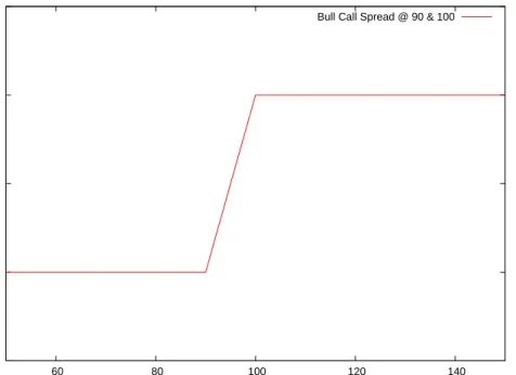
In the paper, the authors provide an example that illustrates this point: we consider two options on the same underlying. We take European call options with the same maturity but different strike prices so as to generate a bull call spread, that is, buying the option with lower strike and selling the option with higher strike. The payoff diagram of this strategy is given in figure 3.1. -5 0 5 10 15 60 80 100 120 140

Bull Call Spread @ 90 & 100

Figure 3.1: Bull call spread payoff diagram

The interest of this strategy is to profit from upward markets. Here, the assumption made is that markets will not go above a certain threshold and so part of the upward potential of the call option strategy would be useless and expensive. Instead of paying for it, we rather sell it by selling another call option. Hence, we only benefit from the upward move until the strike of the sold option is reached. The advantage is that we obtain money by selling an asset that is not valuable in our views of the market. Let us consider for the example the strikes to be atK1=90 andK2=100. This means that we would be expecting

(36)

3.3 The uncertain volatility model 29

Now, we turn to the valuation of this option portfolio. The first thing to do is to determine the dynamics of the underlying. Here, we will assume it to follow a Black Scholes process with a risk free rate of 5%. Moreover, we assume the volatility to be comprised between

σmi n=10% andσmax=40%. With these assumption for the dynamics of the underlying

we provide in the following several valuations of this bull call spread.

The first possible approach is to take a best/worst case analysis. By doing so, we value the option that we are buying with the highest volatility (which gives the highest price) and the option that we sell with the lowest volatility. However, we clearly see that this approach is not consistent, since we would be using different volatilities to price options on the same underlying at the same point in time. This could only make sense if we considered a strike-dependent volatility (see volatility smile theories).

The new approach proposed in the paper consists in valuing the portfolio as a whole. Us-ing the methodology suggested by the authors, we roll-back the final scenarios accordUs-ing to the measures defined by the underlying processes taking at each step the volatility that values the portfolio at its worst. This approach, as previously discussed, will give tighter bounds for the bid and ask prices that will hedge the volatility risk away.

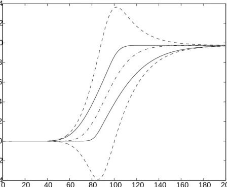
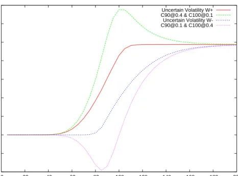
Finally, the authors also provide as benchmark the portfolio evaluated by standard Black Scholes method using one single volatility: the midpoint of the interval. The results ob-tained by this approach are presented in figure 3.2

The thick lines correspond to the upper and lower bounds provided by the proposed method. The outer dotted lines are the prices obtained using a best/worst case approach with the Black Scholes formula and the middle line is a Black Scholes price with mid volatility. Here we observe the anticipated features: the price range that is needed to inte-grate volatility risk in the model is tighter that a simple best/worst case analysis.

Let us turn now to the applications of the model. In the previous chapter we talked about model risk; the uncertain volatility model helps to quantify and deal with the risk related to the specification of volatility.

First, and straightforward, the quantification of the risk comes from the bid-ask quotes produced by the model. These quotes give information on extreme scenarios contrary to the original Black Scholes model which produces a simple quote with no reference what-soever to its variability to volatility changes -the only measure is the artificial vega, theo-retically inconsistent and misleading in practice.

(37)

0 20 40 60 80 100 120 140 160 180 200 −4 −2 0 2 4 6 8 10 12 14

Figure 3.2: Bull call spread valuation

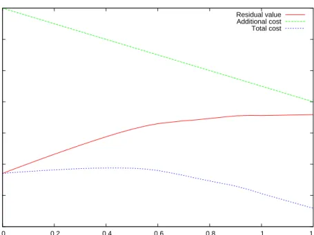
The second application is somehow a consequence of the quantification of the risk. The Lagrangian Uncertain Volatility model [APEK+_{96] will allow us to decide whether to}

stat-ically hedge a position with other traded instruments. The rationale of such hedging is to fully eliminate the volatility risk as the payoffs of the hedging instruments offset those of the liabilities. However, often static hedging is expensive and in a classical framework it is difficult to decide if it is worthy. The Lagrangian Uncertain Volatility model uses the quantification of the risk made by the Uncertain Volatility Model to determine the optimal hedging policy.

We illustrate this application in the following with an example. Let us consider, for in-stance, a financial institution that has to quote a price for a given instrument. Whenever the quoted price is accepted by the counterparty, the financial institution will acquire an obligation or liability. If we consider the financial institution to be dealing with several clients, in the end, this will result in a residual liability which is the sum of all the liabilities generated by the contracts.

(38)

3.3 The uncertain volatility model 31

on other liquidly traded instruments whose prices are exogenously given by the market and keeping these positions to maturity so as to offset the liabilities generated by the other operations. This comes at a cost, the cost of taking the positions on the hedging instru-ments. Whenever the hedging instruments are cheaper than the hedged liability, there is a (pseudo)-arbitrage opportunity. The key difference here with respect to Black Scholes classic arguments is that considering different volatility scenarios may alter the prices and, in some cases, the volatility risk transfer will be enough to justify a transaction.

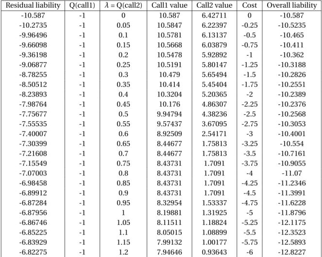
We conclude this section with an example to illustrate the Lagrangian Uncertain Volatility. Consider a bank that has sold a European option. The bank has then a liability corre-sponding to this sold call. When evaluating this liability in the uncertain volatility frame-work, we would take the highest volatility as it is the one that corresponds to the worst scenario. Now, we consider that there is another call trading at an implied volatility higher than our worst case volatility. If the bank buys this second call, it will (statically) hedge a big part of the residual liability. The value of the residual liability will thus be diminished. The lagrangian uncertain volatility model will indicate the optimal quantity of hedging instruments to acquire or short taking into account a given price for the hedging instru-ments and a residual liability.

(39)

(40)

Chapter 4

QuantLib: an introduction

4.1 Aim and scope of the project

Finance is essentially an applied field where having solid theories about prices is essential but where the implementation of such theories is also of vital importance. In the context of constantly changing markets, quoting prices and detecting mispricings must take place fast and accurately. Errors may result in important losses while delays may imply losing clients. The words for this field are therefore fast and reliable.

In this section we focus on the implementation of financial models.

The majority of industry participants believe the implementations to be a competitive advantage factor. Accordingly, they use proprietary software, own-developed or trough closely watched externalization. This translates in an important amount of redundancy in the tasks as algorithms are implemented again and again and often not in the most efficient ways.

Here is where open source can play a relevant role in the years to come.

The idea is to build a common base, available to all practitioners, academics, students, regulatory bodies, and build upon this base. In this way, the standard implementations can be improved and best practices made available to everyone, thus favoring market ef-ficiency which should be the final objective of all the players.

It has to be said that finance is basically about predicting the future and that it makes no 33

(41)

sense to standardize predictions. What is aimed for instead is to standardize the ways to translate, through a given model, a prediction into a price or into any other market mea-sure. The fact of having one efficient implementation of Black Scholes does by no way mean that all banks will use the same input parameters. Ultimately, each financial insti-tution will have to chose what models to use and what parameters to input in the model. By offering standards in implementations of widely used models, one allows the industry participants to focus on what should be their main task. Besides, keeping the solution open-source allows anyone to develop extensions suited to particular needs. Finally, it is easier to build regulations on standards.

It is with this whole perspective that a number of projects have been developed. The one that has gone further down the track is QuantLib.

According to the objectives stated in the project’s website,

The QuantLib project is aimed at providing comprehensive software frame-work for quantitative finance. QuantLib is a free/open-source library for mod-elling trading and risk management in real-life.

The scope of the project is restricted to the implementation of the most used financial models, leaving aside the obtention of market data, whose availability is another issue currently under discussion, especially as open-source gains presence in the financial com-munity.

The project is maintained and developed by a community of programmers. There is a di-vision between authors and contributors, the first being responsible for most of the design and releases while the latter basically submit code or comments according to some spec-ifications. Contributors may also participate in the design through forums in which the authors regularly post and reply. A few companies have devoted significant resources to the development of this library, notably StatPro, a leading international risk-management provider, where the QuantLib project was born.

The QuantLib license is a modified BSD (Berkeley Software Distribution) suitable for use in both free software and proprietary applications, imposing no constraints at all on the use of the library.

(42)

4.2 Organization: an overview 35

4.2 Organization: an overview

In this section we provide an overview of the library structure and organization along with some quick guidelines to develop applications on top of it.

As of January 2009, QuantLib is in its 0.9.7 version and has practically no documenta-tion. This makes it very hard for newcomers to understand how the project is built and it may discourage many from using this solution. The code comments compilated in a pseudo-documentation support are useless to obtain a general view of the structure of the library. However, efforts are being made to put remedy to this issue: one of the devel-opers is writing a book that explains the main design choices and gives a broader view on the library’s structure. However, this documentation is still incomplete and the following section aims at providing the reader with a general understanding of QuantLib from an "undocumented" approach.

QuantLib is written in C++, an object oriented programming language. In Appendix A we provide a short review of the main concepts of object oriented programming while in this section we focus on how they are put together to structure the library.

4.2.1 From the main requirements to the basic class structure

The main objective of QuantLib is to provide means to price financial instruments. The two main requirements for the library are that it should be able to:

• support extensions of the type of instruments priced; • support extensions of the means of pricing the instruments.

These two requirements naturally translate into classes: Instrument and Pricing Engine. These two classes are abstract classes that should be kept as general as possible and only include the attributes and methods shared by all financial instruments and pricing algo-rithms respectively.

This double class structure is interesting as it permits to separate the objectivable descrip-tion of the instrument from the subjective pricing features such as possible dynamics or probability distributions.

(43)

Through inheritance we can account for the complexity of the multiple financial instru-ments and pricing engines while preserving some common interfacing features that will be interesting to design neatly some applications.

The basic structure built from these premises can schematized as follows:

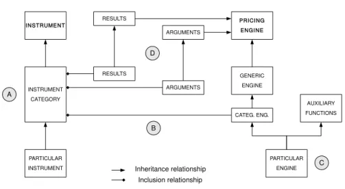
INSTRUMENT INSTRUMENT CATEGORY PRICING ENGINE PARTICULAR INSTRUMENT RESULTS ARGUMENTS RESULTS ARGUMENTS GENERIC ENGINE CATEG. ENG. AUXILIARY FUNCTIONS PARTICULAR ENGINE A B D C Inheritance relationship Inclusion relationship

Figure 4.1: QuantLib structure diagram.

(A) Specific instruments are defined as inheriting from the basic instrument class, often with multiple layers representing wider instrument categories;

(B) Pricing engines will only make sense for some given instrument categories. A gory Engine, inheriting from Pricing Engine is embedded in each Instrument Cate-gory class;

(C) To facilitate the reuse of code, sometimes the pricing functions are coded in a sepa-rate class and the role of the actual pricing engine will be to combine these auxiliary functions into a pricing algorithm;

(D) Parameter passing: each engine will take two templates (arguments and results) that will specify the format of the interactions with the instrument. The classes that will

(44)

4.2 Organization: an overview 37

be passed as templates are thus be embedded in the instrument description while inheriting from the base pricing engine to acquire interaction functionalities.