P
ARIS
-J
OURDAN
S
CIENCES
E
CONOMIQUES
48, BD JOURDAN – E.N.S. – 75014 PARIS
TEL. : 33(0) 1 43 13 63 00 – FAX : 33 (0) 1 43 13 63 10
www.pse.ens.fr
WORKING PAPER N° 2005 - 23
International Equity Holdings and Stock Returns Correlations:
Does Diversification Matter At All for Porfolio Choice?
Nicolas Coeurdacier
Stéphane Guibaud
Codes JEL : G11, G15
Mots clés : International Portfolio Choice, International
Stock Return Correlations, Financial Integration,
Endogeneity Bias
July 2005
International Equity Holdings and Stock Returns Correlations:
Does Diversi
fi
cation Matter At All for Portfolio Choice?
Nicolas Coeurdacier ∗ Stéphane Guibaud† ‡
Abstract
Do investors completely ignore the basics of portfolio theory? Given their over-exposure on domestic risk, investors should try to hedge this risk by picking foreign assets that have low correlation with their home assets. In the data though, we find a robust positive relationship between bilateral equity holdings and bilateral return correlations. We argue that this finding could be driven by the common impact of “financial integration” on cross-border equity holdings and on cross-market correlations. Indeed, when we instrument current correlation with past correlation to control for endogeneity, we recover asset demand functions that decrease with return correlation.
Keywords : International Portfolio Choice, International Stock Return Correlations, Financial Inte-gration, Endogeneity Bias
JEL Codes : G11, G15
∗Paris-Jourdan Sciences Economiques, 48 boulevard Jourdan, 75014 Paris. E-mail: coeurdacier@pse.ens.fr
†Paris-Jourdan Sciences Economiques, 48 boulevard Jourdan, 75014 Paris. E-mail: stephane.guibaud@ens.fr ‡We are grateful to Daniel Cohen, Bernard Dumas, Jean Imbs, Philippe Martin and Richard Portes for useful
discussions and for comments on earlier drafts of this paper. We are also indebted to the participants at the Federation Paris-Jourdan Lunch seminar and at the ADRES seminar, especially to Hubert Kempf for his comments and suggestions.
1
Introduction
Is there any diversification logic driving international portfolio choice? French and Poterba [1991], documenting the existence of a “home bias in portfolio”, clearly pointed at a failure of this logic: due to the variance-covariance structure of home and foreign returns, investors would typically benefit from holding more assets abroad. But one can ask further: is the part of investors portfolios held abroad properly diversified? In particular, given that, for any reason that be, investors are over-exposed on their domestic assets (the home bias in portfolio), they should want to tilt their international holdings towards countries that provide a good hedge for their domestic risk, i.e. countries whose stock market indices have little correlation with their home stock index. Do they? The goal of this paper is to address this question, focusing on aggregate equity holdings.
Recently, following Portes and Rey [2005], a couple of papers in international finance have looked at the determinants of international assetflows and holdings (Aviat and Coeurdacier [2004], Lane and Milesi-Feretti [2004]). These papers typically adopt a methodology imported from the empirical trade literature and run regressions of the following form:
log(assetij) =α+βlogmi+γlogmj+δZij+εij (1)
where assetij is the amount of assets held by country i in country j, mi and mj proxy for the market size of each country andZij is a set of variables affecting bilateral asset holdings. Though such “gravity” equations are not strongly grounded in theory (except for the notable exception of Martin and Rey [2004]), they have proved to perform very well empirically: the elasticity of bilateral asset holdings to the market size of both source and target country is close to one, and variables capturing transaction costs and information asymetries have a significant negative impact.
Throughout the paper, we adopt this gravity equation framework and focus on the impact of bilateral stock return correlations on bilateral equity holdings. Theory tells us that we should
expect a negative relationship. Running a naive regression without controlling for geography and trade, wefind apositive impact of bilateral stock returns correlations on bilateral equity holdings. We confidently interpret this result as spurious, capturing the common impact of geography and trade on equity holdings and on return correlations. Indeed: a) Frankel and Rose [1998] and Imbs [1999] show that trading partners have more correlated business cycles (and Walti [2004] shows they also have more correlated stock returns) while Flavin et al. [2001] show that closer countries have more stock markets comovements; and b) the fact that countries foreign holdings are biased towards geographically close economies and trading partners is the main conclusion of Portes and Rey [2005], Aviat and Coeurdacier [2004] and Lane and Milesi-Feretti [2004]. But this is not the end of the story: when we control for trade and distance, foreign portfolio holdings still appear to be biased towards countries whose assets are the closest substitutes to the domestic ones1 .
Does the positive correlation found in the data at this stage implies rejection of the traditional model of rational portfolio choice? We argue that before to jump to that conclusion, one should make sure that the degree of “financial integration” has been properly controlled for. In our words, the degree of financial integration between countriesi and j refers to the relative easiness with which an investor from countryican invest in country j. This depends on many factors — infor-mational asymetries, transaction costs,fiscal hindrances, familiarity, etc... Saying that (bilateral) foreign investment is positively affected by (bilateral)financial integration is stating the obvious. But returns correlation is also endogenous: for a given correlation of the economic fundamentals, returns correlation increases with the degree of integration. This is because prices comovements are partly induced by portfolio rebalancing between markets (Coeurdacier and Guibaud [2004] make this point in a dynamic equilibrium model). In the context of our empirical investigation, this means that the positive sign reported for the correlation coefficient could result from a pos-itive bias on the OLS estimator due to the endogeneity of the observed level of stock market
1 It is true though that, when we control for these variables, the positive impact of stock market correlation is very much reduced.
correlations.
In order to overcome the suspected endogeneity bias, we had to find an appropriate instru-mentation scheme. Our strategy consists in taking bilateral stock market correlations over the period 1950-1975 to instrument current stock return correlations. We argue that this constitutes a good instrument since until the mid 1970’s most stock markets were segmented (Obstfeld and Taylor [2000], Kaminsky and Schmuckler [2003]), so that the observed correlation over this period, reflecting only the fundamental correlation, is related to current correlation but not to the current degree of financial integration between countries. Indeed, when we run instrumented regression, we recover asset demand functions that decrease with the correlation. Ceteris paribus (i.e. con-trolling for all the obstacles to cross-border investment), a high correlation with the domestic stock market deters investment.
Hence, the message of this paper is that the basic principles of portfolio theory are not com-pletely ignored. This bottom line stands in contrast to a strand of the literature that has come to conclude, as Huberman [2001] puts it, that “People invest in the familiar while often ignoring the principles of portfolio theory”. Though a behavioral approach to investment practices is certainly relevant, traditional portfolio theory should not be completely discarded as a positive theory.
For the remaining of the paper, our roadmap is the following. In section 2, we sketch a model of international portfolio choice featuring home bias in portfolios (taking it as given). We make it clear that, in a world without frictions generating “home bias”, there would be no systematic relationship between cross-border holdings and returns correlation. However, we show that as soon as we assume some home bias in portfolios, an increase in the correlation between country
j assets and domestic assets reduces holdings of country j assets by domestic investors. To test this theoretical prediction, we adopt the same “gravity equation” framework as in Portes and Rey [2005], Aviat and Coeurdacier [2004] and Lane and Milesi-Feretti [2004], using data on bilateral equity holdings. In section 3, we document the “correlation puzzle” and we confirm some
previous results on the geographical determinants of portfolio allocation. In section 4, we tackle the endogeneity issue and show that the “correlation puzzle” vanishes when we instrument present correlation with past correlation. Section 5 concludes.
2
A simple problem of portfolio choice
In this section, we solve the portfolio choice problem of an international investor whose equity portfolio is biased towards domestic assets for exogenous reasons (regulations, transaction or information costs on foreign investment, existence of non-tradable goods...). We show that, under this realistic “home-bias assumption”, assets that are highly correlated with the domestic asset are less attractive. The logic of this result is that, being over-exposed on their domestic risk, investors want to hedge this risk by holding assets that have low correlation with their domestic asset.
2.1
Assumptions
The world is composed ofN+ 1countries. We consider the portfolio choice problem of a “mean-variance” representative investor of country H (the problem is symmetric for investors of other countries) endowed with wealthWH and facing the following menu of assets :
• A risk-free asset with constant returnr.
• N foreign assets (to be understood as risky constant return production technologies). We note Rj the excess expected return of asset j, 1≤j ≤N, over the risk-free rate,RF the
N-dimensional vector of excess expected returns, andΩF the variance-covariance matrix of
those assets.
• A home asset with excess expected returnRHand varianceσ2H. We noteωjthe covariance of the home asset with the foreign assetjandωthe covariance vector (andωT its transposed).
We noteΩthe variance-covariance matrix of the whole set of (home and foreign) risky assets : Ω= σ2 H ωT ω ΩF (2)
We will noteαH the share of wealth invested in the home asset,αj the share invested in the foreign assetj andαFthe N-by-1 vector ofαj’s. The share of wealth invested in the riskless asset is equal to1−αH−PNj=1αj.
Home-bias assumption:we need to introduce some home-bias in this standard static model. To do so, we use a short-cut and assume that the share of wealth invested in domestic assets has to be above a certain level2 α
H. We assume that this constraint will be binding3 , so that:
αH=αH. (3)
2.2
Benchmark case: asset allocations without frictions
To start with, we consider the case without frictions on international capital markets. The un-constrained optimization problem of countryH investor is
max {αH,αF} αHRH+αTFRF+r 1−αH− N X j=1 αj −γ 2 µ αH αTF ¶ Ω αH αF (4)
where γis the coefficient of risk aversion. The portfolio shares solution of this problem are given
by α0H α0F = 1 γΩ −1 RH RF (5)
where the superscript 0 denotes the absence of frictions.
2In some countries there is indeed a maximum authorized threshold for the share of wealth invested in foreign securities.
3 In the symmetric case where all assets have the same risk-return profile and are uncorrelated, it is sufficient thatαH>N1+1, which seems a reasonable assumption.
Absent frictions, there is no heterogeneity among investors and they all hold the same portfolio. Then, introducingα0
ij the share of countryiinvestor’s wealth invested in countryj,m0jthe overall “market capitalization” of country j andW the aggregate wealth of the world, we can trivially write: ∀i,α0ij = m0 j W (6) If we introducee0
ij =α0ijWi the total amount invested by agentiin country j, we get:
log(e0ij) = log(Wi) + log(m0j)−log(W) (7)
This equation can be seen as a “benchmark gravity equation” where the mass termslog(Wi)and
log(m0
j) fully explain the bilateral asset holdings (to a constant): asset holdings of country i in countryj are fully determined by the wealth of agentiand the size of marketj.
2.3
Asset allocations with frictions generating home bias
We now tackle the case where portfolios are biased towards domestic assets for exogenous reasons, with αH = αH. In this case, the portfolio choice problem amounts to the following quadratic maximization problem : max αF αTFRF− γ 2 £ 2αHαTFω+αTFΩFαF ¤ (8)
From thefirst-order conditions, the optimal choice of foreign equities is given by
αF=Ω−F1 · 1 γRF−αHω ¸ (9)
The “home bias assumption” induces a hedging motive in foreign assets demand, which shows up in the second term (inω). As stated in proposition 1 below, when portfolios are biased towards domestic securities, foreign assets that are close substitutes to the domestic ones are less attractive.
Proposition 1: ∀ΩF∈RN∗N,
∂αj
∂ωj
=−¡Ω−F1¢jjαH <0 (10)
with¡Ω−F1¢jjthejthcoefficient on the diagonal of the inverse ofΩ
F.
Proof : as a variance-covariance matrixΩFis symmetric positive. ThenΩ−F1is also symmetric
positive, which implies: ¡Ω−F1¢ jj >0
4 .
The following proposition further characterizes the outcome of the case with frictions, putting emphasis on the way it deviates from the benchmark case without frictions. The constrained foreign portfolio shares are written as the sum of two terms: the world market portfolio shares in the frictionless caseα0
F, and a “hedging component” due to the home bias.
Proposition 2: Constrained foreign equity holdings are :
αF=α0F−(αH−α0H)Ω−F1ω=α
0
F−∆HF (11)
where α0F is the equilibrium vector of foreign portfolio share in absence of home bias and ∆HF ≡(αH−α0H)Ω−
1
F ω.
Proof : in the appendix.
Proposition 2 will help us making sense of the empirical framework that we use in the next section.
3
The “correlation puzzle”
3.1
Empirical methodology
In what follows, we use gravity equations to model bilateral cross-border asset holdings. Portes and Rey [2005], Aviat and Coeurdacier [2004] and Lane and Milesi-Feretti [2004] have shown
4 Notice that proposition 1 also holds in terms of the correlation of asset j with the domestic asset (ρ
j): ∂αj/∂ρj<0.
that bilateral asset holdings are well explained by market sizes,financial market development and variables that proxy for informational and transaction costs between countries (where geographical distance and bilateral trade play a major role). We propose to estimate the following equation :
log(eij) =α+βlog(mimj) +γρij+δZij+εij (12)
where eij represents equity stocks of country j held by investors of country i, mi is the stock market capitalization of countryi, ρij is the correlation of stock returns expressed in US dollars (USD) andZijis a set of control variables (including trade and distance) that might affect bilateral equity holdings between the two markets.
Our theoretical detour in section 2 can shed light on our regression specification5 . From (6) and (11), we can write αij the share of wealth of countryiinvested in countryj as follows:
αij = m0 j W −∆ij= m0 j W (1−δij) (13)
where δij captures the deviation from the frictionless world market portfolio and is increasing in
ρij the correlation between countryi and countryj assets. Given that αij =eij/Wi, we get the following “gravity equation” for international asset holdings, which extends (7) :
log(eij) =λ+ log(Wi) + log(m0j) + log(1−δij) (14)
It can be seen that our specification (12) is not rigorously the counterpart of (14): we use the stock market capitalization of country i as a proxy for its wealth Wi, and we use the observed market capitalization instead ofm0
j(the market capitalization in the hypothetical frictionless case) since the latter is unobservable. Nonetheless, the theoretical insight contained in (14) leads us to expect β to be close to one and γ to be negative, capturing the hedging motive induced by the existence of impediments to investing abroad. As we saw, the latter prediction depends crucially on the fact that markets are imperfectly integrated.
5 For another theoretical foundation of gravity equations for international trade in assets, see Martin and Rey [2000].
3.2
Data presentation
Our dataset is for the year 2001 and our sample contains 28 “source” countries and 41 “destination” countries6 (the country list as well as further details on data sources are in the appendix). Data on cross-border equity holdings (in USD) come from the Coordinated Portfolio Investment Survey provided by the IMF7 . To proxy for market sizes (the mass termlog(m
imj)in (12)), we use the log of the product of “source” and “destination” countries market capitalizations (MarketCapij). To control forfinancial development of both “source” and “destination” countries, we use the log of the product of GDP per capita (GDP-CAPij). For each country, we construct monthly stock market series in US $ from the main stock index for the period 1990-2001. For each country pairs, we compute the stock returns correlation over this period (Correlationij) and for each destination country, we take the average stock return (Returnj) as a proxy for expected return8 .
We add a set of control variables, whose role as key determinants of bilateral asset holdings has been established in previous studies9 . We consider two geographical control variables : dist
ij is the distance (in log) between the two main cities and Borderij is a dummy variable for a common border between country i and j10 . To control for bilateral trade flows, we use data from the
CHELEM database (CEPII, Paris) for the year 2001. Tradeij is the log of imports plus exports between country j and countryi divided by the product of countries GDP, reflecting trade rela-tionships between countries that are not induced by countries sizes11 . We add a dummy variable
for currency unions (CurrencyUnionij) as these probably foster trade in assets by eliminating
6We restricted our sample according to missing values and data availability for historical stock index series. 7 The CPIS reports some zero for very small amounts. We report 0.01 million USD instead of zero except in the Tobit regression.
8We compute the averaged annual return over the period 1990-2000. We drop the period August 1997 - August 1998 for Asian countries as realized stock returns in this crisis period would probably give a poor idea of expected returns in this area.
9Our estimates for the impact of these variables are consistent with previous studies.
1 0 Wefirst added a “Time Difference” variable to control for differences in working hours on stock markets but we dropped it because it did not modify any of the results and did not show up robustly.
1 1We also tried other measures of trade intensity as the one proposed by Frankel (logE x pij+Im pij
GDPi+GDPj)or directed
trade using only imports or exports but it did not affect our results.
exchange rate uncertainty. To take into account the informational determinants of portfolio allo-cation, we use a “Common Language” dummy (Languageij) if countryiand countryj share the same language and a “Colonial Link” dummy (ColonialLinkij) if country j is a former colony of countryior vice versa.
To control forfiscal and legal determinants of transaction costs infinancial markets, wefirst use a dummy for the proximity of legal systems from La Porta et al. [1997, 1998]. We distinguish be-tween “common law” systems (or “English law”), “French law”, “German law” and “Swedish law”. The dummy variable LegalSystemij equals one when source and destination countries have the same legal system. Legal system similarities might reduce information asymmetries and contract-ing costs. We also use bilateral tax treaties to describe the taxation of foreign capital. Although most of the countries we study have a residence-based tax system, they charge withholding taxes when foreigners repatriate dividends, capital gains or interests. To limit double—taxation, several bilateral tax treaties regulate those withholding taxes. FiscalTreatyij is equal to one when such a treaty exists. Finally, to control for unobservable regional variables that might affect bilateral equity holdings, we add some regional dummies in the “destination country” dimension. We have
five such dummies: Europe, North America, Central and South America, Africa, and Asia and Oceania.
3.3
Estimation
Table (1) below presents our regression results. Two main results stand out: βis found to be close to one as expected, but contrary to what theory predicts, γ is found robustly positive — which constitutes a “correlation puzzle”.
When we do not include any control variable in the “gravity equation” (regression (1)), we
find that investors have equity portfolios that are very strongly biased towards countries whose stock market indices are most correlated with their own stock index, completely at odds with the
diversification logic that should drive portfolio choice. However, this regression might be largely biased because of omitted variables that affect simultaneously bilateral equity holdings and the correlation of returns: the “correlation puzzle” might just be the result of a misspecification and
finding the right control variable could be a way to get rid of the puzzle. Trade, geogaphy and
financial development are candidate control variables. Indeed, Flavin et al. [2001] and Walti [2004] respectively find that distance and bilateral trade are important determinants of stock market comovements: stock market synchronization is higher between trading partners and lower between distant economies. And it is also natural to think that deeper markets (developed economies) show higher stock market comovements. At the same time, we know that equity stocks are biased towards trading partners, close economies and deep markets. In regressions (2) and (3), we control for these variables: though the puzzle has been very much reduced (the point estimate of the correlation coefficient has been divided by three) it remains with a very high level of significance. It should be noted that almost all additional variables are significant with the expected sign, which shows the robustness of previous empirical works on the determinants of bilateral asset holdings. These results are not affected in regression (4), where we control for source country fixed-effect (FE) by estimating the following regression:
log(eij) =αi+βlog(mj) +γρij+δZij+εij (15)
This specification allows us to control for discrepancies between source-country wealth (the rel-evant variable in theory) and market capitalization (the proxy we use). In regression (5), we run a Tobit regression, as our variable Equityij is left-censored with some zeros in the series. In regression (6), we look at the sub-sample of rich countries. The “correlation puzzle” remains.
Equityij (1) (2) (3) (4) (5) (6) MarketCapij 0.88 ∗∗∗ (0.04) 1.03∗∗∗ (0.04) 1.04∗∗∗ (0.04) 1.26∗∗∗ (0.05) 1.06∗∗∗ (0.04) 0.99∗∗∗ (0.04) Correlationij 7.36 ∗∗∗ (0.54) 3.29∗∗∗ (0.56) 2.86∗∗∗ (0.57) 1.72∗∗∗ (0.55) 2.95∗∗∗ (0.59) 2.57∗∗∗ (0.57) Returnj 3.09 ∗∗ (1.60) 0.01 (1.37) − 0.16 (1.36) − 0.39 (1.20) − 0.79 (1.41) 2.60∗∗ (1.33) GDP_CAPij 0.61 ∗∗∗ (0.07) 0.62∗∗∗ (0.07) 0.10 (0.08) 0.64∗∗ (0.07) 1.06∗∗∗ (0.15) distij −0.61 ∗∗∗ (0.10) − 0.49∗∗∗ (0.11) − 0.14 (0.12) − 0.45∗∗∗ (0.11) − 0.11 (0.10) Borderij −(00.33).09 − 0.15 (0.34) 0.23 (0.31) − 0.16 (0.35) − 0.10 (0.28) Tradeij 0.22 ∗∗∗ (0.08) 0.20∗∗∗ (0.08) 0.53∗∗∗ (0.09) 0.24∗∗∗ (0.08) 0.24∗∗∗ (0.08) CurrencyUnionij 0.62 ∗∗∗ (0.23) 0.55∗∗∗ (0.21) 0.64∗∗∗ (0.23) 0.94∗∗∗ (0.18) LegalSystemij 0.27 ∗ (0.16) 0.26∗ (0.15) 0.29∗ (0.17) 0.13 (0.16) Languageij (00..1817) (00..0718) (00..1418) 0.51 ∗∗∗ (0.16) ColonialLinkij (00..3332) (00..30)24 (00..3633) (00..0734) FiscalTreatyij 0.30 ∗∗ (0.15) 0.08 (0.14) 0.31∗∗ (0.15) − 0.08 (0.14)
Estimation OLS OLS OLS FE Tobit OLS
R2 0.61 0.74 0.75 0.74 / 0.76
Number of Obs. 945 880 880 880 880 516
Table 1 : The Correlation Puzzle(Gravity Model for Equity Holdings)
Standard errors are in parenthesis. Statistical significance at the 1% level (resp. 5% and 10%) is denoted by∗∗∗(resp. ∗∗ and∗).
Regression (6) is run on the sub-sample of rich countries (GDP per capita>10 000$). Regional dummies are always included but estimates are not reported.
4
Solving the puzzle : instrumental variable estimates
4.1
An omitted variable bias
Are investors completely numb? Is it really the case that ceteris paribus they would choose to invest in priority in foreign assets highly correlated with the main source of risk they are exposed to? We argue that the puzzling positive relationship documented in the previous section could be driven by the fact that the influence of the degree of market integration has not been entirely neutralized by our control variables. By degree offinancial integration, we mean the size of obstacles to foreign equity holdings — regulations, informational asymetries, transaction costs, fiscal hindrances, or other impediments, some of which are unobservable. If deeper integration leads simultaneously to higher levels of cross-border equity holdings and to higher return comovements, the positive sign ofγ could just come from an omitted variable bias.
Returns correlations are endogenous indeed. The correlation effect we have in mind appears naturally in asset pricing models where returns dynamics are fully endogenized (see Dumas, Harvey and Ruiz [2003], Cochrane et al. [2003], Bhamra [2002], Coeurdacier and Guibaud [2004]). In these models, bilateral stock returns correlations are equilibrium outcomes that are affected by the degree offinancial markets integration. The theoretical prediction is that asfinancial markets integration rises, asset returns between countries are getting more synchronous. The intuition of the mechanism that leads a higher level of integration to induce a higher level of stock return correlations (for a given level of correlation of the "fundamentals") is easy to catch. Take the case of two countries and two assets, one in each country, with imperfectly correlated dividends and consider the impact on asset prices of a good shock on domestic dividends. If both markets are completely segmented, this good shock on the domestic asset will drive its price up without affecting the foreign asset price. Now, if both markets are perfectly integrated, the increase in the domestic asset price will lead the investor to rebalance part of her portfolio towards the foreign asset — because her exposure to domestic risk has increased with the increase in the
domestic asset price. The required rate of return on the foreign asset decreases (because its diversification property are now more cherished) and the foreign asset price must increase to restore equilibrium. This rebalancing effect naturally leads to more comovement between domestic and foreign asset prices than in the fully-segmented world. The impact of the level of financial integration on returns correlations has been established empirically by Bekaert and Harvey [2000]: for a sample of emerging economies, they found that equity market liberalization increases stock markets comovement of countries with the rest of the world. Looking at stock returns correlation between countries over 150 years, Goetzmann and Rouwenhorst [2002] find that the correlation vary considerably through time and is significantly higher during periods offinancial integration.
Because we cannot really capture the degree of integration (to be understood as the size of all obstacles to bilateral equity holdings), we cannot perfectly control for this variable in the regression, which leads our estimate to be biased upward. We show in the appendix that it is possible that this missing variable bias switches the sign of the impact of stock market correlation on equity holdings. To get rid of this endogeneity bias, we need to use an instrumental variable for the stock market correlation.
4.2
Instrumental variables methodology
We propose to instrument the stock market correlation in the nineties by its value over the period 1950-1975. We construct historical correlations in USD (Correlation50-75ij) using monthly stock market data over the period 1950-1975 for our sample of countries. We argue that it provides a good instrument for two reasons. First, a large part of recent correlations is explained by past correlations. This is not surprising as we can expect fundamental comovements to be persistent. The first-stage regression (Correlationij = α+β Correlation50-75ij +εij) performs very well (the T-stat for β is equal to 12.53 and the R-square of the regression is 0.15). Second, the observed correlation before the mid-1970’s reflects much more the fundamentals than nowadays since financial markets were highly segmented in the fifties-sixties (see figure (1) in appendix,
taken from Obstfeld and Taylor [2002]). Stock market liberalization occurred in the eighties for most countries (for precise timing, see Kaminsky and Schmuckler [2003]). Before, cross-border shareholdings were very marginal and international asset trade was mainly borrowing and lending (Kraay and Ventura [2000]). For a sample of OECD countries, Lane and Milesi-Ferreti [2003] show that even at the beginning of the 1980’s, aggregate cross-border equity and FDI assets represented only 10% of aggregate GDP. In 2000, this ratio had jumped to 80%. Our computed historical correlation constitute a “good” instrument as this variable is all at once a powerful predictor of the actual correlation and exogeneous to the degree of market integration.
4.3
Instrumental variable estimation
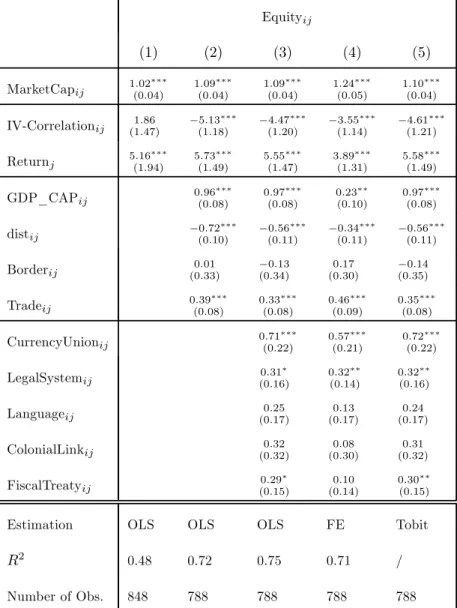
Table (2) shows our estimation results with the instrumented correlation and the same set of control variables as before. The results are remarkable : first, when we do not control for geography and trade, the puzzle does not disappear. Second, once control variables are included, wefind that the correlation has a negative impact on the demand for foreign stocks. This result is robust at reasonable level of significance in all regressions12 . The “correlation puzzle” vanishes: investors
do not behave exactly opposite to the recommendations of portfolio choice theory.
The fact that the estimate of the impact of correlation switches from positive to negative, i.e. the fact that the bias when we do not control for endogeneity is large enough to overturn the sign of the point estimate, is consistent with the fact that theoretical papers have found the positive impact of market integration on return correlation to be rather small (this shows up in the role of coefficientλin the "Omitted variable bias" appendix).
1 2Only the estimate with source countryfixed-effect is not significant at the 1% level (it is significant at a 10% level).
Equityij (1) (2) (3) (4) (5) MarketCapij 1.02 ∗∗∗ (0.04) 1.09∗∗∗ (0.04) 1.09∗∗∗ (0.04) 1.24∗∗∗ (0.05) 1.10∗∗∗ (0.04) IV-Correlationij (11..8647) −5.13 ∗∗∗ (1.18) − 4.47∗∗∗ (1.20) − 3.55∗∗∗ (1.14) − 4.61∗∗∗ (1.21) Returnj 5.16 ∗∗∗ (1.94) 5.73∗∗∗ (1.49) 5.55∗∗∗ (1.47) 3.89∗∗∗ (1.31) 5.58∗∗∗ (1.49) GDP_CAPij 0.96 ∗∗∗ (0.08) 0.97∗∗∗ (0.08) 0.23∗∗ (0.10) 0.97∗∗∗ (0.08) distij −0.72 ∗∗∗ (0.10) − 0.56∗∗∗ (0.11) − 0.34∗∗∗ (0.11) − 0.56∗∗∗ (0.11) Borderij (00..0133) − 0.13 (0.34) 0.17 (0.30) − 0.14 (0.35) Tradeij 0.39 ∗∗∗ (0.08) 0.33∗∗∗ (0.08) 0.46∗∗∗ (0.09) 0.35∗∗∗ (0.08) CurrencyUnionij 0.71 ∗∗∗ (0.22) 0.57∗∗∗ (0.21) 0.72∗∗∗ (0.22) LegalSystemij 0.31 ∗ (0.16) 0.32∗∗ (0.14) 0.32∗∗ (0.16) Languageij (00..2517) (00..1317) (00..2417) ColonialLinkij (00..3232) (00..0830) (00..3132) FiscalTreatyij 0.29 ∗ (0.15) 0.10 (0.14) 0.30∗∗ (0.15)
Estimation OLS OLS OLS FE Tobit
R2 0.48 0.72 0.75 0.71 /
Number of Obs. 848 788 788 788 788
Table 2 : Gravity Model for Equity Holdings using Instrumented Stock Return Correlation
Standard errors are in parenthesis. Statistical significance at the 1% level (resp. 5% and 10%) is denoted by∗∗∗(resp. ∗∗ and∗).
Correlationij is instrumented according to the followingfirst-stage regression :
Correlationij =α+β Correlation50-75ij+εij
β is significant at the 1% level (T-Stat=12.53). First-stage regression is not shown but available on request.
Regional dummies are always included but estimates are not reported.
4.4
Robustness checks
Correlation transformation: it might be argued that due to the fact that correlations take value over the bounded interval [−1,1], error terms are not normally distributed. We checked for this concern by using log((1 +correl)/(1−correl))in our regressions, as suggested in Otto, Voss and Willard [2001]. Our results were not affected.
“Rich” Countries Sample: we checked the robustness of our results by restricting our sample to “rich” countries. Countries in this sub-sample have a GDP per capita higher than 10 000 USD (the cut-off country is Greece). Data for those countries are probably more accurate. All our results are confirmed qualitatively and quantitatively (table 3 below).
Equityij (1) (2) (3) (4) MarketCapij 0.87 ∗∗∗ (0.04) 1.05∗∗∗ (0.04) 1.05∗∗∗ (0.04) 1.17∗∗∗ (0.04) IV-Correlationij (16..0359) −3.90 ∗∗ (1.79) − 3.54∗∗ (1.74) − 4.23∗∗∗ (1.64) Returnj 7.44 ∗∗∗ (1.95) 3.76∗∗∗ (1.26) 3.27∗∗∗ (1.25) 3.86∗∗∗ (1.09) GDP_CAPij 0.77 ∗∗∗ (0.17) 1.07∗∗∗ (0.17) 0.47∗∗∗ (0.19) distij −0.44 ∗∗∗ (0.08) − 0.22∗∗ (0.09) − 0.28∗∗∗ (0.09) Borderij (00..0928) − 0.03 (0.29) 0.09 (0.25) Tradeij 0.45 ∗∗∗ (0.08) 0.44∗∗∗ (0.08) 0.46∗∗∗ (0.08) CurrencyUnionij 0.97 ∗∗∗ (0.18) 1.15∗∗∗ (0.17) LegalSystemij (00..1417) −(00.15).05 Languageij 0.32 ∗∗ (0.16) − 0.06 (0.15) ColonialLinkij (00..0135) (00..1232) FiscalTreatyij (00..0914) (00..0113)
Estimation OLS OLS OLS FE
R2 0.53 0.72 0.74 0.73
Number of Obs. 541 516 516 516
Table 3 : Gravity Model for Equity Holdings using Instrumented Stock Return Correlation (Rich Countries Sample)
Standard errors are in parenthesis. Statistical significance at the 1% level (resp. 5% and 10%) is denoted by∗∗∗(resp. ∗∗ and∗).
Correlationij is instrumented according to the followingfirst-stage regression :
Correlationij =α+β Correlation50-75ij+εij
β is significant at the 1% level . First-stage regression is not shown but available on request. Regional dummies are always included but estimates are not reported.
5
Conclusion
Under realistic assumptions, foreign assets that provide good hedge for domestic risk should be more attractive to domestic investors: if investors hold “home-biased” portfolios, they should tilt their foreign holdings towards assets that have low return correlation with the domestic ones. In this paper, we proposed to test this simple hypothesis in a “gravity equation” setup using aggregate data on bilateral equity holdings.
Running OLS regressions of bilateral correlation of stock returns on bilateral equity holdings we found that asset holdings increase with the correlation of stock returns between countries, at odds with what theory predicts. We then showed that this “puzzle” vanishes when the endogeneity of returns correlation is properly taken into account. The point is that the correlation of asset returns is itself an equilibrium outcome — which is affected by the degree offinancial market integration: an increasing degree of market integration leads to higher comovements of stock returns. Tofind a source of variations in current return correlations that is exogenous to the degree of market integration, we used bilateral stock return correlation over the period 1950-1975: before the mid 1970’s, markets were highly segmented and the observed correlation was purely reflecting the “fundamentals”. This instrumentation scheme allowed us to recover asset demand functions that decrease with returns correlation.
Ourfinding that diversification actually matters for international portfolio choice is somewhat dissonant compared to what people have come to believe. Our work restores some credit for the empirical validity of portfolio choice theory at an international level: even though they can exhibit bounded rationality, over-confidence and a naive approach to diversification, investors are not completely heedless to the basic logic of the textbook mean-variance model of portfolio choice.
Acknowledging that assets returns correlation — i.e. assets “substituability” — is endogenous was crucial in getting ourfinal result. Beyond the context of this paper, we believe more theoretical
and empirical work remains to be done on the determinants of financial markets comovements. Since the early 1970’s, the correlation between US monthly stock returns (S&P500) and a synthetic non-US world index has increased by 0.1 each decade, rising continuously from 0.4 in 1970 to 0.71 in 200013 . To our knowledge, there exists no compelling explanation for this huge rise in stock markets “synchronization”. One such explanation is very much required.
1 3In August 2004, the correlation (computed on a 5-year window) had risen up to 0.82.
6
Appendix
6.1
Proof of proposition 2
In the case without frictions, we have
Ω α0H α0 F = 1 γ RH RF Besides, by definition ofΩ, Ω α0 H α0 F = σ2 H ωT ω ΩF α0 H α0 F = σ2 Hα0H+ωTα0F α0 Hω+ΩFα0F
Then, concentrating on the bottom part of thefirst equation, we get
1 γRF=α 0 Hω+ΩFα0F Substituting for 1 γRFinαF=Ω− 1 F h 1 γRF−αHω i yields: αF = Ω−F1 · 1 γRF−αHω ¸ = α0F−(αH−α0H)Ω−F1ω
6.2
Data sources
• Bilateral Exports and Imports: in 2001, in US Dollars from the CHELEM dataset (Centres d’Etudes Propectives et d’Informations Internationales, CEPII, Paris).
• Bilateral Equity Holdings: in US dollars, in 2001, from the Coordinated Portfolio Invest-ment Survey, http://www.imf.org/external/np/sta/pi/datarsl.htm. When equity holdings are “very small” (the smallest value reported is 10 000$), the dataset reports a zero. We consider those zeros to be equal to 0.01 million USD (except in the Tobit estimation).
• GDP and GDP/capita : from the International Financial Statistics.(GDP in US dollars in 2001, exchange rates used are also from the IFS).
• Geography Variables: in km, from S—J Wei’s website and from various sources (“How far is it ?”, http://www.indo.com/distance )
• Common Language and Colonial Link: various sources (for colonial link, mainly sum-maries of country history in Encyclopedias.)
• Legal Variable: mainly La Portaet al. [1998], various sources for missing countries14 . • Tax Treaty Variable: IBFD online products (http://www.ibfd.org); Latin American
Tax-ation Database, European TaxTax-ation Database, Asia—Pacific Taxation Database, Tax Treaties Database.
• Stock Market Returns: monthly end-of-period data from 1950 to 2001 in Local Currency from Global Financial Data. Converted in USD using end-of period Exchange Rate from the same dataset.
1 4http://www.llrx.com
6.3
Geographical sample
Source Countries
Australia, Austria, Belgium, Canada, Chile, Denmark, Finland, France, Germany, Greece, Hong Kong, Ireland, Italy, Japan, Korea, Luxemburg, Malaysia,
Netherlands, Norway, New Zealand, Portugal, Singapore, South Africa, Spain, Sweden, Switzerland, United Kingdom, United States
Destination Countries
Europe:
Austria, Belgium, Denmark, Finland, France, Germany, Greece, Ireland, Italy, Luxembourg,
Netherlands, Norway, Portugal, Spain, Sweden, Switzerland,United Kingdom
Israel, Turkey Asia & Oceania: Australia, Hong Kong, Indonesia, Japan, Malaysia, New Zealand, Philippines,
Singapore, South Korea, Taiwan, Thailand North America:
Canada, United States Central & South America:
Argentina, Brazil, Chile, Colombia, Mexico, Peru Africa:
Morocco, Nigeria, South Africa
6.4
Descriptive statistics
All variables are expressed in log (except stock market correlations)
Mean Std Min Max N
Equityij 5.00 3.64 -4.605 12.76 945 Tradeij -18.80 1.22 -22.34 -13.46444 1014 MarketCapij 23.90 2.11 18.78 30.85 1080 log(Distanceij) 8.55 1.04 5.25 9.89 1080 Correlationij 0.393 0.187 -0.135 0.875 1080 Correlation50-75ij 0.166 0.155 -0.208 0.961 945 Returnj 0.048 0.062 -0.078 0.215 41 GDP-CAPij 19.01 1.37 13.69 21.03 1080
6.5
Omitted Variable Bias
Let us noteIij the degree of market integration between the two markets. Then we can write the following system of equations:
Equityij = α−γCorrelationij+δIij+ηZij1 +εeij Correlationij = θ+λIij+εcij
where γ, δ, λ are expected to be strictly positive, εe
ij and εcij are uncorrelated and normally distributed with zero mean and respective varianceσ2
eandσ2c, andZij1 is a set of control variables (including market sizes, distance, etc.). For simplicity, we supposeZ1
ij is orthogonal to the other explaining variables.
In section 3, we estimated the following equation
Equityij=α−γˆCorrelationij+ ˆηZij1 +ζij
where ζij is normally distributed with zero mean and varianceσ2ζ. According to the true model, we estimated : Equityij = α−γCorrelationij+δ ·Correlation ij−θ+εcij λ ¸ +ηZij1 +εeij = α−δθ λ − · γ−δ λ ¸ Correlationij+ηZij1 +εeij− δεcij λ Hence: E[ˆγ] =γ− δ λ
Since λδ >0, our estimator is biased — the correlation variable is spuriously catching the effect of market integration on equity holdings. If λδ > γ, a positive relationship between Correlationij and Equityij is to be expected, consistently with our estimations in section 3.
How plausible is the switch in the sign of the correlation variable?
The condition for the bias to be large enough is λδ > γ. This happens if the impact of market integration on equity holdings (characterized byδ) is large relative to the impact of market integration on stock returns correlation (characterized byλ).
In a companion paper (Coeurdacier and Guibaud [2004]), we show that the degree of market integration has a first-order effect on bilateral equity holdings but is affecting stock returns cor-relation only to a second-order. This is consistent with the switch in the sign of the corcor-relation variable that we get in section 4.
Figure 1: A Stylized View of Capital Mobility (Obstfeld and Taylor, [2002])
References
Aviat, A., Coeurdacier, N. , 2004. The Geography of International Trade in Goods and Asset Holdings. Unpublished working paper. Paris-Jourdan Sciences Economiques.
Bekaert, G., Harvey, C.R. , 1995. Time-Varying World Market Integration. Journal of Fi-nance, 50, 403-444.
Bekaert, G., Harvey, C. R., 2000. Foreign speculators and emerging equity markets. Journal of Finance, 55, 564-614.
Bhamra, H.S., 2004. International Stock Market Integration: A Dynamic General Equilib-rium Approach. Unpublished working paper. London Business School.
Chan, K., Covrig, V.M., Ng, L.K., 2005. What Determines the Domestic and Foreign Bias? Evidence from Mutual Fund Equity Allocations Worldwide. Journal of Finance, 60, 1495-1534.
Cochrane, J., Longstaff, F. and Santa Clara, P., 2003. Two Trees: Asset Price Dynamics Induced by Market Clearing. Unpublished working paper. University of Chicago, UCLA. Coeurdacier, N., Guibaud, S., 2004. A Dynamic Equilibrium Model of Imperfectly Integrated Financial Markets. Unpublished working paper. Paris-Jourdan Sciences Economiques. Dumas, B., Harvey, R., Ruiz, P., 2003. Are Correlation of Stock Returns Justified by Sub-sequent Changes in National Outputs?. Journal of International Money and Finance, 22, 777-811.
Flavin, T.J, Hurley, M.J, Rousseau, F., 2001. Explaining Stock Market Correlation: A Gravity Model Approach. The Manchester School, 70, 87-106.
Frankel, J., Rose, A., 1998. The Endogeneity of the Optimum Currency Area Criteria. Economic Journal, Vol. 108, 449, 1009-1025.
Frankel, J., Rose, A.K., 2002. An Estimate of the Effect of Common Currencies on Trade and Income. The Quarterly Journal of Economics, 117 (2), 437—466.
French, K., Poterba, J., 1991. Investor Diversification and International Equity Markets. American Economic Review, 81 (2), 222-26.
Goetzmann, W., Li, L., Rouwenhorst, K., 2002. Long-term global market correlation. Un-published working paper. Yale University.
Guibaud, S., 2004. Endogenous Borrowing Constraints in the Presence of Shipping Costs. Unpublished working paper. Paris-Jourdan Sciences Economiques.
Henry, P., 2000. Stock Market Liberalization, Economic Reform and Emerging Market Eq-uity Prices. Journal of Finance, 55, 529-564.
Huberman, G., 2001. Familiarity Breeds Investment. The Review of Financial Studies, 14 (3), 659-680
Imbs, J., 1999. Trade, Finance, Specialization and Synchronization. Review of Economics and Statistics. 86(3)
Kaminsky, G., Schmukler, S., 2003. Short-Run Pain, Long-Run Gain: The Effects of Finan-cial Liberalisation. IMF Working Paper, 34.
Lane, P., Milesi-Feretti, G.M., 2003. International Financial Integration. IMF StaffPapers, 50.
Lane, P., Milesi-Feretti, G.M., 2004. International Investment Patterns. Unpublished work-ing paper. CEPR Discussion Paper, 4499.
La Porta, R., Lopez-de-Silanes, F., Schleifer, A., Vishny, R.W., 1997. Legal Determinants of External Finance. Journal of Finance, 52, 1131-1150
La Porta, R., Lopez-de-Silanes, F., Schleifer, A., Vishny, R.W., 1998. Law and Finance. Journal of Political Economy, 106, 1113-1155.
La Porta, R., Lopez-de-Silanes, F., Schleifer, A., 2004. What Works in Securities Laws?. Unpublished working paper. Yale University, and Harvard University.
Martin, P. ,Rey, H., 2004. Financial Super-Markets: Size Matters for Asset Trade. Journal of International Economics, 64, 335-361.
Obstfeld, M., 1994. Risk-Taking, Global Diversification and Growth. American Economic Review, 84, 1310-29.
Obstfeld, M., Rogoff, K., 2000. The Six Major Puzzles in International Macroeconomics: Is There a Common Cause?. NBER Macroeconomics Annual.
Obstfeld, M., Taylor, A.M, 2002. Globalization and Capital Markets. Unpublished working paper. NBER Working Paper 8846.
Otto, G., Voss, G., Willard, L., 2001. Understanding OECD Output Correlations. Unpub-lished working paper. Reserve Bank of Australia.
Portes, R., Rey, H., 2005. The Determinants of Cross-Border Equity Flows. Journal of International Economics, 65(2), 269-296.
Portes, R., Oh, Y., Rey, H., 2001. Information and Capital Flows: The Determinants of Transactions in Financial Assets. European Economic Review, 45 (4-6), 783-96.


![Figure 1: A Stylized View of Capital Mobility (Obstfeld and Taylor, [2002])](https://thumb-us.123doks.com/thumbv2/123dok_us/1003032.2632032/29.892.224.684.180.525/figure-stylized-view-capital-mobility-obstfeld-taylor.webp)
