Risk, Uncertainty and Asset Prices

NBER WORKING PAPER SERIES

RISK, UNCERTAINTY AND ASSET PRICES

Geert Bekaert

Eric Engstrom

Yuhang Xing

Working Paper 12248

http://www.nber.org/papers/w12248

NATIONAL BUREAU OF ECONOMIC RESEARCH

1050 Massachusetts Avenue

Cambridge, MA 02138

May 2006

Corresponding author: Columbia Business School, 802 Uris Hall, 3022 Broadway, New York New York, 10027; ph: (212)-854-9156; fx: (212)-662-8474; gb241@columbia.edu. We thank Bob Hodrick, Charlie Himmelberg, Kobi Boudoukh, Tano Santos, Pietro Veronesi, Francisco Gomes and participants at presentations at the Federal Reserve Board and the WFA, Portland 2005 for helpful comments. The views expressed in this article are those of the authors and not necessarily of the Federal Reserve System. The views expressed herein are those of the author(s) and do not necessarily reflect the views of the National Bureau of Economic Research.

©2006 by Geert Bekaert, Eric Engstrom and Yuhang Xing. All rights reserved. Short sections of text, not to exceed two paragraphs, may be quoted without explicit permission provided that full credit, including © notice, is given to the source.

Risk, Uncertainty and Asset Prices

Geert Bekaert, Eric Engstrom and Yuhang Xing

NBER Working Paper No. 12248

May 2006

JEL No. G12, G15, E44

ABSTRACT

We identify the relative importance of changes in the conditional variance of fundamentals (which

we call “uncertainty”) and changes in risk aversion (“risk” for short) in the determination of the term

structure, equity prices and risk premiums. Theoretically, we introduce persistent time-varying

uncertainty about the fundamentals in an external habit model. The model matches the dynamics of

dividend and consumption growth, including their volatility dynamics and many salient asset market

phenomena. While the variation in dividend yields and the equity risk premium is primarily driven

by risk, uncertainty plays a large role in the term structure and is the driver of counter-cyclical

volatility of asset returns.

Geert Bekaert

Columbia Business School

802 Uris Hall

3022 Broadway

New York, NY 10027

and NBER

gb241@columbia.edu

Eric Engstrom

Mail Stop 89

Board of Governors of the Federal Reserve System

Washington, DC 20551

eric.c.engstrom@frb.gov

Yuhang Xing

Jones Graduate School of Management

MS 531

Rice University

6100 Main Street

Houston, TX 77005

yxing@rice.edu

1

Introduction

Without variation in discount rates, it is difficult to explain the behavior of aggregate stock prices within the confines of rational pricing models. An old literature, starting with Pindyck (1988), focused on changes in the variance of fundamentals as a source of pricefluctuations, suggesting that increased variances would depress prices. Poterba and Summers (1986) argued that the persistence of return variances does not suffice to account for the volatility of observed stock returns, whereas Barsky (1989) was thefirst to focus attention on the fact that increased uncertainty may also affect riskless rates in equilibrium which may undermine the expected price effects. Abel (1988) examined the effects of changes in the riskiness of dividends on stock prices and risk premiums in a Lucas (1978) general equilibrium model, with the perhaps surprising result that increased riskiness only lowers asset prices when the coefficient of risk aversion is lower than one.

Changes in the conditional variance of fundamentals (either consumption growth or dividend growth) as a source of asset pricefluctuations are making a comeback in the recent work of Bansal and Yaron (2004), Bansal, Khatchatrian and Yaron (2002), and Bansal and Lundblad (2002), which we discuss in more detail below. Nevertheless, most of the recent literature has not focused on changes in the variability of fundamentals as the main source offluctuations in asset prices and risk premiums but on changes in risk aversion and risk preferences. The main catalyst here was the work of Campbell and Cochrane (1999), CC henceforth, who showed that a model with counter-cyclical risk aversion could account for a large equity premium, substantial variation in returns and price-dividend ratios and long-horizon predictability of returns. There have been a large number of extensions and elaborations of the CC framework (see e.g. Bekaert, Engstrom and Grenadier (2004), Brandt and Wang (2003), Buraschi and Jiltsov (2005), Menzly, Santos and Veronesi (2004), and Wachter (2004)) and a large number of articles trying tofind an economic mechanism for changes in aggregate prices of risk (Chan and Kogan (2002), Lustig and Van Nieuwerburgh (2003), Santos and Veronesi (2000), Piazzesi, Schneider and Tuzel (2003), and Wei (2003)).

In this article, we try to identify the relative importance of changes in the conditional variance of fundamentals (which we call “uncertainty”) and changes in risk aversion (“risk” for short)2. We build 2_{Hence, the term uncertainty is used in a different meaning than in the growing literature on Knightian uncertainty,}

see for instance Epstein and Schneider (2004). It is also consistent with a small literature in internationalfinance which has focused on the effect of changes in uncertainty on exchange rates and currency risk premiums, see Hodrick (1989, 1990) and Bekaert (1996). The Hodrick (1989) paper provided the obvious inspiration for the title to this paper.

on the external habit model formulated in Bekaert, Engstrom and Grenadier (2004) which features stochastic risk aversion and introduce persistent time-varying uncertainty in the fundamentals. We explore the effects of both on price dividend ratios, equity risk premiums, the conditional variability of equity returns and the term structure, both theoretically and empirically. To differentiate time-varying uncertainty from stochastic risk aversion empirically, we use information on higher moments in dividend and consumption growth and the conditional relation between their volatility and a number of instruments.

The model is consistent with the empirical volatility dynamics of dividend and consumption growth and matches a large number of salient asset market features, including a large equity premium and low risk free rate and the volatilities of equity returns, dividend yields and interest rates. We

find that variation in the equity premium is driven by both risk and uncertainty with risk aversion dominating. However, variation in asset prices (consol prices and dividend yields) is primarily due to changes in risk. These results arise because risk aversion acts primarily as a level factor in the term structure while uncertainty affects both the level and the slope of the real term structure and also governs the riskiness of the equity cash flow stream. Consequently, our work provides a new perspective on recent advances in asset pricing modelling. We confirm the importance of economic uncertainty as stressed by Bansal and Yaron (2004) and Kandel and Stambaugh (1990) but show that changes in risk are critical too. However, the main channel through which risk affects asset prices in our model is the term structure, a channel shut offin the original Campbell and Cochrane (1999) paper while stressed by the older partial equilibrium work of Barsky (1989).

The remainder of the article is organized as follows. The second section sets out the theoretical model and motivates the use of our state variables to model time-varying uncertainty of both dividend and consumption growth. In the third section, we derive closed-from solutions for price-dividend ratios and real and nominal bond prices as a function of the state variables and model parameters and examine some comparative statics results. We also demonstrate that two extant models, Abel (1988) and Wu (2001), severely restrict the relationship between uncertainty and equity prices and show why this is so. In the fourth section, we set out our empirical strategy. We use the General Method of Moments (Hansen (1982), GMM henceforth) to estimate the parameters of the model. Thefifth section reports parameter estimates and discusses how well the modelfits salient features of the data. The sixth section reports various variance decompositions and dissects how uncertainty and risk aversion affect asset prices. Section 7 concludes.

2

Theoretical Model

2.1

Fundamentals and Uncertainty

To model fundamentals and uncertainty, we begin with the specification of Abel (1988) but enrich the framework in a number of dimensions. Abel (1988) models log dividends as having a persis-tent conditional mean and persispersis-tent conditional variance and models the stochastic behavior of the conditional mean and the conditional coefficient of variation of dividends. Hence, he assumes that dividends are stationary. We modify this set up to allow for a unit root in the dividend process, as is customary in modern asset pricing, and model dividend growth as having a stochastic volatility process. In addition, we relax the assumption that dividends and consumption are identically equal. While consumption and dividends coincide in the original Lucas (1978) framework and many sub-sequent studies, recent papers have emphasized the importance of recognizing that consumption is

financed by sources of income outside of the aggregate equity dividend stream, for example Santos and Veronesi (2005), and Bansal, Dittmar and Lundblad (2004). Our modeling choice for dividends and stochastic volatility is described by the following equations.

∆dt=µd+ρduut−1+√vt−1 ¡ σddεdt+σdvεvt ¢ (1) vt=µv+ρvvvt−1+σvv√vt−1εvt

where dt = log (Dt) denotes log dividends, ut is the demeaned and detrended log

consumption-dividend ratio (described further below) andvtrepresents “uncertainty,” and is proportional to the

conditional volatility of the dividend growth process. All innovations in the model, including εd t

andεv

t follow independentN(0,1)distributions. Consequently, covariances must be explicitly

para-meterized. With this specification, the conditional mean of dividend growth varies potentially with past values of the consumption-dividend ratio, which is expected to be a slowly moving stationary process. Uncertainty itself follows a square-root process and may be arbitrarily correlated with div-idend growth through theσdvparameter. The sign ofσdvis not a priori obvious. From a corporate finance perspective, an increase in the volatility of firm cash flows may increase the present value of the costs offinancial distress but it may also make growth options more valuable (see Shin and Stulz (2000) for a recent survey). Because it is a latent factor,vtcan be scaled arbitrarily without

We model consumption as stochastically cointegrated with dividends, in a fashion similar to Bansal, Dittmar and Lundblad (2004), so that the consumption dividend ratio, ut, becomes a

relevant state variable. We modelutsymmetrically with dividend growth,

ut=µu+ρu uut−1+σud(∆dt−Et−1[∆dt]) +σuu√vt−1εut. (2)

By definition, consumption growth,∆ct, is

∆ct=δ+∆dt+∆ut = (δ+µu+µd) + (ρdu+ρuu−1)ut−1+ (1 +σud)√vt−1 ¡ σddεdt+σdvεvt ¢ +σuu√vt−1εut. (3)

Note that δ and µu cannot be jointly identified. We proceed by setting the unconditional mean

ofut to zero and then identifyδ as the difference in means of consumption and dividend growth.3

Consequently, the consumption growth specification accommodates arbitrary correlation between dividend and consumption growth, with heteroskedasticity driven by vt. The conditional means

of both consumption and dividend growth depend on the consumption-dividend ratio, which is an AR(1) process. Consequently, the reduced form model for dividend and consumption growth is anARM A(1,1) which can accommodate either the standard nearly uncorrelated processes widely assumed in the literature, or the Bansal and Yaron (2004) specification where consumption and dividend growth have a long-run predictable component. Bansal and Yaron (2004) do not link the long run component to the consumption-dividend ratio as they do not assume consumption and dividends are cointegrated.4

Our specification raises two important questions. First, is there heteroskedasticity in consump-tion and dividend growth data? Second, can this heteroskedasticity be captured using our single latent variable specification? Perhaps surprisingly, there is substantial affirmative evidence regard-ing thefirst question, but to our knowledge none regarding the second question. Ferson and Merrick (1987), Whitelaw (2000) and Bekaert and Liu (2004) all demonstrate that consumption growth volatility varies through time. For our purposes, the analysis in Bansal, Khatchatrian and Yaron (2004) and Kandel and Stambaugh (1990) is most relevant. The former show that price-dividend

3_{The presence ofδmeans thatu}

tshould be interpreted as the demeaned and detrended log consumption-dividend

ratio.

4_{In a recent paper, Bansal, Gallant and Tauchen (2004) show that both a Campbell Cochrane (1999) and a}

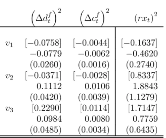
ratios predict consumption growth volatility with a negative sign and that consumption growth volatility is persistent. Kandel and Stambaugh (1990) link consumption growth volatility to three state variables, the dividend yield, the AAA versus T-Bill spread, and the BBB versus AA spread. Theyfind that, consistent with the Bansal et. al. (2004) results, dividend yields positively affect consumption growth volatility. In Table 1, we extend and modify this analysis. We estimate the following model by GMM,

x2_t+k=ν0+ν1rft+ν2dpft +ν3spdt+εt+k (4)

where we alternatively model∆df_t and∆cf_t, (filtered) dividend and consumption growth, asxt.

Be-cause the observable fundamental series arefiltered using a four-period moving average to eliminate seasonality, the prediction lag,k, is set at four quarters. Above,rftis the risk free rate,dpft is the

(also filtered) dividend yield, and spdt is the nominal term spread. We defer a discussion of the

data to Section 4 of the article. Suffice it to say that our analysis uses data starting in 1926 (but we lose one year when calculating lags), whereas the previous papers use post-war samples. We considered an alternative model where time-variation in the conditional means was removed and the conditional variance of the residuals was modelled as in Equation (4). Because consumption and dividend growth display little variation in the conditional mean, the results were quite similar for this case.

The results are reported in Table 1. Panel A focuses on univariate tests while Panel B reports multivariate tests. Wald tests in the multivariate specification very strongly reject the null of no time variation for the volatility of both consumption and dividend growth. Moreover, all three instruments are significant predictors of volatility in their own right: high interest rates are associated with low volatility, high term spreads are associated with high volatility as are high dividend yields. The results in Bansal et al (2004) and Kandel and Stambaugh (1990) regarding the dividend yield predicting economic uncertainty appear robust to the sample period and are also valid for dividend growth volatility.

Note that the coefficients on the instruments for the dividend growth volatility are 5-15 times as high as for the consumption growth equation. This suggests that one latent variable may capture the variation in both. We test this conjecture by estimating a restricted version of the model where the slope coefficients are proportional across the dividend and consumption equations. This restriction

is not rejected, with a p-value of 0.8958. We conclude that our use of a single latent factor for both fundamental consumption and dividend growth volatility is appropriate. The proportionality constant, η, is0.0807, implying that the dividend slope coefficients are about 12 times larger than the consumption slope coefficients.

The last two lines of Panel B examine the cyclical pattern in the fundamentals’ heteroskedasticity, demonstrating a strong counter-cyclical pattern. This is an importantfinding as it intimates that heteroskedasticity may be the driver of the counter-cyclical Sharpe ratios stressed by Campbell and Cochrane (1999) and interpreted as counter-cyclical risk aversion.

Table 1 (Panel A) also presents similar predictability results for excess equity returns. We will later use these results as a metric to judge whether our estimated model is consistent with the evidence for variation in the conditional volatility of returns. While the signs are the same as in the fundamentals’ equations and the t-statistics are well over one, none of the coefficients are significantly different from zero at conventional significance levels.

2.2

Investor Preferences

Following CC, consider a complete markets economy as in Lucas (1978), but modify the preferences of the representative agent to have the form:

E0 "_∞ X t=0 βt(Ct−Ht) 1−γ −1 1₋γ # , (5)

whereCtis aggregate consumption andHtis an exogenous “external habit stock” withCt> Ht.

One motivation for an “external” habit stock is the “keeping up with the Joneses” framework of Abel (1990, 1999) whereHtrepresents past or current aggregate consumption. Small individual

investors take Ht as given, and then evaluate their own utility relative to that benchmark.5 In

CC,Htis taken as an exogenously modelled subsistence or habit level. In this situation, the local

coefficient of relative risk aversion can be shown to beγ_Ct−Ct_Ht, where ³Ct_Ct−Ht´ is defined as the surplus ratio. As the surplus ratio goes to zero, the consumer’s risk aversion goes to infinity. In our model, we view the inverse of the surplus ratio as a preference shock, which we denote byQt. Thus,

we haveQt≡ _CtCt_−Ht, in which case risk aversion is now characterized byγQt, andQt>1. AsQt

changes over time, the representative consumer investor’s “moodiness” changes, which led Bekaert, 5_{For empirical analyses of habit formation models where habit depends on past consumption, see Heaton (1995)}

Engstrom and Grenadier (2004) to label this a “moody investor economy.”

The marginal rate of substitution in this model determines the real pricing kernel, which we denote byMt. Taking the ratio of marginal utilities of timet+ 1andt, we obtain:

Mt+1=β (Ct+1/Ct)−γ (Qt+1/Qt)−γ (6) =βexp [₋γ∆ct+1+γ(qt+1−qt)], whereqt= ln(Qt).

We proceed by assuming qt follows an autoregressive square root process which is

contempora-neously correlated with fundamentals, but also possesses its own innovation,

qt=µq+ρqqqt−1+σqc(∆ct−Et−1[∆ct]) +σqq√qt−1εqt (7)

As with vt, qt is a latent variable and can therefore be scaled arbitrarily without economic

conse-quence; we therefore set its unconditional mean at unity. In our specification,Qt is not be forced

to be perfectly negatively correlated with consumption growth as in Campbell and Cochrane (1999) and other interpretations of habit persistence. In this sense, our preference shock specification is closest in spirit to that of Brandt and Wang (2003) who also allow for Qt to be correlated with

other business-cycle factors. Only ifσqq = 0and σqc<0does a Campbell Cochrane like specifi

ca-tion obtain where consumpca-tion growth and risk aversion shocks are perfectly negatively correlated. Consequently, we can test whether independent preference shocks are an important part of varia-tion in risk aversion or whether its variavaria-tion is dominated by shocks to fundamentals. Note that the covariance between qt and consumption growth depends on vt which is itself counter-cyclical.

Hence, whenσqc<0, risk aversion and consumption are negatively correlated with the increase in

risk aversion in recessions a positive function of the degree of fundamental uncertainty.

2.3

In

fl

ation

When confronting consumption-based models with the data, real variables have to be translated into nominal terms. Furthermore, inflation may be important in realistically modeling the joint dynamics of equity returns, the short rate and the term spread. Therefore, we append the model

with a simple inflation process,

πt=µπ+ρπππt−1+κEt−1[∆ct] +σπεπt (8)

The impact of expected ‘real’ growth on inflation can be motivated by macroeconomic intuition, such as the Phillips curve (in which case we expectκto be positive). Because there is no contemporaneous correlation between this inflation process and the real pricing kernel, the one-period short rate will not include an inflation risk premium. However, non-zero correlations between the pricing kernel and inflation may arise at longer horizons due to the impact ofEt−1[∆ct]on the conditional mean of

inflation. Note that expected real consumption growth varies only withut; hence, the specification

in Equation (8) is equivalent to one whereρπuut−1 replacesκEt−1[∆ct].

To price nominal assets, we define the nominal pricing kernel, m_bt+1, that is a simple

transfor-mation of the log real pricing kernel,mt+1,

b

mt+1=mt+1−πt+1. (9)

To summarize, our model hasfive state variables with dynamics described by the equations,

∆dt=µd+ρduut−1+√vt−1¡σddεdt+σdvεvt ¢ vt=µv+ρvvvt−1+σvv√vt−1εvt ut=ρu uut−1+σud(∆dt−Et−1[∆dt]) +σuu√vt−1εut qt=µq+ρqqqt−1+σqc(∆ct−Et−1[∆ct]) +σqq√qt−1εqt πt=µπ+ρπππt−1+ρπuut−1+σππεπt (10) with∆ct=δ+∆dt+∆ut.

As discussed above, the unconditional means ofvtand qt are set equal to unity so thatµv and

µq are not free parameters. Finally, the real pricing kernel can be represented by the expression,

We collect the 19 model parameters in the vector, ‘Ψ,’ Ψ= ⎡ ⎢ ⎣ µd, µπ, ρdu, ρππ, ρπu, ρu u, ρvv, ρqq, ... σdd, σdv, σππ, σud, σu u, σvv, σqc, σqq, δ, β, γ ⎤ ⎥ ⎦ 0 . (12)

3

Asset Pricing

In this section, we present exact solutions for asset prices, and gain some intuition for how the model works. We then compare the behavior of our model to its predecessors in the literature, such as Abel (1988), Wu (2001) Bansal and Yaron (2004) and Campbell and Cochrane (1999). Our model represents a more elaborate framework than any of these. This is necessary because the scope of the current investigation is wider than that of former studies. As we will see shortly, this model is better able to match a wide variety of empirical features of the data which we believe is necessary to credibly discern the relative importance of uncertainty versus stochastic preferences in decomposing variation in asset prices and the equity premium. However, a drawback of this richness is that while we are able to readily calculate exact pricing formulas for stocks and bonds, these solutions are sufficiently complex and nonlinear that it is difficult, for instance, to trace pricing effects back to any single parameter’s value. Below, we provide as much intuition as possible.

The general pricing principle in this model is simple and follows the framework of Bekaert and Grenadier (2001). Assume an asset pays a real coupon stream Kt+τ, τ = 1,2...T. We consider

three assets: a real consol with Kt+τ = 1, T = ∞, a nominal consol with Kt+τ =Π−t,τ1, T =∞,

(whereΠt,τrepresents cumulative gross inflation fromttoτ)and equity withKt+τ=Dt+τ,T =∞.

The case of equity will be slightly more complex because dividends are non-stationary (see below). Then, the price-coupon ratio can be written as

P Ct=Et ⎧ ⎨ ⎩ n=T_X n=1 exp ⎡ ⎣ n X j=1 (mt+j+∆kt+j) ⎤ ⎦ ⎫ ⎬ ⎭ (13)

By induction, it is straight forward to show that

P Ct= n=T_X n=1

with

Xn=fX(An−1, Bn−1, Cn−1, Dn−1, En−1, Fn−1,Ψ)

for X _∈ [A, B, C, D, E, F]. The exact form of these functions depends on the particular coupon stream as we now demonstrate. We proceed byfirst pricing real bonds (bonds that pay out 1 unit of the consumption good at a particular point in time), then nominal bonds andfinally equity.

3.1

Real Term Structure

Consider the term structure of real zero coupon bonds. The well known recursive pricing relationship governing the term structure of these bond prices is

P_n,trz =Et £ Mt+1Pnrz−1,t+1 ¤ (15) where Prz

n,t is the price of a real zero coupon bond at time t with maturity at time (t+n). The

following proposition summarizes the solution for these bond prices. We solve the model for a slightly generalized (but notation saving) case where qt=µq+ρqqqt−1+√vt−1¡σqdεdt+σquεut +σqvεvt

¢

+

√_q

t−1σqqεqt. Our current model obtains when

σqd=σqcσdd(1 +σud)

σqu=σqcσuu

σqv=σqcσdv(1 +σud). (16)

Proposition 1 For the economy described by Equations (10) and(11), the prices of real, risk free,

zero coupon bonds are given by

Pn,trz = exp (An+Bn∆dt+Cnut+Dnπt+Envt+Fnqt) (17) where An=fA(An−1, Bn−1, Cn−1, En−1, Fn−1,Ψ) Bn= 0 Cn=fC(An−1, Bn−1, Cn−1, En−1, Fn−1,Ψ) Dn= 0 En=fE(An−1, Bn−1, Cn−1, En−1, Fn−1,Ψ) Fn=fF(An−1, Bn−1, Cn−1, En−1, Fn−1,Ψ)

And the above functions are represented by fA= lnβ₋γδ+An−1+ (Bn−1−γ)µd+En−1µv+ (Fn−1+γ)µq fC _≡((Bn−1−γ)ρdu+Cn−1ρuu+γ(1−ρuu)) fE _≡En−1ρvv +1 2((Bn−1−γ)σdd+ (Cn−1−γ)σudσdd+ (Fn−1+γ)σqd) 2 +1 2((Cn−1−γ)σuu+ (Fn−1+γ)σqu) 2 +1 2((Bn−1−γ)σdv+ (Cn−1−γ)σudσdv+ (Fn−1+γ)σqv+En−1σvv) 2 fF _≡ µ Fn−1ρqq+γ(ρqq−1) + 1 2((Fn−1+γ)σqq) 2¶

andA0=B0=C0=E0=F0= 0. (Proof in Appendix).

We will examine the dynamics implied by this solution shortly, but first it is instructive to note the form of the price-coupon ratio of a hypothetical real consol (with constant real coupons) in the following proposition. This result is immediate once it is realized that the payoffs to such a consol are the sum of those of the above real bonds.

Proposition 2 Under the conditions set out in Proposition 1, the price-coupon ratio of a consol

paying a constant real coupon is given by P_trc=

∞ X n=1

exp (An+Bn∆dt+Cnut+Envt+Fnqt) (18)

Note that inflation has zero impact on real bond prices, but will, of course, affect the nominal term structure.

We now examine the impact of fundamentals on the real term structure of bond prices, starting with the consumption-dividend ratio, captured by theCn term. The lagged consumption-dividend

ratio enters the conditional mean of both dividend growth and itself. Either of these channels will in general impact future consumption growth given Equation (3). If, for example, the net effect of a high consumption-dividend ratio is higher expected future consumption growth, then this implies lower future marginal utility. All else equal, investors will desire to borrow from this happy future, but since bonds are assumed to be in zero net supply, interest rates must rise to offset the borrowing motive.

The volatility factor, vt, has important term structure effects because it affects the volatility of

both consumption growth and qt. As such, vt affects the volatility of the pricing kernel, thereby

For equilibrium to obtain, interest rates must fall, raising bond prices. Note that the second, third and fourth lines of the En are positive: increased volatility unambiguously drives up bond prices.

Thus the model features a classic ‘flight to quality’ effect. If we look at the ‘direct’ effect, wefind that a unit change invt affects the bond price by: +1₂γ2(σqc−1)2σ2ccwhere σcc2 is defined as,

σ_cc2 _≡³(1 +σud)2 ¡

σ2_dd+σ_dv2 ¢+σ2_uu´. (19)

The risk aversion variable,qt, affects bond prices through offsetting utility smoothing and

precau-tionary savings channels. A high current realization ofqtleads to an expectation that futureqtwill

be relatively lower (due to stationarity), indicating a lower future marginal utility state. Smoothing motives again induce a desire to borrow from the future, forcing down bond prices in equilibrium. These effects are captured by the first two terms in theFn equation. On the other hand, higherqt

also increases the volatility of the pricing kernel, which tends to increase the precautionary savings motive. This effect is governed by the third term in the expression for Fn. In sum, the direct

effect (that is, excluding lagged functional coefficients) of a unit change inqton the consol price is

γ(ρqq−1) + 12(γσqq)2.

It is instructive to gain some further insight into the determinants of the term structure in this model. Let usfirst focus on the real interest rate. While the rate is implicit in Proposition 1, it is also useful to derive it exploiting the log-normality of the model:

rrft=−Et[mt+1]−

1

2Vt[mt+1]. (20)

The conditional mean of the pricing kernel economically represents consumption smoothing whereas the variance of the kernel represents precautionary savings effects. To make notation less cum-bersome in terms of notation, let us reparameterize the consumption growth process as having conditional mean and variance

Et[∆ct+1] =δ+µd+ (ρdu+ρuu−1)ut≡µc+ρcuut

Then the real rate simplifies to

rrft=−ln (β) +γ(µc−µq) +γρcuut+φrqqt+φrvvt (22)

withφrq =γ(1−ρqq)−1₂γ2σ2qqandφrv=−1₂γ2(σqc−1)2σ2cc. Consequently, our model features a

three-factor real interest rate model, with the consumption-dividend ratio, risk aversion, and uncer-tainty as the three factors. Changes in risk have an ambiguous effect on interest rates depending on whether the smoothing or precautionary savings effect dominates (the sign ofφrq). Ifvtis indeed

counter cyclical, then variation invtwill tend to make real rates pro-cyclical.

To obtain intuition for the term spread, let us consider a two period bond and exploit the log-normality of the model. We can decompose the spread into three components:

rrf2,t−rrft= 1 2Et[rrft+1−rrft] + 1 2Covt[mt+1, rrft+1]− 1 4V art[rrft+1]

Thefirst term is the standard expectations hypothesis (EH) term, the second term represents the term premium and the third is a Jensen’s inequality term (which we will ignore). Because of mean reversion, the effects of ut, vt, and qt on the first component will be opposite of their effects on

the level of the short rate. For example, the coefficient on qt in the EH term is φrq(ρqq−1).

Because preference shocks are positively correlated with marginal utility, the term premium effect of qt will counter-balance the EH effect whenφrq >0. In fact, it is straightforward to show that

the coefficient onqtfor the term premium is 1₂γφrqσ2qq.

Increased uncertainty depresses short rates and, consequently, the EH effect implies that uncer-tainty increases term spreads. The effect ofvt on the term premium is very complex because the

correlation between qt and the kernel is also driven by vt. In fact, straightforward algebra shows

that the coefficient onvtis proportional to

(σqc−1)£σuu2 (γρuc+φrqσqc) + (1 +σud)¡γρucσud+φrqσqc(σud+ 1)¡σ2dd+σ2dv ¢

−φrvσvvσdv¢¤.

While the expression looks impossible to sign in general, it is at least conceivable the effect is positive. If that is the case, the EH and term premium effects reinforce one another.

3.2

Nominal Term Structure

We proceed as with the real term structure, keeping in mind that the appropriate recursion for the nominal term structure involves the nominal pricing kernel, m_btintroduced in the previous section.

The pricing relationship governing the nominal term structure of bond prices is therefore

P_n,tz =Et h c Mt+1Pnz−1,t+1 i (23)

wherePn,tz is the price of a nominal zero coupon bond at timet paying out a dollar at time(t+n).

The following proposition summarizes the solution for these bond prices.

Proposition 3 For the economy described by Equations (10) and (11), the time t price of a zero

coupon bond with a risk free dollar payment at time t+n is given by

P_n,tz = exp³Aen+Ben∆dt+Cenut+Denπt+Eenvt+Fenqt ´ (24) where e An=fA ³ e An−1,Ben−1,Cen−1,Een−1,Fen−1 ´ +³Den−1−1 ´ µπ+ 1 2 ³ e Dn−1−1 ´2 σ2_ππ e Bn= 0 e Cn=fC ³ e An−1,Ben−1,Cen−1,Een−1,Fen−1 ´ +³Den−1−1 ´ ρπu e Dn= ³ e Dn−1−1 ´ ρππ e En=fE ³ e An−1,Ben−1,Cen−1,Een−1,Fen−1 ´ e Fn=fF ³ e An−1,Ben−1,Cen−1,Een−1,Fen−1 ´

where the functionsfX(_·)are given in Proposition 1 for X_∈(A, B, C, E, F)andAe0 =Be0=Ce0= e

D0=Ee0=Fe0= 0.(proof in Appendix.)

From Proposition 3, we can immediately glean the salient differences between the real and nom-inal term structures. First, the Aen equation captures a drift effect from µπ - high unconditional

inflation erodes the value of the prices of nominal bonds relative to their real counterparts. Addition-ally, a volatility effect, throughσππ, is unambiguously positive, but is of second order importance.

Second, the effect of changes in inflation on the term structure is captured in the Cen and Den

terms. Assumeρππ >0, the equation forDenimplies higher inflation levels will further erode nominal

bond prices, in line with economic intuition. Furthermore, because expected inflation is also affected by expected consumption growth throughut, if inflation responds positively to higher real growth,

there will be a further relative erosion of nominal bond prices throughCen.

Because the conditional covariance between the real kernel and inflation is zero, the nominal short rate satisfies the Fisher hypothesis,

rft=rrft+µπ+ρπππt+ρπuut−

1 2σ

2

ππ (25)

The last term is the standard Jensen’s inequality effect and the previous three terms represent expected inflation.

3.3

Equity Prices

In any present value model, under a no-bubble transversality condition, the equity price-dividend ratio is represented by the conditional expectation,

Pt Dt =Et ⎡ ⎣X∞ n=1 exp ⎛ ⎝ n X j=1 (mt+j+∆dt+j) ⎞ ⎠ ⎤ ⎦ (26)

where _DtPt is the price dividend ratio. This conditional expectation can also be solved in our framework as an exponential-affine function of the state vector, as is summarized in the following proposition.

Proposition 4 For the economy described by Equations (10) and(11), the price-dividend ratio of

aggregate equity is given by Pt Dt = ∞ X n=1 exp³Abn+Bbn∆dt+Cbnut+Ebnvt+Fbnqt ´ (27)

where b An=fA ³ b An−1,Bbn−1,Cbn−1,Ebn−1,Fbn−1,Ψ ´ +µd b Bn= 0 b Cn=fC ³ b An−1,Bbn−1,Cbn−1,Ebn−1,Fbn−1,Ψ ´ +ρdu b En=fE ³ b An−1,Bbn−1,Cbn−1,Ebn−1,Fbn−1,Ψ ´ + µ 1 2σ 2 dd+σdd ³³ b Bn−1−γ ´ σdd+ ³ b Cn−1−γ ´ σudσdd+ ³ b Fn−1+γ ´ σqd ´¶ + µ 1 2σ 2 dv+σdv ³³ b Bn−1−γ ´ σdv+ ³ b Cn−1−γ ´ σudσdv+ ³ b Fn−1+γ ´ σqv+Ebn−1σvv ´¶ b Fn=fF ³ b An−1,Bbn−1,Cbn−1,Ebn−1,Fbn−1,Ψ ´

where the functionsfX_{(·)are given in Proposition 1 for X∈(A, B, C, E, F)andA}

0 =B0=C0=

E0=F0= 0. (Proof in appendix)

It is clear upon examination of Propositions 1 and 4 that the price-coupon ratio of a real consol and the price-dividend ratio of an equity claim share many reactions to the state variables. This makes perfect intuitive sense. An equity claim may be viewed simply as a real consol with stochastic coupons. Of particular interest in this study is thedifferencein the effects of state variables on the twofinancial instruments.

Inspection ofCnandCbnilluminates an additional impact of a high realization of the

consumption-dividend ratio, ut, on the price-dividend ratio. This marginal effect depends positively on ρdu.

Feedback fromutto the conditional mean of ∆dt may cause higher expected cashflows whenutis

high, increasing equity valuations.

Above, we established that higher uncertainty decreases interest rates and increases consol prices. Hence a first order effect of higher uncertainty is a positive ‘term structure’ effect. Two channels govern the differential impact ofvt on equity prices relative to consol prices. This is evident upon

inspection of the expressions forEnandEbn. Let us take them in turn. The two effects are governed

by the volatility of future cashflows and the covariance between future cash flows and the pricing kernel. First, the terms, 1₂σ2

dd and 12σdv2 arise from Jensen’s Inequality and tend towards an effect

of higher cashflow volatility increasing equity prices relative to consol prices. While this may seem counterintuitive, it is simply an artifact of the log-normal structure of the model. The key terms for describing the riskiness of cashflows are represented by the second two lines in the expression for

b

As in all modern rational asset pricing models, a negative covariance between the pricing kernel and cashflows induces a positive risk premium and depresses valuation. The ‘direct effect’ terms (those excluding lagged functional coefficients) can be signed. For the second two lines of theEbn line in

Proposition 3, they are,

−γ(1 +σud) (1−σqc) ¡

σ_dd2 +σ_dv2 ¢

If the conditional covariance between consumption growth and dividend growth is positive,(1 +σud)>

0, and consumption is negatively correlated withqt,σqc<0, then the dividend stream is negatively

correlated with the kernel and increases invtexacerbate this covariance risk. Consequently,

uncer-tainty has two primary effects on stock valuation: a positive term structure effect and a potentially negative cashflow effect.

Interestingly, there is no marginal pricing difference in the effect of qt on riskless versus risky

coupon streams: the expressions for Fn and Fbn are functionally identical. This is true by

con-struction in this model because the preference variable,qt, affects neither the conditional mean nor

volatility of cash flow growth, nor the conditional covariance between the cash flow stream and the pricing kernel at any horizon. We purposefully excluded such relationships for two reasons. Economically, it does not seem reasonable for investor preferences to affect the productivity of the proverbial Lucas tree. Secondly, it would be empirically very hard to identify distinct effects ofvt

andqtwithout exactly these kinds of exclusion restrictions.

Finally, note that inflation has no role in determining equity prices for the same reason that it has no role in determining the real term structure. While such effects may be present in the data, we do not believe them to be offirst order importance for the question at hand.

3.3.1 Relation to Previous Literature

It is useful at this point to reflect on the differences between these equity pricing results and those of two other papers which have considered the effects of uncertainty on equity prices. First, Abel (1988) creates an economy in which the effect of increased cashflow volatility on equity prices depends on a single parameter, the coefficient of relative risk aversion. That setup is vastly different from ours. Most importantly, Abel (1988) maintains that dividends themselves are stationary and so are prices (at least on a per-capita basis). Also , there is no distinction between consumption and dividends in his model, so that the covariance of cash flows with the pricing kernel and the volatility of the

pricing kernel are proportional. Finally, there is no preference shock. In the current framework, we can consider the effects of some of Abel’s assumptions by simply shutting down the dynamics of the consumption dividend ratio (ut= 0) and stochastic risk aversion (qt= 0). However, we do not

implement Abel’s assumption that dividends and prices are stationary.

Proposition 5 For the economy described by Equations (10) and(11), and the additional

assump-tion that the following parameters are zero,

µu, µq, ρdu, ρu u, ρqq, σud, σu u, σqc, σqq

the equity price-dividend ratio is represented by Pt Dt = ∞ X n=1 exp³←→An+←→Envt ´ where ←→_A n= lnβ+←→An−1+ (Bn−1+ 1−γ)µd+←→En−1µv ←→_B n= 0 ←→_E n=←→En−1ρvv+ 1 2 ³_←→ En−1+ 1−γ ´2 σ_dd2 +1 2 ³³_←→ Bn−1+ 1−γ ´ σdv+←→En−1σvv ´2

with←→A0=←B→0=←E→0= 0 (Proof available upon request.)

The effect of volatility changes on the price dividend ratio is given by the←→En coefficient. When

volatility is positively autocorrelated,ρvv >0, ←→En >0 and increases in volatility always increase

equity valuation, essentially because they depress the interest rate. In comparison to the differential effects of vt in Proposition 3, only the Jensen’s Inequality terms remain. There is no scope forvt

to alter the riskiness of the dividend stream beyond the real term structure effects because cash

flows and the pricing kernel are proportional. Clearly, Abel’s result is not robust to these different distributional assumptions and this simplified framework is too restrictive for our purposes.

Wu (2001) develops a model wherein increases in volatility unambiguously depress the price-dividend ratio. The key difference between his model and ours is that Wu models the interest rate as exogenous and constant. To recover something like Wu’s results in our framework requires making the real interest rate process exogenous and maintaining the volatility process of Equation (10). Assume for example that we introduce a stochastic processxtand modify the specification of

the dividend growth process to be: ∆dt= lnβ γ + 1 γxt−1+ γ 2vt−1+ √_v t−1εdt xt=µx+ρxxxt−1+σxεxt +σxv√vt−1εvt +σxd√vt−1εdt (28)

It is easily verified that under these specifications and the additional assumptions of Proposition 5,xt is equal to the one-period real risk free rate. The solution for the price-dividend ratio in this

economy is described in the following proposition

Proposition 6 For the economy described in Proposition 5. with the dividend process modified as

in Equations (28) the equity price-dividend ratio can be expressed as Pt Dt = ∞ X n=1 exp³−→An+−→Bn∆dt+−→Gnxt+−→Envt ´ where − →_A n=−→An−1+ ³ 1 +−→Bn−1 ´_lnβ γ + − →_G n−1µx+−→En−1µv+ 1 2 ³_−→ Gn−1σx ´2 − →_B n= 0 − →_G n= µ −1 + 1 γ + − →_G n−1ρxx ¶ − → En=− γ2 2 + γ 2+ − → En−1ρvv+ 1 2(−γ+ 1) 2 +1 2 ³_−→ Gn−1σxv+−→En−1σv ´2

with−→A0=−→B0=−→E0=−→G0= 0.(Proof available upon request.)

By considering the expression for −→En, we can see that the direct effect of an increase invt is 1

2γ(1−γ). Therefore, only when γ > 1 will an increase in volatility depress the price-dividend

ratio, but this ignores equilibrium term structure effects. In the context of an endogenous term structure model therefore, Wu’s results are not readily generalizable.

Bansal and Yaron (2004) assume that the conditional volatility of consumption growth follows an AR(1) process proportional to that of dividend growth. By assuming Epstein and Zin (1989) preferences, they separate the intertemporal elasticity of substitution (IES) from pure risk aversion. Theyfind that an increase in volatility lowers price-dividend ratios when the IES and risk aversion are larger than unity.

3.4

Sharpe Ratios

Campbell and Cochrane (1999) point out that in a lognormal model the maximum attainable Sharpe ratio of any asset is an increasing function of the conditional variance of the log real pricing kernel. In our model, this is given by,

Vt(mt+1) =γ2σ2qqqt+γ2(σqc−1)2σ2ccvt

The Sharpe ratio is increasing in preference shocks and uncertainty. Thus, counter-cyclical variation invtmay imply counter-cyclical Sharpe ratios. The effect ofvton the Sharpe ratio is larger if risk

aversion is itself negatively correlated with consumption growth. In Campbell and Cochrane (1999), the kernel variance is a positive function ofqtonly.

4

Empirical Implementation

In this section, we describe how we bring the model to the data. We proceed by describing our data and estimation strategy.

4.1

Data

We measure all variables at the quarterly frequency and our base sample period extends from 1927:1 to 2004:3.

4.1.1 Equity Market

We used the CRSP quarterly data files from 1926-2003 to create stock market variables. Our stock return measure is the standard CRSP value-weighted return index. To compute excess equity returns, rtx, we subtract the 90-day continuously compounded T-Bill yield earned over the same

period (see next subsection for a description of bond market data). For the dividend yield and dividend growth, our methods differ slightly from the most common constructions in the literature. For the dividend yield, we proceed by first calculating a (highly seasonal) quarterly dividend yield series as, DPt+1= µ Pt+1 Pt ¶−1µ Pt+1+Dt+1 Pt − Pt+1 Pt ¶

where Pt+1+Dt+1

Pt and Pt+1

Pt are available directly from the CRSP dataset as the value weighted stock

return series including and excluding dividends respectively. We then use the four-period moving average ofln (1 +DPt)as our observable series,

dpf_t = 1

4[ln (1 +DPt) + ln (1 +DPt−1) + ln (1 +DPt−2) + ln (1 +DPt−3)].

This measure of the dividend yield differs from the more standard technique of summing dividends over the course of the past four quarters and simply scaling by the current price. We prefer our

filter because it represents a linear transformation of the underlying data for which we can account explicitly when bringing the model to the data. As a practical matter, the properties of ourfiltered series and the more standard measure are very similar with close means and volatilities and an unconditional correlation between the two of approximately 0.95 (results available upon request). For dividend growth, wefist calculate quarterly dividend growth,

∆dt+1= ln ∙ DPt+1 DPt Pt+1 Pt ¸

Then, to eliminate seasonality, we use the four-period moving average as the observation series,

∆df_t =1

4(∆dt+∆dt−1+∆dt−2+∆dt−3). (29)

Because the above moving average filters for dividends require four lags, our sample is shortened, effectively beginning in 1927.

4.1.2 Bond Market and Inflation

We use standard Ibbotson data (from the SBBI Yearbook) for Treasury market and inflation series for the period 1927-2003. The short rate,rftis the (continuously compounded) 90-day T-Bill rate.

The log yield spread,spdt, is the average log yield for long term government bonds (maturity greater

than ten years) less the short rate. Note that the timing convention of these yields is such that they are dated when they enter the econometrician’s data set. For instance, the 90-day T-Bill return earned over January-March 1990 is dated as December 1989, as it entered the data set at the end of that month. Inflation, πt, is the continuously compounded end of quarter change in the CPI as

4.1.3 Consumption

To avoid the look-ahead bias inherent in standard seasonally adjusted data, we obtained nominal non-seasonally adjusted (NSA) aggregate non-durable and service consumption data from the web-site of the Bureau of Economic Analysis (BEA) of the United States Department of Commerce for the period 1946-2004. We denote the continuously compounded growth rate of the sum of non-durable and service consumption series as ∆ct. From 1929-1946, consumption data from the

BEA is available only at the annual frequency. For these years, we use repeated values equal to one-fourth of the compounded annual growth rate. Because this methodology has obvious draw-backs, we repeated all our analysis using an alternate consumption interpolation procedure which presumed the consumption-dividend ratio, rather than consumption growth was constant over the year. Results using this alternate method are very similar to those reported. Finally, for 1927-1929, no consumption data is available from the BEA. For these years, we obtain the growth rate for real per-capita aggregate consumption from the website of Robert Shiller at www.yale.edu, and computed aggregate nominal consumption growth rates using the inflation data described above in addition to historical population growth data from the United States Bureau of the Census. Then, repeated values of the annual growth rate are used as quarterly observations. The raw consumption growth data was deflated with the inflation series described above. Due to the strong seasonality of consumption data and to mitigate the near term look-ahead bias of the repeated value methodology used for converting annual growth rates to the quarterly frequency, we use the four-period moving average of∆ctas our observation series,

∆cf_t =1

4(∆ct+∆ct−1+∆ct−2+∆ct−3). (30)

4.2

Estimation and Testing Procedure

We now discuss the GMM methodology we use to estimate the model parameters.

4.2.1 Parameter Estimation

Our economy has five state variables, which we collect in the vectorYt= [∆dt, vt, ut, qt, πt]. While

ut,∆dt and πt are directly linked to the data, vt and qt are latent variables. We are interested in

and ∆cft, inflation, πt, the short rate, rft, the term spread, spdt, the dividend yield, dpt, and log

excess equity returns,rxt. For all these variables we use the data described above. Thefirst three

variables are (essentially) observable state variables; the last four are endogenous asset prices and returns. We collect all the observables in the vectorWt.

The relation between term structure variables and state variables is affine, but the relationship between the dividend yield and excess equity returns and the state variables is non-linear. In the Computational Appendix, we linearize this relationship and show that the approximation is quite accurate. Note that this approach is very different from the popular Campbell-Shiller (1988) and Campbell (1990) linearization method, which linearizes the return expression itself before taking the linearized return equation through a present value model. Wefirstfind the correct solution for the price-dividend ratio and linearize the resulting equilibrium.

Conditional on the linearization, the following property of Wtobtains,

Wt=µw(Ψ) +Γw(Ψ)Ytc (31)

whereYc

t is the companion form ofYtcontainingfive lags and the coefficients superscripted with ‘w’

are nonlinear functions of the model parameters,Ψ. BecauseYtfollows a linear process with

square-root volatility dynamics, unconditional moments ofYt are available analytically as functions of the

underlying parameter vector, Ψ. Let X(Wt)be a vector valued function of Wt. For the current

purpose, X(_·)will be comprised of first, second, third and fourth order monomials, unconditional expectations of which are uncentered moments ofWt. Using Equation (31), we can also derive the

analytic solutions for uncentered moments ofWtas functions ofΨ. Specifically,

E[X(Wt)] =f(Ψ) (32)

where f(_·) is also a vector valued function (subsequent appendices provide the exact formulae)6_.

This immediately suggests a simple GMM based estimation strategy. The GMM moment conditions 6_{In practice, we simulate the unconditional moments of order three and four during estimation. While analytic}

solutions are available for these moments, they are extremely computationally expensive to calculate at each iteration of the estimation process. For these moments, we simulate the system for roughly 30,000 periods (100 simulations per observation) and take unconditonal moments of the simulated data as the analytic moments implied by the model without error. Due to the high number of simulations per observation, we do not correct the standard errors of the parameter estimates for the simulation sampling variability. To check that this is a reasonable strategy, we perform a one-time simulation at a much higher rate (1000 simulations / observation) at the conclusion of estimation. We check that the identified parameters produce a value for the objective function close to that obtained with the lower simulation rate used in estimation.

are, gT(Wt;Ψ0) = 1 T T X t=1 X(Wt)−f(Ψ0). (33)

Moreover, the additive separability of data and parameters in Equation (33) suggests a ‘fixed’ optimal GMM weighting matrix free from any particular parameter vector and based on the data alone. Specifically, the optimal GMM weighting matrix is the inverse of the spectral density at frequency zero ofgT(Wt;Ψ0), which we denote asS(WT).

To reduce the number of parameters estimated in calculating the optimal GMM weighting matrix, we exploit the structure implied by the model. Under the model, we can projectX(Wt)onto the

vector of state variablesYc

t, which stacks the contemporaneousfive state variables and a number of

lags,

X(Wt) =BYb tc+bεt

where Bb andε_bt are calculated using a standard linear projection ofX(Wt)ontoYtc. We assume

the covariance matrix of the residuals,Db, is diagonal and estimated it using the residuals,ε_bt, of the

projection. The projection implies

b

S(WT) =BbSb(YTc)Bb0+Db

whereSb(Yc

T)is the spectral density at frequency zero ofYtc. To estimateSb(YTc), we use a standard

pre-whitening technique as in Andrews and Monahan (2004). BecauseYc

t contains two unobservable

variables, vt andqt, we use instead the vectorYtp = h

∆df_t, πt,∆cft, rft, dpft i0

and one lag ofY_tp to spanYc

t7.

To estimate the system, we minimize the standard GMM objective function,

J³WT;Ψb ´ =gT ³ b Ψ´ ³Sb(Wt) ´−1 g1T ³ b Ψ´0 (34) in a one-step GMM procedure.

Because the system is nonlinear in the parameters, we took precautionary measures to assure that a global minimum has indeed been found. First, over 100 starting values for the parameter vector are chosen at random from within the parameter space. From each of these starting values,

7_{In reality, the moving averagefilters of∆d}f t ∆c

f t anddp

f

t would require using 3 lags, but the dimensionality of

we conduct preliminary minimizations. We discard the runs for which estimation fails to converge, for instance, because the maximum number of iterations is exceeded, but retain converged parameter values as ‘candidate’ estimates. Next, each of these candidate parameter estimates is taken as a new starting point and minimization is repeated. This process is repeated for several rounds until a global minimizer has been identified as the parameter vector yielding the lowest value of the objective function. In this process, the use of a fixed weighting matrix is critical. Indeed, in the presence of a parameter-dependent weighting matrix, this search process would not be well defined. Finally, the parameter estimates producing the global minimum are confirmed by starting the minimization routine at small perturbations around the parameter estimate, and verifying that the routine returns to the global minimum.

4.3

Moment Conditions

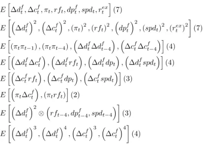
We use a total of 34 moment conditions to estimate the model parameters. These moments are explicitly listed in Table 2. They can be ordered into 6 groups. The first set is simply the uncon-ditional means of the Wt variables; the second group includes the second uncentered moments of

the state variables. In combination with the first moments above, these moments ensure that we are matching the unconditional volatilities of all the variables of interest. The third set of moments is aimed at identifying the autocorrelation of the fundamental processes. Because of the moving averagefilter applied to dividend and consumption growth, it is only reasonable to look at the fourth order autocorrelations. Because our specification implies complicated ARMA behavior for inflation dynamics, we attempt tofit both thefirst and fourth order autocorrelation of this series. The fourth set of moments concerns contemporaneous cross moments of fundamentals with asset prices and returns. As was pointed out by Cochrane and Hansen (1995), the correlation among fundamentals and asset prices implied by standard implementations of the consumption CAPM model can be much too high. We also include cross moments between inflation, the short rate, and consumption growth to help identify the ρπu parameter in the inflation equation and a potential inflation risk

premium.

Next, thefifth set of moments identifies higher order moments of dividend growth. This is crucial to ensure that the dynamics ofvt are identified by, and consistent with, the volatility predictability

of the fundamental variables in the data. Moreover, this helpsfit their skewness and kurtosis. Note that there are 34₋19 = 15over-identifying restrictions and that we can use the standard

J-test to test thefit of the model.

5

Estimation Results

This section describes the estimation results of the structural model, and characterizes thefit of the model with the data.

5.1

GMM Parameter Estimates

Table 2 reports the results of the above described estimation procedure. We start with dividend growth dynamics. First,utsignificantly forecasts dividend growth. Second, the conditional

volatil-ity of dividend growth,vt, is highly persistent with an autocorrelation coefficient of0.9795and itself

has significant volatility (σvv, is estimated as0.3288with a standard error of0.0785). This confirms

that dividend growth volatility varies through time. Further, the conditional covariance of dividend growth andvtis positive and economically large: σdv is estimated at0.0413 with a standard error

of0.0130.

The results for the consumption-dividend ratio are in line with expectations. First, it is very persistent, with an autocorrelation coefficient of0.9826(standard error0.0071). Second, the contem-poraneous correlation ofutwith∆dtis sharply negative as indicated by the coefficientσud which is

estimated at₋0.9226. In light of Equation (3), this helps to match the low volatility of consumption growth. However, because(1 +σud)is estimated to be greater than zero, dividend and consumption

growth are positively correlated, as is true in the data. Finally, the own volatility parameter for the consumption dividend ratio is 0.0127 with a standard error of just 0.0007, ensuring that the correlation of dividend and consumption growth is not unrealistically high.

The dynamics of the stochastic preference process, qt, are presented next. It is estimated to

be quite persistent, with an autocorrelation coefficient of 0.9787(standard error 0.0096) and it has significant independent volatility as indicated by the estimated value of σqq of 0.1753 (standard

error0.0934). Of great importance is the contemporaneous correlation parameter betweenqt and

consumption growth, σqc. Whileσqc is negative, it is not statistically different from zero. This

indicates that risk is indeed moving countercyclically, in line with its interpretation as risk aversion under a habit persistence model such as that of Campbell and Cochrane (1999) (further discussion below). What is different in our model is that the correlation between consumption growth and risk

aversion8 is₋0.37 instead of₋1.00in Campbell and Cochrane. The impatience parameterln (β)

is negative as expected and the γparameter (which is not the same as risk aversion in this model) is positive, but not significantly different from zero. The wedge between mean dividend growth and consumption growth,δ, is both positive and significantly different from zero.

Finally, we present inflation dynamics. As expected, past inflation positively affects expected inflation with a coefficient of 0.2404 (standard error 0.1407) and there is negative and significant predictability running from the consumption-dividend ratio to inflation.

5.2

Model Moments Versus Sample Data

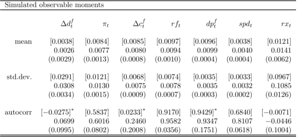
Table 2 also presents the standard test of the overidentifying restrictions. The overidentification test fails to reject, with a p-value of0.6234. However, there are a large number of moments beingfit and in such cases, the standard GMM overidentification tests are known to have low power infinite samples. Therefore, we examine thefit of the model with respect to specific moments in Tables 3 and 4.

Table 3 focuses on linear moments of the variables of interest: mean, volatilities and autocorre-lations. The model fits the data exceedingly well with respect to the unconditional means of all seven of the endogenous variables. This includes generating a realistic low mean for the nominal risk free rate of about 1% and a realistic equity premium of about 1.2% (all quarterly rates). The volatilities of the endogenous variables are also well matched to the data. The implied volatilities of both the financial variables and fundamental series are within one standard error of the data moment. Finally, the model is broadly consistent with the autocorrelation of the endogenous series. The (fourth) autocorrelation of filtered consumption growth is somewhat too low relative to the data. However, in unreported results we verified that the complete autocorrelograms of dividend and consumption growth implied by the model are consistent with the data. The model fails to generate sufficient persistence in the term spread but this is the only moment not within a two standard bound around the data moment. However, it is within a 2.05 standard error bound!

As explored below, the time varying volatility of dividend growth is an important driver of equity returns and volatility, and it is therefore important to verify that the model implied nonlinearities in fundamentals are consistent with the data. In Table 4, we determine whether the estimated model

8_{More specifically, the conditional correlation between ∆c}

t+1andqt+1whenvt andqt are at their unconditonal

is consistent with the reduced form evidence presented in Table 1, and we investigate skewness and kurtosis of fundamentals and returns. In Panel A, we find that the volatility dynamics for fundamentals are quite well matched. The model produces the correct sign in forecasting dividend and consumption growth volatility with respect to the short rate and the spread; only the volatility dynamics with respect to the dividend yield are of the wrong sign. However, for return volatility, all the predictors have the right sign, including the dividend yield.

Panel B focuses on multivariate regressions. This is a very tough test of the model as it implicitly requires the model to alsofit the correlation among the three instruments. Nevertheless, for consumption growth volatility the model gets all the signs right and every coefficient is within two standard errors of the data coefficient. The model also produces a fantastic fit with respect to time-variation in return predictability. However, thefit with respect to dividend growth volatility is not as stellar with two of three signs missed.

Panel C focuses on skewness and kurtosis. The model implied kurtosis of filtered dividend growth is consistent with that found in the data and the model produces a bit too much kurtosis in consumption growth rates. Equity return kurtosis is somewhat too low relative to the data, but almost within a 2 standard error bound. The model produces realistic skewness numbers for all three series. We conclude that the nonlinearities in the fundamentals implied by the model are reasonably consistent with the data.

6

Risk, Uncertainty and Asset Prices

In this section, we explore the dominant sources of time variation in equity prices (dividend yields), equity returns, the term structure, expected equity returns and the conditional volatility of equity returns. We also investigate the mechanisms leading to ourfindings.

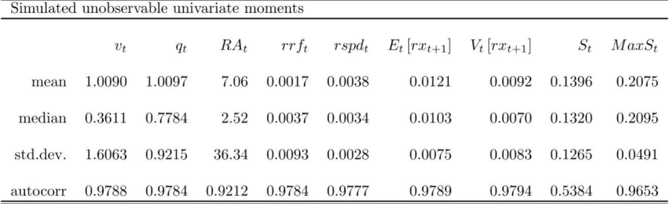
Tables 5 and 6 contain the core results in the paper. Table 5 reports basic properties of some critical unobserved variables, including vt and qt. Table 6 reports variance decompositions with

standard errors for several endogenous variables of interest and essentially summarizes the response of the endogenous variables to each of the state variables. Rather than discussing these tables in turn, we organize our discussion around the different variables of interest using information from the two tables.

6.1

Uncertainty and Risk

Table 5, Panel A presents properties of unobservable variables under the estimated model. First, note that ‘uncertainty,’vt, which is proportional to the conditional volatility of dividend growth is

quite volatile relative to its mean and is extremely persistent. These properties reflect the identifying information in the characteristics of the dividend yield, short rate and spread as well as the higher moments of fundamentals. Similarly, qt has significant volatility and autocorrelation. Because

local risk aversion,RAt, in this model is given byγexp (qt), we can examine its properties directly.

The median level of risk aversion in the model is 2.52, a level which would be considered perfectly reasonable by mostfinancial economists. However, risk aversion is positively skewed and has large volatility so that risk aversion is occasionally extremely high in this model.

Panel B of Table 5 presents results for means of the above endogenous variables conditional on whether the economy is in a state of expansion or recession. For this exercise, recession is defined as one quarter of negative consumption growth. Bothvtandqt(and hence local risk aversion) are

strongly counter-cyclical.

6.2

Uncertainty, Risk and the Term Structure

Panel A of Table 5 also displays the properties of the real interest rate and the real term spread. The average real rate is 17 basis points (68 annualized) and the real interest rate has a standard deviation of around90basis points. The real term spread has a mean of38basis points, a volatility of only28 basis points and is about as persistent as the real short rate. In Panel B, we see that real rates are pro-cyclical and spreads are counter-cyclical.

Panel C of Table 5 shows that uncertainty tends to depress real interest rates, while positive risk aversion shocks tend to increase them. In the theoretical section, we derived that the effect ofqton

real interest rates is ambiguous depending on whether the consumption smoothing or precautionary savings effect dominates. At our parameter values, the consumption smoothing effect dominates. The effect ofvtis entirely through the volatility of the pricing kernel and represents a precautionary

savings motive. Hence, the correlation between real rates and qt is actually positive, while the

correlation between real rates andvt is negative. Overall, real rates are pro-cyclical because vt is

strongly counter-cyclical.

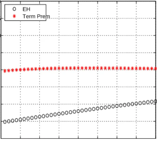
As we discussed in the theoretical section, if the expectations hypothesis were to hold, mean reversion would imply that the effect of either variable on the spread would be the opposite sign of its effect on the interest rate level. Figure 1 decomposes the exposures of both the real interest rate and the spread tovt andqtinto an expectations hypothesis part and a term premium part and does so for

various maturities (to 40 quarters). The exposure tovtis negative and weakens with horizon leading

to a positive EH effect. Becausevt has little effect on the term premium, the spread effect remains

positive. Hence, when uncertainty increases, the term structure steepens and vice versa.

Figure 1 also shows whyqthas a positive effect on the real term spread, despite the EH effect being

negative. Yields at long maturities feature a term premium that is strongly positively correlated withqt. In the theoretical section, we derived that the sign of the term premium only depends on

φrq which is positive: because higher risk aversion increases interest rates (and lowers bond prices)

at a time when marginal utility is high, bonds are risky.

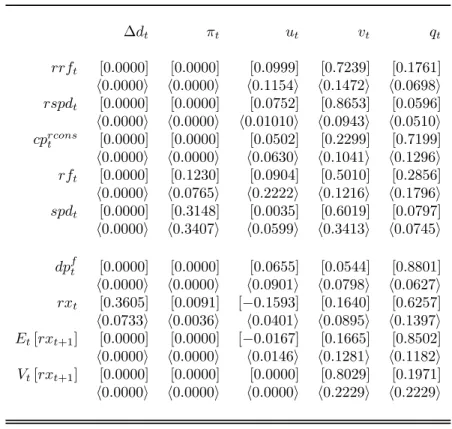
In Table 6, we report the variance decompositions. While three factors (ut, vt, and qt) affect

the real term structure, vtaccounts for the bulk of its variation. An important reason for this fact

is that vt is simply more variable than qt. The most interesting aspect of the results here is that

qtcontributes little to the variability of the spread, so that qtis mostly a level factor not a spread

factor, whereas uncertainty is both a level and a spread factor. When we consider a real consol, we

find thatqtdominates its variation. Because consol prices reflect primarily longer term yields, they

are primarily driven by the most persistent level factor, which isqt, through its effect on the term

premium.

For the nominal term structure, inflation becomes an important additional state variable ac-counting for about 12% of the variation in the nominal interest rates. However, inflation is an even more important spread factor accounting for about 31% of the spread’s variability. What may be surprising is that the relative importance of qt increases going from the real to nominal

term structure. The reason is the rather strong positive correlation between inflation andvt, which

arises from the negative relation between inflation and the consumption dividend ratio, that ends up counterbalancing the negative effect of vton real interest rates.

6.3

Uncertainty, Risk, and Equity Prices

Here we start with the variance decompositions for dividend yields and equity returns in Table 6. For the dividend yield, qt dominates as a source of variation. The contribution of qt to variation

in the dividend yield is almost 90%. To see why, recall first that qt only affects the dividend

yield through its effect on the term structure of real interest rates (see Proposition 4). Under the parameters presented in Table 2, the impact ofqton real interest rates is positive at every horizon

and therefore it is positive for the dividend yield as well. Formally, under the parameters of Table 2,Fbn in Proposition 3 is negative at all horizons.

Next, consider the effect of vt on the dividend yield. Uncertainty has a ‘real consol effect’

and a ‘cash-flow risk premium’ effect which offset each other. We already know that vt creates

a strong precautionary savings motive, which decreases interest rates. All else equal, this will serve to increase price-dividend ratios and decrease dividend yields. However, vt also governs the

covariance of dividend growth with the real kernel. This risk premium effect may be positive or negative, but intuitively the dividend stream will represent a risky claim to the extent that dividend growth covaries negatively with the kernel. For instance, if dividend growth is low in states of the world where marginal utility is high, then the equity claim is risky. In this case, we would expect high vt to exacerbate this riskiness and depress equity prices when it is high, increasing dividend

yields. As we discussed in section 5.5, σqc contributes to this negative covariance. On balance,

these countervailing effects ofvton dividend yield largely cancel out, so that the net effect ofvton

dividend yields is small. This shows up in the variance decomposition of the dividend yield. On balance, qt is responsible for the overwhelming majority of dividend yield variation, and is highly

positively correlated with it. The negative effect of ut arises from its strong negative covariance

with dividend growth.

Looking back to panel C in Table 5, while increases in qthave the expected depressing effect on

equity prices (a positive correlation with dividend yields), increases invt do not. This contradicts

thefindings in Wu (2001) and Bansal and Yaron (2004) but is consistent with early work by Barsky (1988) and Naik (1994). Because the relation is only weakly negative, there may be instances where our model will generate a classic “flight to quality” effect with uncertainty lowering interest rates, driving up bond prices and depressing equity prices.

Next notice the determinants of realized equity returns in Table 6. First, over 30% of the variation in excess returns is driven by dividend gr