Error-tolerant Resource Allocation and Payment
Minimization for Cloud System
Sheng Di,
Member, IEEE,
and Cho-Li Wang,
Member, IEEE
Abstract—With virtual machine (VM) technology being increasingly mature, compute resources in Cloud systems can be partitioned in fine granularity and allocated on demand. We make three contributions in this paper: (1) We formulate a deadline-driven resource allocation problem based on the Cloud environment facilitated with VM resource isolation technology, and also propose a novel solution with polynomial time, which could minimize users’ payment in terms of their expected deadlines. (2) By analyzing the upper bound of task execution length based on the possibly inaccurate workload prediction, we further propose an error-tolerant method to guarantee task’s completion within its deadline. (3) We validate its effectiveness over a real VM-facilitated cluster environment under different levels of competition. In our experiment, by tuning algorithmic input deadline based on our derived bound, task execution length can always be limited within its deadline in the sufficient-supply situation; the mean execution length still keeps 70% as high as user-specified deadline under the severe competition. Under the original-deadline-based solution, about 52.5% of tasks are completed within 0.95∼1.0 as high as their deadlines, which still conforms to the deadline-guaranteed requirement. Only 20% of tasks violate deadlines, yet most (17.5%) are still finished within 1.05 times of deadlines.
Keywords—VM-multiplexing, Resource Allocation, Convex Optimization, Prediction Error Tolerance, Payment Minimization
F
1
INTRODUCTION
Cloud computing [1], [2] has emerged as a compelling paradigm for the deployment of ease-of-use virtual envi-ronment on the Internet. One typical feature of Clouds is its pool of easily accessible virtualized resources (such as hardware, platform or services) that can be dynamically reconfigured to adjust to a variable load (scale). All the resources provisioned by Cloud system are supposed to be under a payment model [2], in order to avoid users’ over-demand of their resources against their true needs. Each task’s workload is likely of multiple dimensions. First, the compute resources in need may be multi-attribute (such as CPU, disk-reading speed, network bandwidth, etc.), resulting in multi-dimensional execu-tion in nature. Second, even though a task just depends on one resource type like CPU, it may also be split to multiple sequential execution phases, each calling for a different computing ability and various price on demand, also leading to a potentially high-dimensional execution scenario.
The resource allocation in Cloud computing is much more complex than in other distributed systems like Grid computing platform. In a Grid system [3], it is improper to share the compute resources among the multiple applications simultaneously running atop it due to the inevitable mutual performance interference among them. Whereas, Cloud systems usually do not provision physical hosts directly to users, but leverage virtual resources isolated by VM technology [4], [5], [6]. • S. Di is currently a post-doctor researcher at INRIA, Grenoble, France, and C.L. Wang is with the Department of Computer Science, The University of Hong Kong, Hong Kong.
Not only can such an elastic resource usage way adapt to user’s specific demand, but it can also maximize resource utilization in fine granularity and isolate the abnormal environments for safety purpose. Some suc-cessful platforms or cloud management tools leveraging VM resource isolation technology include Amazon EC2 [7] and OpenNebula [8]. On the other hand, with fast development of scientific research, users may propose quite complicated demands. For example, users may wish to minimize their payments when guaranteeing their service level such that their tasks can be finished before deadlines. Such a deadline-guaranteed resource allocation with minimized payment is rarely studied in literatures. Moreover, inevitable errors in predicting task workloads will definitely make the problem harder.
Based on the elastic resource usage model, we aim to design a resource allocation algorithm with high prediction-error tolerance ability, also minimizing users’ payments subject to their expected deadlines.
Since the idle physical resources can be arbitrarily partitioned and allocated to new tasks, the VM-based divisible resource allocation could be very flexible. This implies the feasibility of finding the optimal solution through convex optimization strategies [9], unlike the traditional Grid model [10] that relies on the indivisible resources like the number of physical cores. However, we found it is inviable to directly solve the necessary and sufficient condition to find the optimal solution, a.k.a., Karush-Kuhn-Tucker (KKT) conditions [9]. Our first contribution is devising a novel approach (with only
O(n·R2)time complexity) to solve the problem, where
Rdenotes the number of execution dimensions andnis the system scale (the number of compute nodes).
often subject to the precise prediction of task’s charac-teristic (or execution property), which is nontrivial to realize in practice. Accordingly, as the state-of-the-art, we further analyze our algorithm’s optimality approxima-tion ratio given the possibly wrong predicapproxima-tions of tasks’ execution properties. In particular, we will try to answer such a question: when application’s characteristic is pre-dicted with certain levels of errors, will the application’s final execution length (a.k.a., execution time) violate (or surpass) its deadline? If yes, what is the ratio of the final execution time to its deadline? These theoretical results will be significantly valuable to the guarantee of user’s service level in practice. In fact, by setting a relatively stricter deadline properly based on our derived approx-imation ratio, each task can be guaranteed to be finished within its original deadline even though task properties cannot be predicted accurately.
In addition to the above theoretical contribution, we further confirm the effectiveness of our solutions by implementing a set of advanced web services that are based on complex matrix-operations, over a real cluster environment with 60 virtual machines. All the theoretical conclusions are confirmed with our experiments. Specif-ically, in the situation with relatively sufficient resources, the worst-case tasks under thestricter-deadline based allo-cationonly take as about 0.75 times as their deadlines to complete, as compared to the 1.2 times of the deadlines under the originaluser-predefined deadline based allocation. We also observe that in the competitive environment, the latter algorithm performs much more stable than the former instead, which means that the latter tolerates the resource competition better. We also confirm the effectiveness of our solution via the distribution of the number of tasks with respect to execution times and user payments: in the competitive situation, majority of tasks can be guaranteed to be completed within deadlines.
The rest of the paper is organized as follows: In Section 2, we formulate our problem based on the Cloud scenario which supports elastic divisible resource cus-tomization. In Section 3, we first discuss the complexity of the modeled problem in brief, and then formally describe a novel algorithm, which can minimize user’s payment based on task’s preset execution deadline. In Section 4, we intensively derive the lower bound and upper bound of execution time for the situation with the possibly skewed predictions on tasks’ properties as compared to the deadlines. We rigorously implement our algorithm and analyze experimental results on a real-cluster setting in Section 5. We discuss the related works in Section 6 and conclude with future work in Section 7.
2
PROBLEM
FORMULATION
In Cloud systems, the Cloud proxy (a.k.a., server) con-tinually receives and responds to user requests (or tasks) with customized requirements (or virtual machines). All tasks will be handled based on their priorities (like Google task scheduler [11]) or in terms of First-Come-First-Serve (FCFS) policy when the tasks are of the same
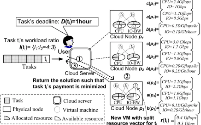
priorities (like [12]). Each task’s execution may involve multi-dimensional resources, such as CPU and disk I/O. A data mining task, for example, usually needs to load a large set of data from disk before or in the middle of its computation. Eventually, such a task may store its computation results onto the local disk or a public server through network. Fig. 1 illustrates the procedure in processing such a task (denotedti). Suppose the task’s execution times cost on computation and disk process-ing are predicted as 4 hours and 3 hours respectively. Upon receiving the request, the scheduler checks the pre-collected availability states of all candidate nodes, and estimates the minimal payment of running the task within its deadline on each of them (i.e., Step 1 in the figure). The host (Nodep3 shown in Fig. 1) that requires
the lowest payment will run the task via a customized VM instance with isolated resources (Step 2 in Fig. 1). Specifically, the VM will be customized with such a CPU rate (e.g., 0.4 Gflops) and disk I/O rate (e.g., 0.3 Gbps) that the task can be finished within its deadline (D(ti)=1 hour in the example) and its user payment can also be minimized meanwhile. Finally (Step 3), its computation results (or feedbacks) will be returned to users.
i Tasks Cloud Server 1 3 Cloud Node p3 User
Task Cloud server Virtual machine Physical node
Allocated resource Available resource
CPU IO-BW
CPU CPU
Cloud Nodep1
Cloud Nodep2 Task’s deadline: D(ti)=1hour
Task ti’s workload ratio l(ti)= {l1:l2=4:3} CPU=1.2Gflops a(p1)= b(p1)= IO=0.5Gbps IO-BW IO-BW CPU=0.5$/Gflops/hr IO=0.1$/Gb/hour 1.2 0.5 CPU=1.5Gflops a(p2)= b(p2)=CPU=0.2$/Gflops/hr IO=0.2$/Gb/hour IO=0.8Gbps CPU=1.0Gflops a(p3)= b(p3)=CPU=0.1$/Gflops/hrIO=0.2$/Gb/hour IO=1.1Gbps t1 t2 t3 t4 t5 t6 ti 2
New VM with split resource vector for ti
r(ti) 0.4 Gflops 0.3 Gbps = CPU=2.2Gflops c(p3)= IO=2.2Gbps CPU=2.4Gflops c(p1)= IO=1Gbps CPU=3.0 Gflops c(p2)= IO=1.2 Gbps
Return the solution such that task ti’s payment is minimized
Fig. 1: Resource Allocation in Cloud System
Suppose there are n compute nodes (denoted by pi, where 1≤i≤n). Since all the resources are managed centrally, the availability state of each resource within any recent or later period can be predicted prior, for executing any given task with multiple execution di-mensions. For any particular task with R execution dimensions, we use Π to denote the whole set of dimensions and c(pi)=(c1(pi) , c2(pi) ,· · ·, cR(pi))T as node pi’s capacity vector on these dimensions (In the paper, we use bold-type to indicate a vector). In Fig. 1, for example, node p1’s physical capacity vector is
c(p1)={CPU=2.4Gflops,disk IO=1Gbps}.
Any user’s task is denoted as ti, where 1≤i≤m, and m refers to the total number of submitted tasks. Each task has a multi-dimensional workload vector, de-noted by l(ti)=(l1(ti),l2(ti),· · ·, lR(ti))T, which needs to be finished before the task’s deadline. We denote the resource vector allocated to ti as r(ti) = (r1(ti), r2(ti),
· · · , rR(ti))T, where rk(ti) (k=1,2,· · ·,R) refers to the resource amount on kth execution dimension isolated
by hypervisor/virtual machine monitor(VMM) for the task’s execution. Node pi’s availability vector (denoted
a(pi)) along the multiple dimensions is calculated by
c(pj) − ∑tirunning on pjr(ti). For example, node p1 in
Fig. 1 is running two VMs that are allocated with half of the total physical resources, so its availability vector
a(p1)={CPU=1.2Gflops,disk IO=0.5Gbps}. If there are no
workloads being executed simultaneously for a particu-lar task, its total execution time will be the sum of the individual processing times on different dimensions. If the execution of the workloads overlap, however, the task’s completion time would be shorter. Accordingly,
ti’s final execution time (denoted asT(ti)) is definitely confined within such a range [max(lk
rk),
∑R
k=1
lk
rk]. For
simplicity, we denote taskti’s execution time as Equation (1) (affine transformation of∑Ri=1
lk
rk), whereθdenotes a
constant coefficient. Such a definition specifies a defacto broad set of applications each with multiple execution dimensions. The typical example is a single job with multiple sequentially interdependent tasks or some pro-gram with distinct execution phases each relying on independent compute resources (where θ= 1).
T(ti) =θ ∑R k=1 lk(ti) rk(ti) , where θ∈[max( lk rk) ∑R k=1 lk rk ,1] (1)
For any Cloud system, the resources provisioned are usually set with a price vector denoted as b(pi)=(b1(pi),
b2(pi),· · · , bR(pi))T along R dimensions. bk(pi) (1 ≤ k
≤R) denotes the per-time-unit price that the consumers need to pay for the consumption of the kth dimension onpi. Each taskti is set with a deadline (denotedD(ti)) for its execution and the payment is expected to be minimized under our algorithm.
In our Cloud model, any task will be executed on one or more virtual machines with user-reserved re-sources and the payment is calculated based on the cus-tomized resource (a.k.a., pay-by-reserve policy). Adopt-ing such a pricAdopt-ing policy is driven by three reasons. Firstly, the efficiencies of many applications usually rely on multiple resources but it is non-trivial to precisely evaluate the exact amount of their consumption sep-arately on individual resources. Secondly, quite a few users prefer to reserving resources for tolerating us-age burst and guaranteeing their service levels. Lastly, the alternative pricing policy, pay-as-you-consume, is rather simple because its payment is always fixed (=
θ∑Rk=1(bk(ps)·rk(ti)rlk(ti)
k(ti))=θ
∑R
k=1bk(ps)·lk(ti)) regardless of the resource allocation.
Based on the pay-by-reserve policy, task ti’s total payment will be calculated via Equation (2), where
ps refers to ti’s execution node. The mean price (i.e.,
1
Rb(ps) T·r(t
i)) will be used as the pricing unit over time, for computing user’s payment. Such a design can be con-sistent with our pay-by-reserve model, and also prevent users from feeling too costly when their applications’ execution cannot overlap at different dimensions.
P(r(ti)) =
1 Rb(ps)
T·
r(ti)·T(ti) (2)
In this paper, we might omit the notations ti and pi if thus would not cause ambiguity. For instance, lk(ti),
r(ti),bk(pi),a(pi)andD(ti)may be substituted bylk,r,
bk,a, andD respectively, in the following text.
Our research could be briefly summarized as the following convex optimization format: for any task ti with its workload vector l(ti), given a set of candidate execution nodes (ps, s=1,2,· · ·,n), how to select ps and split resources such thatti’s payment (i.e., Equation (2)) is minimized, subject to the constraints (3) and (4).
M in P(r(ti))
s.t.
T(ti)≤D(ti) (3)
r(ti)≼a(ps) (4)
3
OPTIMAL
RESOURCE
ALLOCATION
In this section, we will first analyze the problem men-tioned above, and then propose our optimal solution.
By combining Equation (1) and Equation (2), it is easy to verify that∀rk,∂2P(r(ti)) ∂r2 k = θ R(− 2bklk r2 k +2lk r3 k ∑R i=1biri)>0, thus the target functionP(r(ti))is convex, which means that there must exist a minimal extreme point.
Based on the convex optimization theory [9], the La-grangian function of the problem could be formulated as Equation (5), whereλandµ1,µ2,· · ·,µRare correspond-ing Lagrangian multipliers. Note that θ is a constant defined in Equation (1) andris the abbreviation ofr(ti) as stated above. F1(r)=R1( R ∑ k=1 bkrk)(θ R ∑ k=1 lk rk)+λ(θ R ∑ k=1 lk rk−D)+ R ∑ k=1 µk(rk−ak) (5) Accordingly, we could get the Karush-Kuhn-Tucker (KKT) conditions [9] (i.e., the necessary and sufficient condition of the optimization) as below:
λ≥0, µk ≥0, k= 1,2· · ·, R R ∑ i=1 θli ri ≤D λ(θ R ∑ i=1 li ri −D) = 0 rk ≤ak(ps), k= 1,2,· · ·, R;s= 1,2,· · ·, n µk(rk−ak(ps)) = 0, k=1,2,· · ·, R;s=1,2,· · ·, n ∂F1 ∂rk= 1 R ((∑R i=1 biri ) ·−lk r2 k +bk· R ∑ i=1 li ri+ −λlk r2 k +µk ) = 0, k= 1,2,· · ·, R (6)
In other words, as long as we can find such an allocation case (r=(r1, r2,· · ·, rR)T) to satisfy the above conditions simultaneously, we can set it as the opti-mal solution of the deadline-driven payment-minimized problem. However, it is non-trivial to do that, because the last condition (∂F1
∂rk=0) cannot be directly solved.
Whereas, we exploit a novel algorithm with polynomial time complexity (n·R2) to allocate resource, which can
be proved to satisfy the KKT condition listed above. Our algorithm is designed based on such a discovery: if we do not consider the limit of resource capacities (i.e condition (4)), the problem can be directly solved using Lagrangian multiplier method. As follows, we will
first derive the optimal solution to the problem with unbounded capacities (i.e., without the condition (4)) in Theorem 1. And then, we will describe our algorithm by recursively using Theorem 1 to search the resource allocation case that satisfies the whole KKT condition (6), in polynomial time.
Theorem 1: For a specific task ti, in order to minimize
P(r(ti))subject to the constraint (3), the optimal resource vectorr(∗)(t
i)is Equation (7), wherek=1, 2,· · ·,R. (Note that r(∗)(t
i) is not subject to Inequality (4), unlike the notation r∗(ti)that takes into account this inequality.)
rk(∗)(ti) = ( θ D ∑R j=1 √ ljbj ) √ lk bk (7)
Proof: As mentioned previously, the target function is convex, thus there must exist the minimal extreme point. In order to simplify the target function (i.e., Equa-tion (2)), we fix the task’s execuEqua-tion time to be T (≤D), which also satisfies the problem’s conditions. Then, the target function could be converted to Equation (8).
P(r) =TR·∑kR=1bkrk, where T ≤ D (8)
The corresponding Lagrangian function is shown be-low: F2(r) = TR· ∑R k=1bkrk+λ(θ ∑R k=1 lk rk−D) (9)
Based on the Lagrangian multiplier method, ∂F2
∂rk = 0
(where k=1,2,· · ·,R) constructs a set of necessary condi-tions for getting the optimal solution (i.e., Equation (10) must hold, where λis a constant).
λθR/T =bkr2k/lk (10)
According to Equation (10), we can easily get Equation (11),∀j, k(1≤j̸=k≤R).
r2kbk/lk=r2jbj/lj (11)
That is, Equation (12) is the sufficient and necessary condition of the optimal solution, s.t. a given deadline.
r1:r2:· · ·rR= √ l1/b1: √ l2/b2:· · ·: √ lR/bR (12)
In order to save the resource utilized by the current task as much as possible, the optimal allocation should make ∑Ri=1
li
ri equal to D. In fact, for any resource
allocation r(ti) meeting Equation (12) while
∑R
i=1
li
ri <
D, there must exist another solution with lower resource allocationr(ti)′(i.e.,r′(ti)≼r(ti)) such that it also satisfies Equation (12). Hence, the task ti’s optimal resource al-location should make∑Rk=1
lk
rk =D, then, by combining
this equation, we can calculate the the optimal resource vector to be allocated as Equation (7).
Remark: With unbounded resource availabilities, there
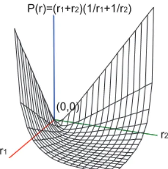
will be no any constraint to the problem of minimizing the target function P(r). Based on the above analysis, there are infinite number of optimal stationary points, whose sufficient and necessary conditions are Equation (12). For vivid illustration, we show the graph of a simple case in Fig. 2, where b=(1,1)T and l=(1,1)T. From this figure, we can observe that these exist the minimal extreme points and the number of them is infinitive, along the line{r1=r2andP(r)=4}. This result
is consistent with the Equation (12).
(0,0)
r1
r2
P(r)=(r1+r2)(1/r1+1/r2)
Fig. 2: The function Graph of A Simple Case
Formula (7) presents the resource share vector r(∗)
gained by ti such that its payment and the resource utilization can be both minimized within its execution deadline (i.e., Formula (3)). Considering the constraint (4),r(∗)is right the optimal solution as long asr(∗)≼a(p
s). However, if r(∗) does not fully satisfy the constraint
(4) (i.e., ∃ k: r(k∗)>ak(ps)), r(∗) should not be a feasible solution. As one contribution, we propose an efficient algorithm (Algorithm 1) to determine the optimal solu-tion subject to the constraint (4) with the provable time complexityO(n·R2).
Definition 1: For any taskti, based on a subsetΓ(⊆Π), CO-STEP(Γ,C) is defined as the procedure of computing the optimal solution of minimizing P(rΓ(ti)) subject to the constraint (13) by using convex optimization (similar to the proof of Theorem 1), whereCdenotes a deadline andrΓ(ti)(=(r1, r2,· · ·, rR)T) denotes the resource shares gained byti on the execution dimension setΓ.
θ∑R
i=1
li
ri ≤
C (13)
We devise Algorithm 1 for minimizingP(r(ti))subject to the constraints (3) and (4), as shown below.
Algorithm 1 OPTIMALALLOCATIONALGORITHM
Input:D(ti);Output: execution nodeps,r∗(ti)
1: for(each candidate nodeps)do
2: Γ=Π,C =D(ti),r∗=Φ(empty set);
3: repeat
4: r(Γ∗)(ti, ps)= CO-STEP(Γ,C); /*Compute optimalronΓ*/ 5: Ω = {dk|dk∈ Γ & r
(∗)
k (ti, ps)>ak(ps)}; /*select elements
violating constraint (4)*/ 6: Γ=Γ\Ω; /*Γtakes awayΩ*/ 7: C=C−θ∑d k∈Ω lk ak; /*UpdateC*/ 8: r∗(ti, ps)=r∗(ti, ps)∪{rk∗=ak(ps)|dk∈Ω &ak(ps)isdk’s upper bound}; 9: until(Ω = Φ); 10: r∗(ti, ps)=r∗(ti, ps)∪r(Γ∗)(ti, ps); 11: end for
12: Select the smallestP(ti)by traversing the candidate solution set;
13: Output the selected nodepsand resource allocationr∗(ti, ps);
In this algorithm, line 4 executes CO-STEP(Γ,C) in order to find the optimalr(Γ∗)(ti, ps), under the assump-tion without constraint (4). If r(Γ∗)(ti, ps)completely sat-isfies the constraint (4) (i.e., Ω=Φ), then rΓ(∗)(ti, ps) is the local optimal resource allocation for ti to be run on ps; otherwise, let the resource shares (rk(ti),where
upper bound (i.e., ak(ps)) and take the corresponding execution dimensions (i.e., Ω) away from Γ, then, C
= C −θ∑dk∈Ω lk
ak for the remaining dimensions. The
process will go on until the computed optimal resource shares on the remaining dimensions satisfy the con-straint (4). Since the time complexity of CO-STEP(Γ,C) isO(|Γ|), the number of computation steps of line 2∼10 in Algorithm 1 in the worst case is ∑Ri=0−1(R−i), thus
the total time complexity of Algorithm 1=O(n·R2). Based on the Algorithm 1, it is obvious that the local optimal resource allocation for ti to be executed on a specified node ps is the most crucial part. In fact, the final outputted resource allocation solution of the whole algorithm will be globally optimal around the whole system as long as each local process on a specified node (line 2∼10) can be proved as optimal resource alloca-tion. Consequently, we will intensively discuss the local divisible-resource allocation by specifying a particular execution node, in the following text.
Theorem 2: Given a submitted task ti with its load vector l(ti)and a deadline D(ti) and a particular node
ps with its resource price vector b(ps), thenthe output after running the line 2∼10 of Algorithm 1 (i.e.,r∗(ti, ps) is optimal for minimizing ti’s payment (i.e., P(r(ti))), subject to the constraints (3) and (4).
Main idea: We will prove that ther∗(ti, ps)satisfies KKT conditions (i.e., Formula (6)).
Proof:
At the beginning, the algorithm executes the CO -STEP(Π,D(ti)) and the output is denoted r
(∗)
Π . Since r (∗) Π
is derived from Definition 1 and Theorem 1, r(Π∗) must
satisfy Equation (12) and θ∑Ri=1 li
ri=D, then if we let
µk=0 for anyk, there must exist an assignment such that all the conditions in Formula (6) hold except forr(k∗)≤ak. Accordingly,r∗=r(Π∗)as long asr (∗) k ≤akfor allr (∗) k s inr (∗) Π .
If r(Π∗) cannot satisfy all the R inequalities (r∗k≤ak, where k=1, 2, · · · , R), we need to further adjust the solution r(Π∗) to find the one completely satisfying the
condition (6). In Algorithm 1, at this moment, all ther(k∗)s such thatr(k∗)>ak will be selected and set toak. Without loss of generality, assuming there are h1 such resource
shares and they are denoted asr1,r2,· · ·,rh1. Obviously,
each selected rk must satisfy µk·(rk −ak)= 0 because
rk=ak. On the other hand, Algorithm 1 will continue to execute CO-STEP(Γ,C) on the rest R−h1 dimensions,
where C=D(ti)−θ
∑h1
k=1
lk
rk. Likewise, all the R−h1 new
resource shares (each denoted byrk,k=h1+1,· · ·,R) must
also satisfy rh1+1 : rh1+2 :· · · : rR = √ lh1 +1 bh1 +1 : √ lh1 +2 bh1 +2 : · · · : √ lR bR, and ∑R i=1 li
ri=D, thus if each of them meets
the condition rk≤ak, the R −h1 new resource shares
and the previously selected h1 will together compose
the solution satisfying the condition (6). If there are still
h2 (0<h2≤R−h1) new resource shares violating rk≤ak in this round, Algorithm 1 will continue the adjustment until the Hth round such that either all the R−∑Hi=1hi remaining resource shares can satisfyrk≤ak or there are
no remaining resource dimensions in Γ. In the former case, we can easily verify that all theR resource shares satisfy the condition (6) simultaneously, composing an optimal solution; for the latter case, we could conclude that θ∑Ri=1 li
ai ≥D, then there does not exist a feasible
resource allocation to run the task within the specified deadline. In this situation,r∗=a=(a1, a2,· · ·, aR)T will get the execution time closest to the deadline, and it will serve as the final solution.
Although Algorithm 1 is proved optimal for minimiz-ing the payment cost within user-defined deadline for his/her task, the deadline still may not be guaranteed due to two factors, either bounded available resources or inaccurate workload vector information about the task. We propose the following lemma, which provides a necessary and sufficient condition of guaranteeing the task’s deadline given accurate prediction and relatively sufficient resources. In next section, we will discuss how to guarantee task’s deadline when performing the Algorithm 1 with even inaccurate workload vector.
Lemma 1: Given a taskti’s workload vectorl(ti)=(l1,
l2, · · · , lR)T and its deadline D(ti), and a candidate execution nodeps, then ti can be executed within D(ti) if and only if (i.e.,⇔) Inequality (14) holds.
∑R j=1 lj(ti) aj(ps) ≤D(ti) (14) Proof:
To prove ⇐: If Inequality (14) holds, it is obvious
there must exist a viable resource allocationr(ti)(≼a(ps)), such that∑Rj=1
lj(ti)
aj(ps)=D(ti). Hence,tican be executed
within D(ti).
To prove ⇒: Ifti can be executed withinD(ti), there
must exist a viable resource allocation r(ti) such that
∑R
j=1
lj
rj ≤D(ti)and r(ti)≼a(ps). Assuming Inequality
(14) does not hold at the moment, i.e., ∑Rj=1 lj(ti)
aj(ps) >
D(ti), then, we could derive Inequality (15).
∑R j=1 lj(ri) rj(ps) <∑R j=1 lj(ti) aj(ps) (15) Accordingly, we can derive that there must exist a dimension for exampledksuch thatrk(ti)≥a(ps), which contradicts to the previous assumption that r(ti) is a viable solution (r(ti)≼a(ps)).
4
OPTIMALITY
ANALYSIS WITH
INACCURATE
INFORMATION
In this section, we focus on such a question: what is the final upper bound of task execution length as compared to its predefined deadline D, when running it using the resource vector allocated under Algorithm 1 with inaccurately predicted workload information?
4.1 Problem Description
Although Algorithm 1’s output is proved optimal, such a result relies on a strong condition, i.e., accurate task’s workload vector. That is, each user needs to precisely
predict the execution property (i.e., workload ratio) for his/her task, before constructing the resource alloca-tion with minimized payment for its execualloca-tion under a user-specified deadline. In some cases, the execution property could be easily estimated accurately. For in-stance, we can decide the workload ratio between the data to be read/written from/to disk and those to be downloaded/uploaded via network by comparing their data sizes. In many other cases, however, the execution property cannot be accurately estimated, such as computation-intensive applications whose execution times highly depends on the CPU-cycles to consume.
Definition 2: Suppose a task ti’s real workload vector isl(ti), while its workload vector used by our algorithm isl′(ti)subject to the Inequality (16), whereαandβ are the lower bound and upper bound for the estimation ratio specified by user based on experiences or particular workload prediction methods such as [13], [14], [15].
α≤ l
′
k(ti)
lk(ti)≤
β, k= 1,2,· · ·R (16) To illustrate the above definition, an example is given. Assuming the task ti’s real workload ratios range in [0.125, 1], and the workload vector l′(ti)used by Algo-rithm 1 will be set based on the task’s historical execution records. Suppose each elementl′k(ti)(k= 1,2,· · ·R) will be set to 0.25 if the corresponding true workload fluctu-ates in [0.125, 0.5] and set to 0.75 if the true workload ranges within (0.5, 1]. Then, we could get Inequality (17) below, where α=0.125 0.25=0.5 andβ= 0.5 0.25=2. 0.5≤l ′ k(ti) lk(ti) ≤ 2, k= 1,2,· · ·R (17) Using the inaccurate prediction l′(ti) to perform the Algorithm 1, it is obvious that ti’s real execution time may surpass the expected execution deadline D(ti). Hence, one question is what the worst performance will get when using l′(ti) instead of l(ti), compared to the expected deadline D(ti).
4.2 Deadline Extension Ratio with Skewed Estima-tion of ExecuEstima-tion Property
For simplicity of description, we denote r∗E (=(rE∗1,rE∗2,
· · ·, r∗ER)T) and T∗ E (=θ
∑R
k=1
lk
rEk∗ ) as the output of Al-gorithm 1 with the skewed workload prediction and the corresponding execution time, respectively (E here implies “Estimation with error”). Similarly, we denote
rI∗(=(rI∗1,rI∗2,· · ·,r∗IR) T) andT∗ I (=D=θ ∑R k=1 lk r∗Ik) as the output with real workload vector and the correspond-ing execution time, respectively (I here indicates “Ideal case”). Hence, our objective is to determine the upper bound of TE∗
TI∗, a.k.a., deadline extension ratio.
We partition the situation that Algorithm 1 would face to two categories, where r(E∗) refers to the optimal resource allocation with the constraint (4) (unlike the notation r∗E): • r∗E(ti)=r (∗) E (ti). • r∗E(ti)̸=r (∗) E (ti).
The first situation indicates that in terms of the skewed estimation of workload ratios, all the resource shares calculated by the initial CO-STEP in Algorithm 1 are always no greater than the corresponding capacities. That is, it is equal to the situation with the assumption that Inequality (18) holds.
r(E∗)(ti)≼a(ps) (18) In contrast, the second one means that the initial CO -STEPcannot fulfill the above condition, and the optimal allocation cannot be found unless a few more adjustment steps (line 5∼8 of Algorithm 1).
As follows, we will first derive taskti’s execution time upper bound for the first category (i.e., Theorem 3), and then discuss the upper bound (i.e., Theorem 4) for the more generic case including the second category.
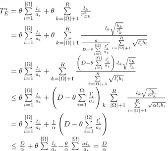
Theorem 3: Given a submitted task ti with a prede-fined deadlineD(ti), a candidate execution nodepswith unbounded resource capacity and a resource price vector (denoted b(ps)), and a skewed workload vector l′(ti) subject to Inequality (16), then the bound of execution time must satisfy Inequality (19), under the resource allocationr(E∗). 1 β ·D(ti)≤T (∗) E (ti)≤ 1 α·D(ti) (19) Proof: TE(∗)=θ R ∑ k=1 lk rEk(∗) =θ R ∑ k=1 lk ( θ D R ∑ i=1 √ l′ibi )√ l′k bk = D R ∑ i=1 √ l′ibi ∑R k=1 lk√√bk lk′ ≤ D √ α· 1 √ α· R ∑ k=1 √ lkbk R ∑ i=1 √ libi = Dα
The key of the above proof is based on the Inequality (16). Similarly, According to Inequality (16), we can also deriveTE(∗)≥ Dβ.
Accordingly, Inequality (19) holds. It is easy to see that Inequality (19)’s bound is tight. Considering such a case:
∀k,l′k(ti)=αlk(ti), thenT
(∗)
E will be equal to D α.
Theorem 4: Given a submitted task ti with a prede-fined deadline D(ti), a candidate execution node ps with a limited available resource vector (a(ps)) and price vectorb(ps), and a skewed workload vectorl′(ti)subject to Inequality (16), if Inequality (14) holds,thenunder the resource allocationr∗E, the bound of execution time must conform to Inequality (20). 1 β ·D(ti)≤T ∗ E(ti)≤ 1 α·D(ti) (20)
Proof:Without loss of generality, we denoteΩto be the set of resource dimensions accumulated by Line 5 of Algorithm 1, and the corresponding dimensions’ indexes are 1, 2, · · ·, |Ω|. That is, r∗1=a1, r2∗=a2, · · ·, r|∗Ω|=a|Ω|,
while r|Ω|+1<a|Ω|+1, · · ·, rR<aR. Hence, we can get the following equation. TE∗ =θ(∑|Ω| i=1 li ai +∑R i=|Ω|+1 li r∗Ei) (21)
TE∗ =θ |Ω| ∑ i=1 li ai +θ R ∑ k=|Ω|+1 lk r∗Ek =θ |Ω| ∑ i=1 li ai +θ R ∑ k=|Ω|+1 lk √ bk l′ k θ D−θ|∑Ω| i=1 l′i ai R ∑ i=|Ω|+1 √ li′bi =θ |Ω| ∑ i=1 li ai + R ∑ k=|Ω|+1 ( D−θ| Ω| ∑ i=1 l′i ai ) ·lk √ bk l′ k R ∑ i=|Ω|+1 √ l′ibi ≤θ |Ω| ∑ i=1 li ai + ( D−θ |Ω| ∑ i=1 li′ ai ) R ∑ k=|Ω|+1 lk √ bk αlk R ∑ i=|Ω|+1 √ αlibi =θ |Ω| ∑ i=1 li ai + 1 α ( D−θ |Ω| ∑ i=1 l′i ai ) ≤ D α +θ |Ω| ∑ i=1 li ai− θ α |Ω| ∑ i=1 αli ai = D α
The key of the above proof is based on the Inequality (16). Similarly, According to Inequality (16), we can also derive TE∗ ≥Dβ. Hence, Inequality (20) holds.
When Ω is empty, the lower bound & upper bound of Inequality (20) can be reached as the upper bound & lower bound of Inequality (16) are met respectively.
Remark: Let us review the Theorem 4 and discuss
its significance. Inequality (20) implies that task ti’s execution time based on the optimal resource allocation of Algorithm 1 under inaccurate workload ratios has an upper bound, which is only determined by the lower bound of the inaccurate ratio α. In principle, by lever-aging this theoretical result, we can always provide the strict guarantee for user-preset deadline even with the wrong prediction of task’s property, as long as there are relatively sufficient resources. In fact, what we need to do is just setting a stricter deadline D′ according to the Formula (22) and preforming the Algorithm 1 based on
D′ instead of D. Then, the user task’s deadline will be strictly limited under its expected value D even though the workload ratio information is inaccurate (s.t. Inequal-ity (16)). On the other hand, existing workload prediction work can be used to support how to determine the value of α. For example, the polynomial regression method [16] can bound the prediction error in 10% (i.e., α=0.1).
D′ =α·D (22)
5
PERFORMANCE
EVALUATION
5.1 Experimental Setting
We implement a web service based prototype that can compute a set of combined matrix-operations. Each ma-trix operation is called by some user task through a web service API and each task is executed in a VM container. Our algorithm is evaluated on such a real cluster environment. There are 10 physical nodes in the cluster, each owning 2 quad-core Xeon CPU E5540 (i.e., 8 processors per node) and 16G of memory. There are 60 VM-images (centos 5.2) kept by Network File System (NFS), so 60 VM-instances will be created at the bootstrap before our experiment. XEN 3.1 [17] serves
as the hypervisor/VMM on each node and dynamically allocates various CPU speeds (or capabilities) to the VM-instances at run-time using credit scheduler.
Users can submit their computation request by editing their mathematical formulas. In our experiment, we make use of ParallelColt [18] to perform math com-putations, each consisting of a partially-ordered set of operations. ParallelColt [18] is such a library that can effectively calculate complex matrix-operations like matrix-matrix multiply, in parallel via multiple threads. Here is an example computation request, which is sub-mitted as Solve((Am×n·An×m)k,Bm×m). Such a compu-tation task can be split into three steps (or subtasks) of different matrix-operations: (1) matrix-multiplication:
Cm×m=Am×n·An×m; (2) matrix-power: Dm×m = Cmk×m; (3) Least squares solution of D·X=B based on QR-Decomposition:Solve(Dm×m,Bm×m). In our benchmark, we simulate a large number of user requests, each of which is composed of 3∼15 tasks. Each sub-task is constructed of three typical matrix-operations (i.e., matrix-multiply, matrix-power, and QR-matrix-solving(least-square)) with various parameters assigned. That is, each request contains many subtasks that are randomly selected from the above three types. We eval-uate our algorithm under different competitive situation with different number (1∼40) of tasks submitted simul-taneously, thus there are 40 cases for each experiment which has 820 submitted tasks in total as observed.
In our system, each matrix-operation’s workload is estimated based on the historical tracing records. The workload prediction formula is shown in Equation (23), where j denotes the number of processors andT(opi,j)
indicates the execution time of running the matrix oper-ation (denotedopi) on j cores.
li=
1 8
∑8
j=1(j·T(opi, j)) (23)
Each user request (denoted as taskti) is assigned with a deadline, which is a random value in [1
8·T1(ti),T1(ti)],
where T1(ti) means the estimated execution time when running the task ti on a particular core. Based on our experiment, the three matrix operations on one core will cost from 1 second to 1206 seconds as shown in Table 1, which implies a quite heterogenous nature. In Table 1, M, N, P refers to the matrix scale in the matrix-matrix-multiply and QR-Decomposition Solving, and m indicates the value of exponent in the matrix-power computation. Users’ prices of running the three individual matrix-operations are set to 1,2,3 respectively.
TABLE 1: Workload of Typical Matrix Operations (seconds/core)
Matrix-Matrix-Multiply QR-Decom. Solving Matrix-Power
M N P load M N P load M m load
500 500 500 1.08 500 500 500 1.39 500 10 3.65 1000 1000 1000 13.7 1000 1000 1000 6.1 500 20 4.2 1500 1500 1000 31 1500 1500 1000 10.5 1000 10 55 2000 1500 1000 40.2 2000 1500 1000 14.1 1000 20 67.2 2000 2000 2000 118 2000 2000 2000 27.9 2000 10 457.7 2500 2500 2500 242 2500 2500 2500 51 2500 20 1206
5.2 Experimental Results
We first present the prediction effect over the historical records of the three matrix operations (as shown in Fig. 3), in that the approximation ratio of our optimal algorithm is based on the inaccuracy of the workload predicted, according to the analysis in Section 4. From this figure, we can clearly observe that the prediction method we used can make sure that the lower bound of the workload predicted (i.e., α’s value will be set close to 0.7, where α is defined in Definition 2 and used in Theorem 3 and 4) is always lower than the real workload that is calculated after its execution.
0 0.2 0.4 0.6 0.8 1 1.2 1.4 1.6 1.8 0 100 200 300 400 500 600 700 800 L o w e r B o u n d V a lu e Task ID Real Lower bound Predicted Lower bound
0 2 4 6 8 10 12 0 100 200 300 400 500 600 700 800 U p p e r B o u n d V a lu e Task ID Real Upper bound Predicted Upper bound
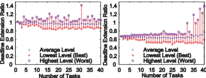
Fig. 3: Workload Prediction. (a) Lower Bound. (b) Upper Bound. We evaluate our designed algorithm with and without the prediction-error-tolerant support. That is, the system will test the Algorithm 1 with the tuned stricter deadline (D′) or the original one (D). We use Deadline Extension Ratio (DER)(defined as the ratio of task’s final execution time to its deadline) to evaluate the statistical task exe-cution lengths compared to their expected deadlines. We run 40 separate cases each with different number (1∼40) of tasks, and show the lowest/average/highest level of DER for each case.
Fig. 4: Deadline Extension Ratio (DER). (a)D′=D. (b)D′=α·D. We first show the experimental result by using the original deadline D (i.e., D′=D) in the algorithm. From Fig. 4 (a), we see that the tasks’ execution times cannot be always guaranteed to be executed within their deadlines in the worst case, no matter how many tasks (1∼40) are submitted. Specifically, even though the system avail-ability is relatively high (e.g., there are only several tasks submitted), the average value of deadline extension ratio is nearly to 1 and its highest value in the worst case is up to 1.2. This is mainly due to the inaccurate workload prediction with about 30% margin of errors as shown in Fig. 3. In comparison, Fig. 4 (b) shows the deadline extension ratio when the deadline D′ is set to a stricter deadline (α·D). When the number (denoted
by m) of tasks submitted scales up to 30, all tasks’ execution times can be kept nearly to about only 0.7 times as high as their preset deadlines (D) at the worst situation (i.e., the highest level shown in the figure). With further increasing number of the submitted tasks, tasks’ execution times cannot be always guaranteed because of the limited resource capacities (or the higher level of competitions on resources), but the mean level is still kept remarkably lower than 1, which means that most of the tasks can still meet the QoS (i.e., large majority can be finished before deadlines). Note that there are only 10 physical machines in our experiment but much more than 10 tasks can be processed with guaranteed deadlines, which indicates a remarkably high level on service consolidation. This also implies a great potential in improving resource utilization by taking advantage of VM-multiplexing feature.
0.1 0.2 0.3 0.4 0.5 0.6 0.7 0.8 0.9 1.0 1.2 1.3 1.4 Probability Distribution (Percentile of # of tasks)
Deadline Extension Ratio
Stricter-deadline-based Algorithm (D’=αD) Original-deadline-based Algorithm (D’=D) 0.35 0.525 0.225 0.175 0.125 1.1 0 0.2 0.4 0.6 0.8 1
Fig. 5: Distribution of DER (the number of Tasks)
Fig. 5 presents the distribution of the deadline ex-tension ratio (DER), in a competitive situation where there are 40tasks submitted. We observe that the stricter-deadline-based algorithm can more effectively limit the majority tasks’ execution times to about 0.7 times as high as the user-specified deadlines (i.e., the original ones), but it may suffer from higher DER at the worst case. In comparison, the majority of tasks (about 52.5%) un-der the original-deadline-based algorithm are completed within 0.95∼1.0 times of their deadlines, which still conforms to the deadline-guaranteed requirement; there are about 20% of tasks that would violate deadlines, most of which (17.5%) are still finished within 1.05 times of deadlines.
Finally, we evaluate the fairness of task processing in the two cases, confirming the stability. Based on Jain’s work [19], fairness index (higher value means higher fairness) is defined as Equation (24) whose value ranges in [0,1], wherexi refers to the DER of taskti.
F(x) =( ∑n
i=1xi)2
n∑n
i=1x2i (24)
We present the experimental results about the fairness index of the DER in Fig. 6. As observed, the fairness index is always kept over 0.99 for both cases under the relatively uncompetitive situation (e.g., m≤30), and still kept about 0.95 in the case with higher competition (i.e., whenm>30). Recall that there are only 10 physical machines used for resource provisioning in our exper-iment, which implies our solution’s allocation effect is
0.5 0.6 0.7 0.8 0.9 1 0 5 10 15 20 25 30 35 40 Fairness of DER Number of Tasks D’=αD D’=D
Fig. 6: Fairness Index of DER
confirmed to be quite stable to any task’s execution under such a dense server consolidation. In addition, the main reason for the degradation of the fairness of DER in the competitive situation is that the tasks with higher pri-orities or the ones arriving earlier would be treated with higher service level in our experiment, which would definitely impact other lower-priority tasks’ execution in the short-supply situation. In fact, guaranteeing the higher-priority tasks’s QoS by sacrificing lower-priority tasks’ benefit may also be considered a fairer treatment in many scenarios. Hence, for different applications, we can easily maximize the fairness level among all tasks by assigning the adaptive values for α, which will be further studied in our future work.
6
RELATED
WORK
Traditional job scheduling [20] is often formulated as a kind of combinatorial optimization problem (or queue-based multi-processor scheduling problem [21], [22], [12]), due to the non-guaranteed performance isolation for multiple tasks running on the same machines. That is, most of the existing deadline-driven task schedul-ing solutions (from sschedul-ingle cluster environment confined in LAN [23], [24] to the Grid computing environment suitable for WAN [25], [26]) are also strictly subject to the queueing model under which a single machine’s multiple resources cannot be further split to smaller frac-tions at will. This will eventually cause the raw-grained resource allocation, relatively low resource utilization and sub-optimal task execution efficiency.
With the VM resource isolation technology being ma-ture recently, it is viable to design more efficient re-source allocation due to the fledged performance iso-lation among VMs running on the same machines. X. Meng et al. [27] proposed a VM multiplexing based resource allocation approach, which can successfully analyze the compatibility of any two different VMs (each with an application running atop it) on the same physical machines, and reschedule the combination of the VMs to improve the overall performance. However, it cannot guarantee high compatibility among more than two VMs on the same machine. Q-Clouds [28] is another well-known system which can realize high consolidation of multiple VM-hosted applications, focusing on how to prevent inevitable performance interference among VMs from degrading user’s QoS or enhancing corresponding users’ payment unexpectedly.
Compared to the above existing works about VM-multiplexing resource allocation, our work aims to not only confine tasks’ execution to be within their dead-lines, but also minimize the payments for their users. This work will definitely benefit and motivate many Cloud users or service providers, who wish to minimize the infrastructure cost with the guaranteed QoS, actually already endeavored by many researchers. L. Wu et al. [29], for example, proposed a SLA-based resource allo-cation method, which is compatible to the heterogeneity of infrastructure and adaptable to the dynamic change of customer requests. It can maximize the profit of SaaS providers by minimizing the humber of SLA violations and the cost by reusing VMs. S. Chaisiri et al. [30] also aim to minimize the provisioning cost incurred to users by taking into account stochastic programming, robust optimization, and sample-average approximation together. M. Mao et al. [31], [32] present a Cloud auto-scaling mechanism to automatically scale computing instances based on workload information and perfor-mance desire, also aiming to guarantee task’s deadline with less payment. In comparison, our approach can be fundamentally proved optimal via the convex optimiza-tion theory, which we believe is a huge step forward especially from the perspective of theoretical analysis.
Most of the existing theoretical researches on Cloud computing [33], [34], [35] mainly focused on the rel-atively ideal scenarios by assuming tasks’ workloads can be accurately predicted, simplifying the resource allocation problem. For example, J. Weinman [33] an-alyzed the penalty functions working in the workload aggregation and relative statistical effects, given a set of fixed task workloads to be used, while V. Petrucci et al. [34] proposed an optimization VM-based model to minimize the power and management cost by as-suming that application’s consumption can be predicted precisely by monitoring system. Unlike these works, we theoretically analyze the upper bound of task’s execution time compared to its deadline and that of user-specified payment to the precise-prediction based result. By taking advantage of the derived bounds and approximation ratio, we can more effectively guarantee user tasks’ QoS in terms of their demands. To the best of our knowledge, this is the first attempt to study how to minimize the payment cost in the cloud system, which can also tolerate the prediction errors of tasks’ properties.
7
CONCLUSION AND
FUTURE
WORK
In this paper, we propose a novel resource alloca-tion algorithm for Cloud system that supports VM-multiplexing technology, aiming to minimize user’s pay-ment on his/her task and also endeavor to guarantee its execution deadline meanwhile. We can prove that the output of our algorithm is optimal based on the KKT condition, which means any other solutions would definitely cause larger payment cost. In addition, we ana-lyze the approximation ratio for the expanded execution
time generated by our algorithm to the user-expected deadline, under the possibly inaccurate task property prediction. When the resources provisioned are relatively sufficient, we can guarantee task’s execution time always within its deadline even under the wrong prediction about task’s workload characteristic. In the future, we plan to integrate our algorithms with stricter/orignal deadlines into some excellent management tools like OpenNebula, for maximizing the system-wide perfor-mance. Some queuing policies like earliest deadline first (EDF) will be studied to further reduce user payment especially in the short-supply situation. More complex scheduling constraints like the compatibility and security issue will also be taken into account.
ACKNOWLEDGMENTS
This research is supported by a Hong Kong RGC grant HKU 7179/09E and a Hong Kong UGC Special Equip-ment Grant (SEG HKU09).
REFERENCES
[1] M. Armbrust, A. Fox, R. Griffith, A. D. Joseph, R. H. Katz, A. Konwinski, G. Lee, D. A. Patterson, A. Rabkin, I. Stoica, and M. Zaharia, “Above the clouds: A berkeley view of cloud comput-ing,” EECS Department, University of California, Berkeley, Tech. Rep. UCB/EECS-2009-28, Feb 2009.
[2] L. M. Vaquero, L. Rodero-Merino, J. Caceres, and M. Lindner, “A break in the clouds: towards a cloud definition,”SIGCOMM Comput. Commun. Rev., vol. 39, no. 1, pp. 50–55, 2009.
[3] I. Foster and C. Kesselman, The Grid 2: Blueprint for a New Computing Infrastructure (The Morgan Kaufmann Series in Computer Architecture and Design). Morgan Kaufmann, November 2003. [4] J. E. Smith and R. Nair,Virtual Machines: Versatile Platforms For
Systems And Processes. Morgan Kaufmann, 2005.
[5] D. Gupta, L. Cherkasova, R. Gardner, and A. Vahdat, “Enforcing performance isolation across virtual machines in xen,” in Pro-ceedings of the ACM/IFIP/USENIX 2006 International Conference on Middleware (Middleware’06), New York, USA, 2006, pp. 342–362. [6] J. N. Matthews, W. Hu, M. Hapuarachchi, T. Deshane, D.
Di-matos, G. Hamilton, M. McCabe, and J. Owens, “Quantifying the performance isolation properties of virtualization systems,” inProceedings of the 2007 workshop on Experimental computer science (ExpCS ’07). New York, USA: ACM, 2007.
[7] Amazon elastic compute cloud: on line at http://aws.amazon.com/ec2/.
[8] D. Milojicic, I. M. Llorente, and R. S. Montero, “Opennebula: A cloud management tool,”Internet Computing, IEEE, vol. 15, no. 2, pp. 11 –14, march-april 2011.
[9] S. Boyd and L. Vandenberghe,Convex Optimization. Cambridge University Press, 2009.
[10] E. Imamagic, B. Radic, and D. Dobrenic, “An approach to grid scheduling by using condor-G matchmaking mechanism,” in28th International Conference on Information Technology Interfaces, 2006, pp. 625–632.
[11] B. Sharma, V. Chudnovsky, J. L. Hellerstein, R. Rifaat, and C. R. Das, “Modeling and synthesizing task placement constraints in google compute clusters,” inProceedings of the 2nd ACM Sympo-sium on Cloud Computing (SOCC’11). ACM, 2011, pp. 3:1–3:14. [12] H. Khazaei, J. V. Misic, and V. B. Misic, “Modelling of cloud
computing centers using m/g/m queues,” inICDCS Workshops, 2011, pp. 87–92.
[13] Y. Wu, K. Hwang, Y. Yuan, and W. Zheng, “Adaptive workload prediction of grid performance in confidence windows,” IEEE Transactions on Parallel and Distributed Systems, vol. 21, no. 7, pp. 925 –938, july 2010.
[14] S. Di, D. Kondo, W. Cirne,“Characterization and Comparison of Cloud versus Grid Workloads,” in Proceedings of 14th Interna-tional Conference on Cluster Computing (IEEE Cluster2012), 2012, pp. 230–238.
[15] Q. Zhang, , J. L. Hellerstein, and R. Boutaba, “Characterizing task usage shapes in google’s compute clusters,” inLarge Scale Distributed Systems and Middleware Workshop (LADIS’11), 2011. [16] L. Huang, J. Jia, B. Yu, B.G. Chun, P. Maniatis, and M. Naik,
“Predicting Execution Time of Computer Programs Using Sparse Polynomial Regression,” in24th Conference on Neural Information Processing Systems (NIPS’10). 2010, pp. 1–9.
[17] P. Barham, B. Dragovic, K. Fraser, S. Hand, T. Harris, A. Ho, R. Neugebauer, I. Pratt, and A. Warfield, “Xen and the art of virtualization,” inProceedings of the nineteenth ACM symposium on Operating systems principles (SOSP’03). New York, NY, USA: ACM, 2003, pp. 164–177.
[18] P. Wendykier and J. G. Nagy, “Parallel colt: A high-performance java library for scientific computing and image processing,”ACM Trans. Math. Softw., vol. 37, pp. 31:1–31:22, September 2010. [19] R. K. Jain, The Art of Computer Systems Performance Analysis:
Techniques for Experimental Design, Measurement, Simulation and Modelling. John Wiley & Sons, April 1991.
[20] C. Jiang, C. Wang, X. Liu, and Y. Zhao, “A survey of job schedul-ing in grids,” inProceedings of the joint 9th Asia-Pacific web and 8th international conference on web-age information management confer-ence on Advances in data and web management (APWeb/WAIM’07). 2007, pp. 419–427.
[21] P. Crescenzi and V. Kann,A compendium of NP optimization prob-lems. [Online]. Available: ftp://ftp.nada.kth.se/Theory/Viggo-Kann/compendium.pdf
[22] O. Sinnen, Task Scheduling for Parallel Systems (Wiley Series on Parallel and Distributed Computing). Wiley-Interscience, May 2007. [23] K. Ramamritham, J. A. Stankovic, and W. Zhao, “Distributed scheduling of tasks with deadlines and resource requirements.”
IEEE Trans. Computers, vol. 38, no. 8, pp. 1110–1123, 1989. [24] M. C. McElvany and P. D. Stotts, “Guaranteed task deadlines
for fault-tolerant workloads with conditional branches,”Real-Time Systems, vol. 3, no. 3, pp. 275–305, 1991.
[25] L. Zhao, Y. Ren, and K. Sakurai, “A resource minimizing schedul-ing algorithm with ensurschedul-ing the deadline and reliability in het-erogeneous systems,” in 25th IEEE International Conference on Advanced Information Networking and Applications (AINA’11), 2011, pp. 275–282.
[26] W. Chen, A. Fekete, and Y. C. Lee, “Exploiting deadline flexibility in grid workflow rescheduling,” in11th IEEE/ACM International Conference on Grid Computing (Grid’10), 2010, pp. 105–112. [27] X. Meng, C. Isci, J. Kephart, L. Zhang, E. Bouillet, and D.
Pen-darakis, “Efficient resource provisioning in compute clouds via vm multiplexing,” inProceeding of the 7th international conference on Autonomic computing (ICAC’10). ACM, 2010, pp. 11–20. [28] R. Nathuji, A. Kansal, and A. Ghaffarkhah, “Q-clouds :
Man-aging performance interference effects for qos-aware clouds,”
EuroSys2010, pp. 237–250, 2010.
[29] L. Wu, S. K. Garg, and R. Buyya, “Sla-based resource allocation for software as a service provider (saas) in cloud computing environments,” in 11th IEEE/ACM International Symposium on Cluster, Cloud and Grid Computing (CCGRID’11), 2011, pp. 195–204. [30] S. Chaisiri, R. Kaewpuang, B.-S. Lee, and D. Niyato, “Cost mini-mization for provisioning virtual servers in amazon elastic com-pute cloud,” in19th Annual IEEE/ACM International Symposium on Modeling, Analysis and Simulation of Computer and Telecommunica-tion Systems (MASCOTS’11), 2011, pp. 85–95.
[31] M. Mao, J. Li, and M. Humphrey, “Cloud auto-scaling with deadline and budget constraints,” in11th IEEE/ACM International Conference on Grid Computing (Grid’10), 2010, pp. 41–48.
[32] M. Mao and M. Humphrey, “Auto-Scaling to Minimize Cost and Meet Application Deadlines in Cloud Workflows,” inInternational Conference for High Performance Computing, Networking, Storage & Analysis (SC’11), 2011, pp. 49:1–49:12
[33] J. Weinman, “Smooth operator: The value of demand aggregation,” 2011. [Online]. Available: http://joeweinman.com/Resources/Joe Weinman Smooth Operator
Demand Aggregation.pdf
[34] V. Petrucci, O. Loques, and D. Moss´e, “A dynamic optimization model for power and performance management of virtualized clusters,” inProceedings of the 1st International Conference on Energy-Efficient Computing and Networking (e-Energy’10). New York, NY, USA: ACM, 2010, pp. 225–233.
[35] F. Chang, J. Ren, and R. Viswanathan, “Optimal resource alloca-tion in clouds,”IEEE International Conference on Cloud Computing, pp. 418–425, 2010.
Sheng Di Sheng Di received his M.Phil de-gree from Huazhong University of Science and Technology in 2007 and Ph.D degree from The University of Hong Kong in 2011. He is cur-rently a post-doctor researcher at INRIA. Dr. Di’s research interest involves optimization of distributed resource allocation especially in P2P systems and large-scale Cloud computing plat-forms. His background is mainly on the funda-mental theoretical analysis and practical system implementation. Contact him at the Department of Computer Science, The University of Hong Kong, Hong Kong, [email protected].
Cho-Li WangCho-Li Wang received his Ph.D. degree from University of Southern California in 1995. Dr. Wang’s research interests include multicore computing, software systems for Clus-ter and Grid computing, and virtualization tech-niques for Cloud computing. He serves on the editorial boards of several international jour-nals, including IEEE Transactions on Computers (2006-2010), Journal of Information Science and Engineering, and Multiagent and Grid Systems. He is the regional coordinator (Hong Kong) of IEEE Technical Committee on Scalable Computing (TCSC). Contact him at the Department of Computer Science, The University of Hong Kong, [email protected].