An Empirical Investigation of the Lucas Hypothesis: the Yield Curve and on Linearity in the Money-Output Relationship

An Empirical Investigation of the Lucas Hypothesis:

the Yield Curve and on Linearity in the Money-Output Relationship

Matteo Modena

University of Glasgow

First Draft: May 2009

This Draft: June 2010

Abstract

Existing evidence about the effectiveness of money growth to stimulate economic activity has been criticized from different perspectives. In addition, high correlation between money and output is not helpful to detect the direction of causality. From a policy perspective, in fact, positive correlation may arise from two opposite policy conducts: either the monetary authority sets the supply of money to influence future output fluctuations, or the central bank controls money growth as a reaction to the recent evolution of macro variables. In this work the relationship between money and output is analysed within a non linear framework that ascribes a primary role to expectations. In particular, we find evidence that the Lucas (1973) hypothesis, that exists an inverse correlation between the variance of nominal shocks and the magnitude of output response to nominal shocks, is supported by data evidence when the yield curve is either flat or downward sloping. We also provide evidence suggesting that the Friedman (1977) hypothesis, that the variability of inflation exerts a negative effect on the natural level of output, holds when a positive risk premium is incorporated in an upward sloping term structure of interest rates.

JEL classification: C01, C22, E32, E44, G12.

1. Introduction

Investigating the relationship between money and output has always been a major concern of macroeconomists. The classical dichotomy about whether money influences the future level of output or, viceversa, whether output fluctuations influence money supply, is still an unresolved puzzle. Economists affiliated to the monetarist school believe that money growth will be merely reflected in the future price level, at least this is assumed to be true over long horizons. However, the monetarist view that money does not affect real output may be a weak argument in the short run. On the other hand, Keynesian economists think that short run policies may well influence the level of economic activity.

In this contribution we would like to investigate whether there is a direct relationship between money, or a measure of it, and output; alternatively, we examine whether the effect of money on the business cycle is contingent to other factors, such as, for instance, the shape of the yield curve. We analyse the relationship between money and output within a non linear empirical framework that allows for rational expectations. In particular, we investigate whether the Lucas (1973) hypothesis, that there is a negative relationship between the variance of nominal shocks and the magnitude of output response to nominal shocks, is supported by data evidence. The contrarian argument, that the conditional variance of money forecast errors negatively affects the natural level of output, has been proposed by Friedman (1977).

Working with US post-war data, we find evidence that conditioning the examination of the money-output relation to the shape of the yield curve gives the opportunity of reconciling the aforementioned opposite views1

. Evidence seems to suggest that the variability of inflation, captured by the conditional variance of money forecast errors, exerts a negative influence on output when the yield curve is upward sloping. There is also some evidence that the Friedman hypothesis holds when the linear model is estimated over the entire sample (from 1967 to 2007).

However, in the regime characterized by a flat or downward sloping yield curve the Lucas hypothesis seems to prevail. Interpreting the variance of nominal shocks as agents’ perception of monetary policy uncertainty, there seems to be an inverse correlation between aggregate uncertainty and output response. Aggregate risk displays greater effect the more agents internalize uncertainty. In that agents’ actions are driven by a large amount of precaution resulting in mild output changes. We thus provide evidence supporting the Lucas hypothesis which is usually rejected by data in linear analysis (Kim and Nelson, 1989).

The weaknesses of traditional models (King and Plosser, 1984; Ravn and Sola, 2004) coupled with the difficulty of detecting a unique direction for causality call for an approach that emphasizes the role of expectations. Hence, the contribution of this study is also methodological. We propose to examine expectations exploiting a two-level structure: micro and macro.

At a micro level (bottom level) agents’ expectations focus on the central bank operational procedure regarding the supply of money. The micro mechanism of processing available informationisbased on the Kalmanfilter which implies acontinuous refinement of expectations on the basis of past prediction errors, i.e. deviations between ex ante expected and ex post observed values of the money stock. In such a setting agents form expectations according to a Bayesian iterative sequence that combines the re-elaboration of past prediction errors with the analysis of new flows of information. Moreover, what is peculiar in the micro analysis of expectations is that Kalman filtering allows separating the expected from the unexpected component of money growth. The adoption of a time-varying approach for the policy rule is also consistent with recent evidence. Cogley and Sargent (2006), as well as Boivin (2006), document important time variation in the response of the monetary authority to the state of the economy. Also Sims and Zha (2006) point out that the changing view of the Fed about the economy has been gradual; they argue it could be attributed to the changes of shocks’ variance. Finally, Primiceri (2008) provides evidence that the reaction of monetary policy to the changes in both inflation and unemployment has become more and more aggressive in the last decades. Last, but certainly not least, we focus on a policy rule expressed in terms of money supply since our sample is characterized by periods of inflation instability; Bernanke and Mishkin (1993) argue, in fact, that central banks tend to adopt targets in terms of money growth when the inflation rate threatens to be out of control.

At a macro level (top level) expectations focus on the future economic outlook, as reflected by the dynamics of the term structure of interest rates. The macro perspective captures the sentiment regarding the future evolution of key macro variables as well as institutional or socio-political factors, or, eventually, technological changes. There is in fact large evidence that the information content of term structure could be used to make inference about the future state of the economy (Estrella and Hardouvelis, 1991; Estrella and Mishkin, 1997). Several studies point out that she slope of the yield curve help forecasting output fluctuations; more recent evidence focuses on the predictive role of term premia implied by the term structure (Hamilton and Kim, 2002; Favero, Kaminska, and Soderstrom, 2005; Ang, Piazzesi, and Wei, 2006; Rudebusch, Sack, and Swanson, 2008; Modena, 2008 a). Finally, Modena (2008 b, 2011) draws attention to the fact that also curvature, and not only extreme points of the yield curve, may be related to output movements.

Furthermore, our methodology partially accounts for the criticism moved by Amato and Swanson (2000). Despite some evidence suggests monetary aggregates help predict future output (Stock and Watson, 1989; Becketti and Morris, 1992; Feldstein and Stock, 1994), Amato and Swanson point out that such evidence might be contingent upon the nature of the dataset. Using real time, rather than revised, data they document a substantial reduction of the marginal predictive power of money. The threshold approach adopted in this work implies non linearity in the dataset thus breaking time continuity; for this reason specifically, it allows reducing the impact of the historical track.

The rest of the paper is organized as follows. The next Section contains a brief survey of the literature and discusses motivations. In Section 3 we present some evidence about causality. In Section4 we outline the structure of expectations at the micro level. Empirical evidence is discussed in Section 5. Finally, Section6 concludes. Data are presented in Appendix I. In Appendix II we report auxiliary estimations.

2. Motivations and Literature Review

Whether and to what extent money growth is capable of contributing to the determination of real output is still an unresolved puzzle in economics. The monetarist view that money growth induces a proportional change in the price level leaving real output unaffected is acknowledged to work in the medium-long run. However, as Keynesian theory suggests, monetary disturbances are believed to have some real effects in the short run. Although the contribution of monetary shocks on permanent income growth is limited or absent, managing money supply is a useful instrument under control of the central bank for stabilizing or stimulating the economy across the business cycle.

The classical dichotomy of money neutrality, i.e. nominal variables are unable to affect real variables, has been initially investigated by means of the following equation, which is known as the Saint Louis equation since it has been introduced by economists of that Federal Reserve District:

t t t t t t t t t t t M M M M trend IP =α +β ∆ +β ∆ +β ∆ +β ∆ +β +ε ∆ _{,−3 0 ,−3 1 −3,−6 2 −6,−9 3 −9,−12 4} (1) The LHS variable is the quarterly change in the industrial production index; while, the quarterly changes of the money stock over the last year are explanatory variables. The above regression also includes a constant and a time trend (to account for eventual trend in money and output growth). Different monetary aggregates have been considered: M1, M2, and the U.S. Fed Board of Governors monetary base (MB). The analysis is performed on monthly data from 1967 to 2007. Empirical results are reported in Table 1.

.

Saint Louis Equation - IP grw (3)

α β₀ β₁ β₂ β₃ β₄ R2 M1 1.2986 -0.1155 0.1551 0.0822 0.0686 0.0013 0.027 t-stat (0.1318) (0.0963) (0.0312) (0.2534) (0.3221) (0.5490) NW (0.5261) (0.2251) (0.1359) (0.4039) (0.4407) (0.7734) W (0.2081) (0.1465) (0.0504) (0.2466) (0.2651) (0.5728) M2 -0.0020 -0.1238 0.1447 0.1191 0.0593 0.0005 0.094 t-stat (0.0710) (0.0016) (0.0007) (0.0051) (0.1292) (0.0262) NW (0.4226) (0.0069) (0.0027) (0.0361) (0.2146) (0.2781) W (0.1166) (0.0007) (0.0001) (0.0062) (0.1138) (0.0364) MB -0.0093 0.4487 0.5870 0.3514 0.3628 0.0001 0.019 t-stat (0.4713) (0.2062) (0.1004) (0.3263) (0.3101) (0.3757) NW (0.7033) (0.3348) (0.1775) (0.3638) (0.4721) (0.6656) W (0.4594) (0.1458) (0.0428) (0.1478) (0.2115) (0.3926)

p-values in parenthesis. NW: Newey-West correction. W: White correction.

IP grw (3): 3-month growth of the seasonally adjusted industrial production index

(dependent variable). Regressors appear in the equation as quarterly rate of growth:

M1: monetary aggregate M1; M2: monetary aggregate M2; MB: monetary base.

.

Table 1

The contemporaneous effect on output exerted by M2 turns out to be negative (β₀< 0); however, more generally, results suggest that the rate of growth of M2 over the last three quarters have a positive influence on IP growth (β₁,β₂> 0). The rate of growth of M1 has a marginal, though significant, effect on the current growth of the IP index.

In order to check whether there is a significant influence of money on output we have looked at the jointly significance of estimated coefficients in each equation. In all the equations, coefficients turn out to be jointly significant supporting the influence of money on output. In addition, we have also run a Wald test to check the following restrictions:

∑

= =

3

0 0

i βi , i.e. to check whether money growth

does explain output. The null hypothesis is rejected in two cases since the probability value associated to the test is zero for both M2 and MB equations, thus suggesting the influence of these monetary aggregates on real activity. M1 growth, instead, does not seem informative about output. As a forecasting exercise we have estimated the above regression using the future determination of output in the LHS: t t t t t t t t t t t M M M M trend IP =α+β ∆ +β ∆ +β ∆ +β ∆ +β +ε ∆ _{+3, 0 ,−3 1 −3,−6 2 −6,−9 3 −9,−12 4} (2) Results reported in Table 2 suggest that M2, rather than M1 and the monetary base, is effective in influencing both the current and the future level of industrial production. In the equation for M2 both coefficients β₀ and β₁ are statistically significant indicating that future output is influenced by

money growth up to six months before. The goodness of fit is definitely poor; however, the M2 equation returns a much better fit than the other equations. The dynamics of M1 over the most recent quarter has a marginal impact on the IP growth.

. St. Louis Equation - IP grw (+3) α β₀ β₁ β₂ β₃ β₄ R2 M1 0.0228 0.0304 0.0190 0.0215 -0.0181 0.0005 0.025 t-stat (0.2877) (0.0796) (0.2883) (0.2321) (0.2941) (0.3033) NW (0.6378) (0.2752) (0.4457) (0.2973) (0.4842) (0.6076) W (0.3499) (0.0812) (0.2828) (0.1945) (0.2622) (0.3162) M2 -0.0074 0.2269 0.2916 0.0989 -0.0191 0.0001 0.075 t-stat (0.0101) (0.0223) (0.0068) (0.3563) (0.8461) (0.0081) NW (0.2359) (0.1031) (0.0492) (0.4050) (0.8891) (0.1906) W (0.0197) (0.0126) (0.0101) (0.3488) (0.8458) (0.0112) MB -0.0011 0.1584 0.1056 0.1041 0.0086 0.0004 0.017 t-stat (0.7192) (0.0771) (0.2396) (0.2474) (0.9238) (0.4298) NW (0.8391) (0.1954) (0.2347) (0.3739) (0.9369) (0.6890) W (0.6976) (0.0422) (0.0674) (0.1437) (0.9073) (0.4349)

p-values in parenthesis. NW: Newey-West correction. W: White correction.

IP grw (+3): quarterly growth of the seasonally adjusted industrial production index

over the next 3-month period (dependent variable). Regressors appear in the equation as quarterly rate of growth: M1: monetary aggregate M1; M2: monetary aggregate M2; MB: monetary base.

.

Table 2

The macroeconomic debate has further focused on the asymmetric effect of monetary policy on output. Models with sticky prices or financial constraints suggest that interest rate changes generate greater effect on real activity during recessions. Similarly to Romer and Romer (1994), Garcia and Schaller (1999) find evidence in line with this conjecture arguing that monetary policy is more effective during recessions. Ravn and Sola (2004) find evidence corroborating the hybrid traditional Keynesian asymmetry, that is only small negative monetary policy shocks tend to influence real output. In order to account for this effect we estimate the above equations including dummy variables to distinguish the effect of positive rather than negative money growth rates.

t t t t t t t t t t t D M D M D M D M IP =

α

+

β

∆ +

β

∆ +

β

∆ +

β

∆ +

ε

∆ + _{− −} − − + − − + − + − 9, 12 ) ( 3 9 , 6 ) ( 2 6 , 3 ) ( 1 3 , ) ( 0 3 , (3) t t t t t t t t t t t D M D M D M D M IP =

α

+

β

∆ +

β

∆ +

β

∆ +

β

∆ +

ε

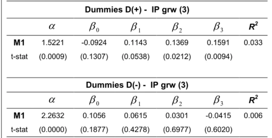
∆ − _{− −} − − − − − − − − − 9, 12 ) ( 3 9 , 6 ) ( 2 6 , 3 ) ( 1 3 , ) ( 0 3 , (4)

Where D(+) indicates a positive quarterly growth rate of the monetary aggregate, while D(-) indicates a negative growth rate. Results strongly support the hypothesis advanced by Romer and Romer (1994). Coefficients are statistically significant only in equation (3), as reported in the top panel of

Table 3, suggesting that only stimulus to economic activity seem to be effective. Moreover, the goodness of fit (0.033) of equation (3) is much larger than that (0.006) of equation (4) -bottom panel of Table 3-. The F-test suggests coefficients are jointly significant only in equation (3). The Wald test confirms that the null hypothesis

∑

= =

3

0 0

i βi cannot be rejected for equation (3) solely.

. Dummies D(+) - IP grw (3) α β₀ β₁ β₂ β₃ R2 M1 1.5221 -0.0924 0.1143 0.1369 0.1591 0.033 t-stat (0.0009) (0.1307) (0.0538) (0.0212) (0.0094) Dummies D(-) - IP grw (3) α β₀ β₁ β₂ β₃ R2 M1 2.2632 0.1056 0.0615 0.0301 -0.0415 0.006 t-stat (0.0000) (0.1877) (0.4278) (0.6977) (0.6020) p-values in parenthesis.

IP grw (3): 3-month growth of the seasonally adjusted industrial production

index (dependent variable). Regressors appear in the equation as quarterly rate of growth: M1: monetary aggregate M1; D(+): dummy variables that capture positive changes of the quarterly growth of the monetary aggregate;

D(-): dummy variables that capture negative changes of the quarterly growth of the monetary aggregate.

.

Table 3

Results are similar when replacing the dependent variable ∆IP_t,t−3 with its future realization ∆IP_t+3,t: . Dummies D(+) - IP grw (+3) α β₀ β₁ β₂ β₃ R2 M1 0.3606 0.0352 0.0335 0.0323 -0.0157 0.032 t-stat (0.0019) (0.0220) (0.0247) (0.0301) (0.3046) Dummies D(-) - IP grw (+3) α β₀ β₁ β₂ β₃ R2 M1 0.5663 0.0910 0.0747 -0.0459 0.0242 0.005 t-stat (0.0000) (0.6507) (0.7008) (0.8131) (0.2246) p-values in parenthesis.

IP grw (+3): quarterly growth of the seasonally adjusted industrial

production index over the next 3-month period (dependent variable). Regressors appear in the equation as quarterly rate of growth: M1: monetary aggregate M1; D(+): dummy variables that capture positive changes of the quarterly growth of the monetary aggregate; D(-): dummy variables that capture negative changes of the quarterly growth of the monetary aggregate.

.

Table 4

Although not reported, and coherently with the estimations above, the joint estimation of an equation including all dummy variables, both D(+) and D(-), returns significant coefficients only for dummies D(+)denoting an increase of the monetary aggregate.

The main drawback of the above equations is that they are not sufficient to establish any causality relation running from money to output. King and Plosser (1984) observe that monetary aggregates such as M1 and M2 are determined by the interaction between the high-powered money, a liability of the central bank, the behaviour of both firms and households, and the efficiency of the financial system through the strategies of the banking sector. Therefore it is possible to observe changes in the money stock that anticipate output movements without causing them.

Endogeneity is the second problem associated with both equations (1) and (2) and equations (3) and (4). The high correlation eventually captured by the coefficients of the equations may well derive from the conduct of the monetary authority that sets the future supply of money in response to past output fluctuations. The chronological sequence of a tight monetary policy which follows growing GDP, like a reduction of the rate of money growth whose final goal is to curb economic activity, and of an accommodative policy to tackle falling GDP preserves high correlation between money and output but with important implications for reverse causation. In addition, from a policy point of view, it is impossible to ascribe to monetary policy the effect of money on output without simultaneously considering the effect on GDP exerted by fiscal policies. The poor good of fit obtained for the above regressions is, in fact, a sign of misspecification; in particular, some relevant variables may be omitted.

Finally, the time series analysis performed by estimating the above equations might be affected by shifts in money demand since financial innovations contributes to changing agents’ preferences. In particular, as Ravn and Sola (2004) argue, the instability of M1 demand may underlie the poor fit of the M1 equation; furthermore, and specifically in this analysis, the monthly frequency of data may, in principle, accentuate the effect of M1 volatility.

The aforementioned intrinsic difficulties of detecting the effect of money on output coupled with the devastating effect of the Lucas critique call for an empirical method based on dynamic expectations as that implied by Kalman filtering. Expectations are subject to continuous refinement as long as new information becomes available; in addition, agents revisit their expectations on the base of past prediction errors. So far, in fact, we have not discriminated between anticipated and unanticipated money growth which is a core distinction in economics. In this vein, prediction errors work like a proxy for unanticipated money supply. Our approach will be deeply motivated later. Before presenting in details the methodology adopted in this chapter, next Section provides some more evidence regarding the money-output relation.

3. Preliminary Evidence on Causality

In this Section we focus on the causality issue characterizing the empirical relationship between real variables and monetary aggregates. Using monthly data from January 1967 to December 2007, we start by looking at dynamic short-run correlations. Each panel of Figure 1 shows correlations between a measure of real activity and different monetary aggregates (M1, M2, and MB, the monetary base). The top-left diagram indicates that all monetary aggregates are positively correlated with the Hodrick-Prescott detrended series of industrial production at lags, but negatively correlated at leads. Hence, booms (high IP relative to trend) tend to be preceded by high values of money growth; while positive values of IP relative to its HP trend tend to be followed by low values of money growth. This evidence is in line with the idea that money supply acts as a stimulus to real economic activity; while in response to fast-growing economy, and to the associated threat of mounting inflation, the monetary authority inverts the sign of the monetary policy conduct. The bottom-left diagram shows the correlations between monetary aggregates and the annual change in the unemployment rate. Consistently with the above story, all monetary aggregates are negatively correlated at lags with the growth in unemployment, i.e. a reduction in unemployment tends to be preceded by high values of money supply; on the other hand, monetary aggregates are positively correlated with the increase of unemployment at leads.

-.4 -.2 .0 .2 .4 M1 grw M2 grw MB grw IP gap (HP) -24 -20 -16 -12 -8 -4 0 4 8 12 16 20 24 -.4 -.2 .0 .2 .4 M1 grw M2 grw MB grw real CONS grw -24 -20 -16 -12 -8 -4 0 4 8 12 16 20 24 IP gap (HP): industrial production gap obtained with the Hodrick-Prescot filter.

real CONS grw: annual

growth of the seasonally adjusted real personal consumption expenditures.

M1 grw: annual growth of

monetary aggregate M1. M2 grw: annual growth of monetary aggregate M2. MB grw: annual growth of the monetary base. -.4 -.2 .0 .2 .4 M1 grw M2 grw MB grw UN grw -24 -20 -16 -12 -8 -4 0 4 8 12 16 20 24 -.4 -.2 .0 .2 .4 M1 grw M2 grw MB grw TCU (ln) -24 -20 -16 -12 -8 -4 0 4 8 12 16 20 24 UN grw: annual growth of

the unemployment rate. TCU (ln): log total capacity utiliation. M1 grw: annual growth of monetary aggregate M1. M2 grw: annual growth of monetary aggregate M2. MB grw: annual growth of the monetary base.

Figure 1

The top-right diagram of Figure 1 shows the pattern of short run correlations between the change in real consumption expenditures and monetary aggregates. Private consumption seems to be

positively related to money growth in the short run at both leads and lags. The smoother pattern of the monetary base correlations is consistent with the theory put forward by King and Plosser (1984); they find that inside money, i.e. the internal monetary measures which represent the liabilities of the banking sector as a component of monetary aggregates, rather than outside money, i.e. the external monetary measures which represent the liabilities of the central bank, are positively correlated with real activity.

Finally, although lower with respect to other real indicators, the bottom-right panel shows that the correlation between monetary aggregates and the (log) total capacity utilization is positive at both lags and leads; thus both past money supply and expectations of future important money supply tend to positively affect the employment of the factors of production.

Previous evidence is provided by Friedman and Schwartz (1963) in a classical contribution about the monetary history of the United States; they find that money growth rate changes lead changes in real GDP. The left diagram of Figure 2 shows that the rate of growth of M1 systematically anticipates business cycle movements between 1967 and the mid 1980s. Falling money growth precedes slowdowns in economic activity; while increasing money stocks anticipate both recoveries and booms. However, more recent evidence presented in the right diagram is more controversial: starting from 1985, in fact, the relationship between money and output is not as close as before, both the length and the magnitude of cyclical fluctuations do not reproduce the preceding dynamics of the monetary aggregate. The different pattern of the relationship between M1 and the IP gap might be due to financial innovations which affected the demand for money. The greater variability of the rate of growth of M1 might also reflect greater difficulty of the money stock to influence output from 1986 and 1997. In addition, Choudhry (2002) finds that the stated monetary act of 1980 considerably affected the income and interest rate demand elasticities of both M1, M2 and their components in U.S. Moreover, he argues that the fall in the M1 interest rate elasticity may well indicate M1 as possibly a more effective monetary policy tool after 1980.

68 70 72 74 76 78 80 82 84 86 M1 grw IP gap (HP) 88 90 92 94 96 98 00 02 04 06 M1 grw IP gap (HP) M1 grw: annual growth of monetary aggregate M1. IP gap (HP): industrial production gap obtained with the Hodrick-Prescot filter.

In line with the above evidence, the following scatter diagrams suggest a stronger effect displayed on both current and future output (detrended IP) by M2 rather than by M1 or MB2

. The top diagrams show the scatter between the IP gap and the contemporaneous growth rate of the monetary aggregates. In the bottom panels we report the scatter plots between the actual HP-detrended IP and the rate of money growth 12 months before.

-.15 -.10 -.05 .00 .05 .10 .15 -.10 -.05 .00 .05 .10 .15 .20 M1 grw IP g a p ( H P ) -.15 -.10 -.05 .00 .05 .10 .15 -.10 -.05 .00 .05 .10 .15 .20 M2 grw IP g a p ( H P ) -.15 -.10 -.05 .00 .05 .10 .15 -.10 -.05 .00 .05 .10 .15 .20 MB grw IP g a p ( H P ) -.15 -.10 -.05 .00 .05 .10 .15 -.10 -.05 .00 .05 .10 .15 .20 M1 grw (-12) IP g a p ( H P ) -.15 -.10 -.05 .00 .05 .10 .15 -.10 -.05 .00 .05 .10 .15 .20 M2 grw (-12) IP g a p ( H P ) -.15 -.10 -.05 .00 .05 .10 .15 -.10 -.05 .00 .05 .10 .15 .20 MB grw (-12) IP g a p ( H P )

Scatter plot diagrams. IP gap (HP): industrial production gap obtained with the Hodrick-Prescot filter. M1 grw: annual growth of monetary aggregate M1. M2 grw: annual growth of monetary aggregate M2. MB grw: annual growth of the monetary base. (-12) means the twelfth lag (monthly frequency of data).

Figure 3

As Walsh (2003) points out “while suggestive, evidence based on time patterns and simple correlations may not indicate the true casual role of money. Since the Federal Reserve and the banking sector respond to economic developments, movements in the monetary aggregates are not exogenous, and the correlation patterns need not reflect any casual effect of monetary policy on economic activity”. Notwithstanding the above mentioned stronger influence on real variables exerted by M2 than other aggregates, the Granger causality tests suggest M1 being the only source capable of affecting the future level of both industrial production and total capacity utilization. The null hypothesis that the rate of growth of M1 does not cause the IP gap cannot be rejected, as well as the null that M1 does not cause (log) TCU. The real personal consumption expenditure seems to be caused in the Granger sense by all monetary aggregates. Results are reported in Table 5.

2

The regressing line associated to M2 is, in fact, always steeper. The only exception occurs in the mid-bottom panel, the regressing line associated to MB turns out to be marginally steeper than the one associated to M2. However, in the former case (MB) there is a greater vertical dispersion of observations around the regressing line; in the latter case (M2), instead, observations more closely

.

Granger Causality Test

lags IP gap (HP) TCU (log) unemp r-cons

M1 3 (0.0432) (0.0296) (0.8090) (0.3827) 6 (0.0577) (0.0158) (0.8598) (0.0063) 12 (0.7340) (0.6834) (0.1455) (0.0066) M2 3 (0.1971) (0.1568) (0.6825) (0.0013) 6 (0.2398) (0.4621) (0.2978) (0.0005) 12 (0.4150) (0.2986) (0.1740) (0.0050) MB 3 (0.5173) (0.5698) (0.7667) (0.0321) 6 (0.7928) (0.9175) (0.7430) (0.1002) 12 (0.2935) (0.2558) (0.3408) (0.0436) Null Hypothesis: the monetary aggregate does not Granger-cause the real variable. Tests p-values in parenthesis.

IP gap (HP): industrial production gap obtained with the Hodrick-Prescott filter;

TCU (log): log-series of the total capacity utilization; unemp: unemployment

rate; r-cons: real personal consumption expenditures. M1: monetary aggregate M1; M2: monetary aggregate M2; MB: monetary base.

.

Table 5

The Granger tests are also employed to investigate whether lagged levels of the real variables help to predict the future path of monetary aggregates. Results are significantly supportive in this respect, as shown in Table 6. Such statistical evidence about causality is compatible with a Taylor-type monetary policy reaction function implying the monetary authority to raise the policy rate when the pace of economic growth is as fast as to create undesired inflationary pressures.

.

Granger Causality Test

lags M1 M2 MB IP gap (HP) 3 (0.0002) (0.0003) (0.0765) 6 (0.0231) (0.0003) (0.0239) 12 (0.0914) (0.0004) (0.1145) unemp 3 (0.0100) (0.0002) (0.1510) 6 (0.0408) (0.0006) (0.3795) 12 (0.0606) (0.0136) (0.4834) TCU 3 (0.0055) (0.0170) (0.4816) 6 (0.0321) (0.0053) (0.0407) 12 (0.1117) (0.0136) (0.1669) r-cons 3 (0.0046) (0.0005) (0.0778) 6 (0.1192) (0.0008) (0.1646) 12 (0.3280) (0.0340) (0.6395) Null Hypothesis: the real variable does not Granger-cause the monetary aggregate. Tests p-values in parenthesis.

M1: monetary aggregate M1; M2: monetary aggregate M2; MB: monetary base. IP gap (HP): industrial production gap obtained with the Hodrick-Prescott filter; TCU (log): log-series of the total capacity utilization; unemp: unemployment rate; r-cons: real personal consumption expenditures.

.

We sum up the preliminary evidence discussed in this Section by saying that results regarding the effect of money on output turn out to be somehow ambiguous. Short run correlations tend to suggest a positive influence of lagged money on actual output; however, the Granger tests partially contradict this evidence by suggesting a causality relationship working in the opposite direction. In addition, despite the existing evidence suggesting that money helps to predict future output (Stock and Watson, 1989; Becketti and Morris, 1992; Feldstein and Stock, 1994), Amato and Swanson (2000) argue that results are someway misleading because they crucially depends on revised, rather than real time, monetary aggregates data.

The aforementioned ambiguity can be dealt with by introducing a new element in the analysis; we thus attribute a role of primary importance to agents’ expectations and, in particular, to the associated expectations errors. To conclude, we recall that the choice of M1 as the benchmark reference aggregate for the monetary policy rule in the following analysis hinges on the results of the Granger tests reported in Table 5.

4. Empirical Methods for Expectations

In this Section we summarize the approach employed to derive agents’ expectations about the future stance of monetary policy as captured by the rate of growth of M1.

King and Plosser (1984), in fact, suggest inside money, a component of M1 representing the liabilities of the banking sector, being highly correlated with business cycle movements. In addition, Bernanke and Mishkin (1993) argue that the monetary authority tends to define targets in terms of money growth if there is a concrete likelihood that inflation gets out of control. Our sample is characterized by periods of high and volatile inflation. Finally, we justify the time-varying approach by observing that there is substantial evidence highlighting that both the monetary policy conduct and the variance of nominal shocks have changed over time (Cogley and Sargent, 2006; Boivin, 2006; Sims and Zha, 2006; Primiceri 2008).

We thus compute expectations by applying the Kalman filter, since it provides with an effective formalisation of the mechanism through which agents form expectations rationally. Moreover, the Kalman approach gives the opportunity of deriving a measure of innovations which overcomes the criticism traditionally moved to the VAR approach. In what follows we briefly outline the main features of Kalman filtering.

The observation equation, or measurement equation, of the state-space system is:

t t t t a x u M = + + ∆ ₋1β (5)

Actual quarterly money growth is a function of the changes of the T-bill rate, of the price level, and of the money stock over the previous quarter; u_t is a stochastic i.i.d.

(

0,σ_u

)

noise. The specification of the money equation come from Mishkin (1982) and Weintraub (1980); it has been successively considered by Kim and Nelson (1989). The only difference is that we rule out the fiscal variable, because of the superior independence achieved by the monetary authority in recent times. The state, or transition, equation captures the evolution of coefficients over time:

t t

t =µ +F β−1+v

β (6)

Where v_t is an idiosyncratic disturbance i.i.d.

(

0,σ_v

)

. Following standard practice, we impose matrix F to be the identity matrix since we assume that the regressing coefficients follow random walk processes (Kim and Nelson, 1998; Kim and Nelson, 2006; Boivin, 2006). The Kalman filter is an iterative algorithm based on updating the informative set with most recent available information and predicting future movements of the variable under examination. The coefficients covariance matrix conditional on information available up to time t-1 is:

(

)(

)

[

I

]

t t t t t t t t E P|−1 = β −β |−1 β −β|−1 (7)

Equation (8) provides the predictionof money growth based on information available up to time t

given that economists know the econometric relationship linking the core variable to the explanatory variables till time t-1.

1 | 1

|− = −

∆M_tt x_tβ_tt (8) Once the actual contemporaneous value of the core variable is observed, agents can compute the prediction error according to the following

1 ! 1 | 1 |t− =∆ t − t tt− =∆ t −∆ tt− t M x β M M η (9) Finally, equation (10) represents the conditional variance of money growth prediction errors:

[ ]

2 1 | 2 1 | 1 |− =

η

− = − +

σ

ε I t t t t t t t t E xP x h (10)

According to (10) Kalman filtering allows two sources of uncertainty generating the conditional variance of the forecast error (h ). One source depends on the evolutionary behaviour of

estimated coefficients through the coefficients covariance matrix, thus capturing the gradual change of the policy regime over time; the other source is a random noise related to future disturbances, like unpredictable institutional or technological shocks. The assumption of a constant variance of nominal shocks to money growth seems too severe since aggregate M1 is regarded to respond on a great variety of shocks. First, M1 trivially depends upon the monetary policy conduct through the money supply (high-powered money). Second, M1 is affected by the interaction between money supply and money demand, so that a demand shock, rather than a supply shock, may influence aggregate M1. For instance financial innovations as well as deregulation may affect M1 in the medium-short run. Finally, M1 depends also on the strategic decisions of the banking system and on the credit market conditions. Therefore, a measure of variance which is conditional to the state of the economy provides with a more realistic picture of aggregate risk.

An alternative method to compute the time-varying conditional variance is to estimate an autoregressive model for money growth (either AR or VAR, depending on the nature of the analysis), and then to compute the squared of fitted residuals3

(Piazzesi, 2003).

5. Empirical Results

In this Section we provide evidence that the Lucas hypothesis, i.e. that exists a negative relationship between the variance of nominal shocks and the magnitude of output response to nominal shocks, usually rejected in linear model, holds when the likelihood of a slowdown in economic activity is warned by financial indicators. Evidence also suggests that the alternative Friedman hypothesis, that the augmenting variability of inflation exerts a negative effect on output, tends to hold when financial indicators anticipate a thriving pace of economic growth.

A crucial issue involved in testing the Lucas hypothesis is the examination of the conditional variance of nominal shocks over time. Hence, the analysis starts with the estimation of time-varying monetary policy function expressed in terms of money rather than in terms of the rate of interest. The inverse relationship tying money supply and interest rates is trivially respected in any modern economy; moreover, the extensive sample period covered in this analysis calls for a generic version of the monetary policy rule.

After estimating a time-varying specification of equations (5) and (6), we obtain a series of prediction errors (η_t|t−1) and a measure of forecast errors’ conditional volatility (h_t|t−1). The basic equation to test the Lucas versus the Friedman hypothesis is the following:

3

t t t t t t t h gap v gap =α0 +α1η|₋1 +α2 |₋1+α3 ₋1+ (11)

Where the output gap is the HP de-trended series of log IP. In addition, coefficient

α

₁ is set equal to

1 | 1 0

1 =γ +γ htt−

α . The functional form of

α

₁ is motivated with the aim of reducing the effect of multi-collinearity in the OLS regression. Equation (11) thus becomes

(

tt tt

)

tt t t t

t

t h h gap v

gap =α₀ +γ₀η_|−1 +γ₁η_|−1⋅ _|−1 +α_{2 |−1}+α_{3 −1}+ (11’)

The inclusion of the first lag of the dependent variable, which is highly correlated with its actual level, certifies the robustness of other coefficients estimates. In addition, different computational methods for the variance-covariance matrix have been employed in order to obtain consistent estimates (White, 1980; Hansen and Hodrick, 1980; Newey and West, 1987; and, finally, the simplified Hansen and Hodrick).

The theory advanced by Lucas is satisfied when both

γ

₀ >0 and

γ

₁ <0; while, testing the Friedman hypothesis is equivalent to detecting whether coefficient

α

₂ is negative (

α

₂ <0)4. The assumption here is that the conditional variance of money forecast errors acts as a proxy for the variability of inflation. The original idea put forward by Friedman (1977), in fact, is that the variability of inflation, rather than that of money, reduces the natural level of output since it disturbs the allocation efficiency of the price system.

The linear model (11’), estimated over the entire sample 1967-2007, does not reveal any particular information about the way nominal shocks affect business cycle fluctuations. Table 7 shows estimation results for different measures of the business conditions. The dependent variable in the top panel is the Hodrick-Prescott measure of the IP gap; (from the top to the bottom) in the second panel the dependent variable is the log total capacity utilization; in the third panel the dependent variable is the rate of unemployment; finally, in the bottom panel, the dependent variable is the rate of change of unemployment5

.

There is weak evidence supporting the Friedman hypothesis. Although coefficient

α

₂ is inversely related to the dynamics of real variables, it is either marginally or not significant with the only exception holding for unemployment. The Lucas hypothesis is definitely rejected. Coefficient

γ

₀ is

4

not statistically significant. In two cases coefficient

γ

₁ turns out to be significantly positive thus contradicting the Lucas hypothesis6

. .

joint estimation - IP gap (HP)

0

α

γ

₀

γ

₁

α

₂

α

3 R 2 OLS -0.1198 0.0436 -0.0158 -0.0182 0.9444 0.906 t-stat [-1.423] [1.238] [-1.143] [-1.544] [64.75] W [-1.346] [1.485] [-1.325] [-1.410] [54.71] obs 468 HH (12) [-1.501] [1.884] [-1.552] [-1.702] [95.31] NW (12) [-1.342] [1.634] [-1.449] [-1.531] [55.74] s-HH [-0.656] [1.474] [-1.181] [-0.812] [22.92] . .

joint estimation - TCU

0

α

γ

0

γ

1

α

2

α

3 R 2 OLS -0.9839 0.0163 0.0283 -0.0003 0.9780 0.974 t-stat [2.893] [0.958] [2.181] [-0.846] [127] W [-2.816] [0.971] [2.107] [-1.123] [124] obs 468 HH (12) [-1.894] [0.880] [2.409] [-1.835] [83.27] NW (12) [-1.839] [0.873] [2.291] [-1.360] [80.98] s-HH [-0.918] [1.267] [1.174] [-0.848] [40.26] . .

joint estimation - Unemployment

0

α

γ

₀

γ

₁

α

2

α

3 R 2 OLS -0.2986 -0.1251 0.0012 0.0077 0.9870 0.985 t-stat [-0.805] [-0.301] [0.522] [2.458] [173] W [-0.771] [-0.298] [0.786] [2.895] [149] obs 468 HH (12) [-0.472] [-0.462] [0.973] [2.991] [83.63] NW (12) [-0.501] [-0.339] [0.881] [3.005] [88.19] s-HH [-0.257] [-0.398] [0.555] [1.323] [53.01] . .

joint estimation - Unemployment grw

0

α

γ

₀

γ

₁

α

₂

α

3 R 2 OLS 0.1502 -0.0852 0.0861 0.0102 0.9634 0.933 t-stat [0.027] [-0.867] [1.710] [0.134] [76.10] W [0.027] [-0.812] [2.189] [0.137] [59.75] obs 468 HH (12) [0.031] [-1.700] [5.122] [0.208] [89.14] NW (12) [0.027] [-0.968] [2.819] [0.158] [49.62] s-HH [0.013] [-1.139] [1.719] [0.075] [25.62] t-statistics in square brackets.

OLS: ordinary least squares estimation; W: White correction; HH: Hansen Hodrick correction; NW: Newey-West correction; s-HH: simplified Hansen-Hodrick correction (see Cochrane and Piazzesi, AER 2005).

.

Table 7

The linear estimation of equation (11’) is not entirely reliable though, since the pattern of residuals series is affected by heteroscedaticity in all cases. In addition, a strong ARCH effect is found after

6

In AppendixII we report the estimation of equation (11’) using an alternative measure of the conditional variance of money growth forecast errors leading to similar results. In particular, after estimating an unrestricted VAR (9) model of money growth, inflation, and the change in the 3-month T-bill rate, we obtain the conditional variance of money forecast errors as the squares of residuals

performing the Engle (1982) test. The recursive residuals and the CUSUM square of residuals reveal the instability of coefficient estimates as reported in Figure 47

. Finally, also the Hansen tests (1992, 2000) highlight the presence of non-linearity.

-3 -2 -1 0 1 2 3 4

recursive resid std err

-0.2 0.0 0.2 0.4 0.6 0.8 1.0 1.2 CUSUM sqr 5% significance Figure 4

Therefore, we consider a non linear version of model (11’) allowing for two different regimes determined by slope of the term structure, i.e. the difference between the 10-year and the 3-month yields8

. The slope of the yield curve is believed to reflect agents’ expectations about the future stance of monetary policy and, thus, it is thought to anticipate business cycle movements (Estrella and Hardouvelis, 1991; Estrella and Mishkin, 1997). Conditioning the test of the Lucas hypothesis to the slope of the term structure means to relating agent’s expectations to a leading economic indicator (Stock and Watson, 1989). In particular, the yield curve represents a link between monetary policy, the financial sector and the real economy. We recall that the peculiar aspect of this methodology is to consider expectations on a double level. At the first level, the micro level, expectations are modelled through Kalman filtering the money supply function in order to isolate prediction errors (Section 4). At the second level, the macro level, expectations have a

forward-looking nature in that they are intended to capture the future evolution of the economy as reflected

by the dynamics of the term structure of interest rates. Macro expectations interpret a perspective sentiment present throughout the economy, a broad view regarding the economic conditions, including political as well as institutional, or technological, factors.

A crucial issues to be pointed out is that the micro level analysis of expectations is performed on a monetary policy function expressed in terms of money supply. While, the macro level expectations are inferred by the evolution of the yield curve, whose dynamics depends not only on the determination of the policy rate, or a measure closely related to it as it may be the effective federal funds rate, but also on the abovementioned factors. The choice of the monetary policy function in terms of the money stock is thus intended to separate two different levels of expectations’ analysis.

We aim at distinguishing the expectations regarding the operational procedure of the monetary authority in setting the money supply from the overall movements displayed by the yield curve. Although there exists an unquestionable inverse relationship linking money supply and short rates, the evolution of the yield curve, as well as the determination of expectations at a macro level, depend on a greater variety of factors. So that we believe our approach is immune from the criticism that the micro and macro structures for expectations share a common root9

.

The threshold methodology implies that the same equation is estimated in two different regimes depending on the values assumed by a predetermined variable (

τ

), i.e. the yield spread which is a measure of the slope of the term structure.

(

)

(

)

     > + + + ⋅ + + = ≤ + + + ⋅ + + = − − − − − − − − − − τ τ α α η γ η γ α τ τ α α η γ η γ α ˆ ˆ 1 3 1 | 2 1 | 1 | 1 1 | 0 0 1 3 1 | 2 1 | 1 | 1 1 | 0 0 if v gap h h gap if v gap h h gap t t t t t t t t t t t t t t t t t t t t t t (12)

Regime 1 is determined by values of the yield spread below the estimated threshold (τˆ ); hence, the first regime is characterized by a flat or downward sloping yield curve. The conventional view tends to associate such a regime to an imminent slowdown in economic activity. On the other hand, regime 2 is defined on high values of the spread (positive slope of the yield curve) reflecting an accommodative stance of monetary policy. Estrella and Hardouvelis (1991), as well as Estrella and Mishkin (1997), present important evidence that the yield spread is related to the future evolution of real activity. In particular, a downward sloping or a flat yield curve augments the odds of a recession in the near future. Along the same line Wright (2006) finds a link between the shape of the yield curve and the probability of future economic slowdowns.

Estimation results for regime 1 (below the estimated threshold) are show in Table 8. The Lucas hypothesis seems to be respected regardless the variable used to measure the business cycle. The conditional variance of money growth affects real variables through the coefficients of the prediction-error term (

γ

₁). The direct influence of the conditional variance implied by the Friedman hypothesis is not significant with the only exception for the IP gap equation, where surprisingly the effect of the conditional variance appears to work in the opposite direction. However, this is far from being paradoxical as long as when the economy is going toward a recession, a peak in the variability of inflation, captured by the conditional variance of money growth, might act as a stimulus to economic activity, or might be interpreted as a sign that the recession is neither severe nor long-lasting.

9

. REGIME 1 - IP gap (HP) 0

α

γ

₀

γ

₁

α

₂

α

₃ R2 OLS 0.4327 0.0291 -0.0118 0.0080 0.9039 0.860 t-stat [1.603] [1.524] [-1.809] [2.246] [19.60] W [2.083] [2.245] [-1.893] [2.358] [21.60] obs 74 HH (12) [2.857] [2.644] [-1.838] [5.067] [19.49] NW (12) [2.222] [2.004] [-1.693] [2.533] [18.95] s-HH [0.912] [1.975] [-1.557] [1.630] [12.74] . . REGIME 1 – TCU 0

α

γ

₀

γ

₁

α

₂

α

3 R 2 OLS -0.6857 0.0242 -0.0119 0.0017 0.9844 0.968 t-stat [-1.584] [2.651] [-2.632] [0.971] [100] W [-1.531] [2.373] [-2.188] [1.017] [97.12] obs 355 HH (12) [-1.474] [2.134] [-1.993] [1.448] [93.61] NW (12) [-1.463] [2.256] [-2.080] [1.194] [92.99] s-HH [-0.809] [2.928] [-2.967] [0.777] [51.40] . . REGIME 1 – unemployment 0

α

γ

0

γ

1

α

2

α

3 R 2 OLS 0.2949 -0.0472 0.0232 -0.0063 0.9967 0.985 t-stat [0.071] [-2.188] [2.177] [-1.547] [146] W [0.073] [-1.914] [1.790] [-1.611] [145] obs 362 HH (12) [0.081] [-1.761] [1.708] [-1.842] [129] NW (12) [0.084] [-1.875] [1.812] [-1.692] [143] s-HH [0.033] [-2.399] [2.409] [-1.356] [70.28] . . REGIME 1 - unemployment grw 0

α

γ

₀

γ

₁

α

₂

α

3 R 2 OLS -0.1966 -0.0126 0.0622 0.0174 1.0198 0.913 t-stat [-2.558] [-2.175] [2.148] [1.553] [47.98] W [-2.615] [-2.551] [2.484] [1.566] [43.52] obs 248 HH (12) [-6.869] [-2.325] [2.147] [4.158] [37.65] NW (12) [-3.198] [-2.257] [2.189] [1.843] [43.36] s-HH [-1.532] [-2.305] [2.357] [1.217] [39.38] t-statistics in square brackets.

OLS: ordinary least squares estimation; W: White correction; HH: Hansen Hodrick correction; NW: Newey-West correction; s-HH: simplified Hansen-Hodrick correction (see Cochrane and Piazzesi, AER 2005).

.

Table 8

Generated variables in the above regression might invalidate inference procedures. To handle with it not only we propose alternative measures of the standard errors (White, 1980; Hansen and Hodrick, 1980; Newey and West, 1987; the simplified Hansen and Hodrick), but also we perform a Monte Carlo simulation. Results show a clear convergence of both Lucas parameters towards the true values just after few thousands replications (

γ

₀ in the left panel;

γ

₁ in the right panel). The top diagrams show the simulation with 15000 replications, while in the bottom diagrams we run 50000

.010 .015 .020 .025 .030 2500 5000 7500 10000 12500 15000

MC simul std err true coef.

-.014 -.012 -.010 -.008 -.006 -.004 -.002 2500 5000 7500 10000 12500 15000

MC simul std err true coef.

.016 .020 .024 .028 .032 10000 20000 30000 40000 50000

MC simul std err true coef.

-.014 -.012 -.010 -.008 -.006 -.004 10000 20000 30000 40000 50000

MC simul std err true coef.

Figure 5

The estimation of regime 1 has also been performed after ruling out the conditional variance of money prediction errors. Results are reported in Table 9. There is a clear confirmation that the Lucas hypothesis is not rejected by the data when the yield curve is either flat or downward sloping.

. REGIME 1 - IP gap (HP) 0

α

γ

₀

γ

₁

α

₂

α

3 R 2 OLS 0.0414 0.0245 -0.0123 0.9554 0.843 t-stat [1.152] [2.963] [-3.007] [58.41] W [1.143] [2.599] [-2.449] [49.35] obs 74 NW (12) [1.143] [2.438] [-2.279] [50.81] . . REGIME 1 – TCU 0

α

γ

₀

γ

₁

α

₂

α

3 R 2 OLS -0.5250 0.0254 -0.0125 0.9878 0.968 t-stat [-1.261] [2.852] [-2.861] [104] W [-1.183] [2.529] [-2.342] [98.19] obs 355 NW (12) [-1.126] [2.391] [-2.207] [93.54] .

t-statistics in square brackets.

OLS: ordinary least squares estimation; W: White correction; NW: Newey-West correction.

REGIME 1 – Unemployment 0

α

γ

0

γ

1

α

2

α

3 R 2 OLS -0.1997 -0.0532 0.0265 0.9998 0.985 t-stat [-0.513] [-2.503] [2.525] [153] W [-0.535] [-2.243] [2.124] [147] obs 362 NW (12) [-0.557] [-2.151] [2.124] [152] . . REGIME 1 - Unemployment grw 0

α

γ

₀

γ

₁

α

₂

α

₃ R2 OLS -0.0843 -0.0179 0.0522 1.0085 0.911 t-stat [-3.209] [-1.891] [1.841] [50.35] W [-3.237] [-1.941] [1.833] [45.45] obs 248 NW (12) [-3.298] [-1.872] [1.778] [45.00]

t-statistics in square brackets.

OLS: ordinary least squares estimation; W: White correction; NW: Newey-West correction.

.

Table 9 (b)

Before showing results for the second regime we would like to offer an insight about the above results. When the variance of nominal shocks tends to be relatively high, it is also true that the actions of the monetary authority are governed by a considerable amount of uncertainty, since predictions errors are quite volatile. Thus, if the central bank cannot easily recognize which is the most suitable strategy to be implemented given the current economic scenario, economic agents internalize such insecurity and assume more balanced and measured behaviors, for instance consumers stop spending money on superfluous goods, and firms refrain from investing in capital goods. Aggregate actions result in output responses that are mild, i.e. of lower magnitude. Hence, there is an inverse relationship between variance of nominal shocks and the magnitude of business cycle fluctuations. This relationship is also true when the variance of nominal shocks tends to be relative small. Suppose the yield curve is flat due to severe monetary policy correctly expected by agents (again this case perfectly fits regime 1), in such an atmosphere output would react heavily falling below the steady state level thus preserving the inverse correlation highlighted by Lucas (1973).

Regime 2 is characterized by high, and positive, values of the yield spread. Regime 2 estimates are reported in Table 10.

. REGIME 2 - IP gap (HP) 0

α

γ

₀

γ

₁

α

₂

α

₃ R2 OLS -0.2375 0.0059 0.0009 -0.0371 0.9436 0.904 t-stat [-2.683] [0.170] [0.064] [-2.949] [57.55] W [-2.902] [0.220] [0.096] [-3.213] [48.44] obs 394 HH (12) [-2.731] [0.214] [0.090] [-3.033] [62.92] NW (12) [-2.685] [0.194] [0.082] [-3.045] [52.57] s-HH [-1.558] [0.136] [0.054] [-2.332] [39.26] . . REGIME 2 - TCU 0

α

γ

₀

γ

₁

α

₂

α

3 R 2 OLS 0.4740 0.0351 -0.0076 -0.0041 1.012 0.982 t-stat [0.787] [0.815] [-0.480] [-2.502] [73.79] W [0.690] [1.023] [-0.694] [-3.385] [64.84] obs 113 HH (12) [1.948] [1.039] [-0.814] [-4.501] [181] NW (12) [0.911] [1.044] [-0.711] [-3.227] [85.78] s-HH [0.930] [0.603] [-0.363] [-2.308] [86.72] . . REGIME 2 – Unemployment 0

α

γ

0

γ

1

α

2

α

3 R 2 OLS 0.3876 -0.0263 0.0131 0.0096 0.9874 0.938 t-stat [0.394] [-0.223] [0.301] [2.114] [77.32] W [0.246] [-0.249] [0.412] [3.314] [46.66] obs 106 HH (12) [0.476] [-0.237] [0.439] [5.850] [63.61] NW (12) [0.325] [-0.214] [0.381] [4.067] [50.27] s-HH [0.452] [-0.157] [0.217] [1.904] [95.88] . . REGIME 2 - Unemployment grw 0

α

γ

₀

γ

₁

α

₂

α

3 R 2 OLS 0.1910 -0.0211 0.0983 0.0169 0.9416 0.953 t-stat [2.664] [-0.842] [1.026] [1.745] [63.27] W [2.906] [-0.780] [1.119] [2.050] [51.02] obs 220 HH (12) [6.212] [-0.752] [1.164] [4.223] [39.94] NW (12) [3.392] [-0.767] [1.165] [2.377] [45.15] s-HH [1.618] [-0.627] [0.803] [1.468] [58.52] t-statistics in square brackets.

OLS: ordinary least squares estimation; W: White correction; HH: Hansen Hodrick correction; NW: Newey-West correction; s-HH: simplified Hansen-Hodrick correction (see Cochrane and Piazzesi, AER 2005).

.

Table 10

The monetary accommodation reflected in the upward sloping term structure is usually expected to stimulate economic activity thus pushing the economy on an expansionary path. On the other hand, a positive slope of the yield curve implies a positive risk premium required by investors to move to longer horizons. In particular, Ang, Bekaert and Wei (2008) find evidence that the slope of the nominal term structure is due to a positive inflation risk premium. In case of perfect foresight about future spot rates, in fact, the arbitrage mechanism would equalize holding period returns along the entire spectrum of maturities implying a flat yield curve. In a context characterized by imperfect

information, uncertainty causes the term structure to deviate from its risk-neutral implied shape. The joint effect of uncertainty and economic growth is reflected in a greater variability of expected inflation, and, thus, in the dynamics of the conditional variance of money growth (Barro, 1976; Friedman, 1977). Therefore, the threshold estimation of regime 2 should return a significant coefficient

α

₂ stressing out the inverse relationship between the money conditional variance and the economic cycle. Coefficient

α

₂ is, in fact, negative in the equations expressed in terms of the IP gap and the total capacity utilization; while, coefficient

α

₂ turns out to be positive when the dependent variable is unemployment or its rate of change. As Rudebusch, Sack and Swanson (2007) have found, this result can be interpreted in the sense that there exists an inverse correlation between term premia and output growth.

6. Concluding Remarks

In this work we propose and implement an innovative method for expectations in order to investigate the relationship between money and output. Previous evidence tends to support the view that money is effective in stimulating real economic activity; however, some contrarian evidence suggests the issue is still controversial. In particular, the high correlation between money and output does not reveal an unambiguous direction of causality. From a policy perspective, in fact, the aforementioned positive correlation can derive from two opposite phenomena. On the one hand, the monetary authority can govern the supply of money to influence the future economic conjuncture; on the other hand, the central bank can manage the dynamics of monetary aggregates in response of past macroeconomic conditions. In addition, the weaknesses associated to traditional approaches call for an effective role of expectations.

After estimating a time-varying monetary policy rule where expectations are analysed at a micro

level, we condition the examination of the money-output relationship to the shape of the yield curve. In particular, in this paper we test the Lucas (1973) hypothesis against Friedman’s (1977). Within a non linear approach, we find evidence that the conditional variance of money growth affects real output through the coefficients on the forecast error term in the Lucas-type output equation only when the flat shape of the term structure reflects expectations of a slowdown in economic activity. Moreover, the conditional variance of money growth, which is used as a proxy for inflation variability, appears to affect directly output, thus corroborating Friedman’s theory, when the term structure is upward sloping, i.e. investors require a positive term premium.

References

Amato J. D., Swanson . R., 2000, The Real-Time Predictive Content of Money for Output, Bank for International Settlements, Woking Paper.

Andrews D.W.K., 1993, Tests for Parameter Instability and Structural Change with Unknown Change Point,

Econometrica, Vol. 55.

Ang A., Bekaert G., Wei M., 2008, The Term Structure of Real Rates and Expected Inflation, Journal of Finance, Vol. 63.

Ang A., Piazzesi M., 2003, A 1o-Arbitrage Vector Autoregression of Term Structure Dynamics with Macroeconomic

and Latent Variables, Journal of Monetary Economics, Vol. 50.

Ang A., Piazzesi M., Wei M., 2006, What Does the Yield Curve Tell Us about GDP Growth?, Journal of Econometrics, Vol. 131.

Barro R. J., 1976, Rational Expectations and the Role of Monetary Policy,Journal of Monetary Economics, Vol. 2.

Becketti S., Morris C., 1992, Does Money Matter Anymore? A Comment on Friedman and Kuttner, Working Paper Fed of Kansas City.

Bekaert G., Hodrick R. J., 2001, Expectations Hypothesis Tests, Journal of Finance, Vol. 56.

Bekaert G., Cho S., Moreno A., 2005, 1ew-Keynesian Macroeconomics and the Term Structure of Interest Rates, NBER Working Paper.

Bernanke B. S., Blinder A.S., 1992, The Federal Funds Rate and the Channel of Monetary Transmission, American Economic Review, Vol. 82.

Bernanke B. S., Mishkin F., 1993, Central Bank Behaviour and the Strategy of Monetary Policy: Observations from

six Industrialized Countries, NBER Working Paper.

Bernanke B. S., Mihov I., 1998, Measuring Monetary Policy, The Quarterly Journal of Economics, Vol. 113.

Boivin J., 2006, Has U.S. Monetary Policy Changed? Evidence from Drifting Coefficients and Real Time Data,

Journal of Money, Credit and Banking, Vol. 38.

Campbell J. Y., 1995, Some Lessons from the Yield Curve, Journal of Economic Perspectives, Vol. 9.

Campbell J.Y., Cochrane J.H., 1999, By Force of Habit: a Consumption-Based Explanation of Aggregate Stock

Market Behaviour, Journal of Political Economy, Vol. 107.

Campbell J.Y., Lo A.W., MacKinlay A.C., 1997, The Econometrics of Financial Markets, Princeton University Press.

Campbell J. Y., Shiller R. J., 1987, Cointegration and Tests of Present Value Models, Journal of Political Economy, Vol. 95.

Campbell J.Y., Shiller R.J., 1991, Yield Spreads and Interest Rate Movements: A Bird’s Eye View, Review of Economic Studies, Vol. 58.

Cerrato M., Kim H., MacDonald R., 2008, 3-Regime Symmetric STAR Modelling and Exchange Rate Reversion. University of Glasgow Working Paper.

Chapman D.A., 1997, The Cyclical Properties of Consumption Growth and the Real Term Structure, Journal of Monetary Economics, Vol. 39.

Choudhry T., 2002, Financial Innovations and Demand for United States M1 and M2 Components, International Economic Journal, Vol. 16.

Cochrane J.H., 1999, 1ew Facts in Finance, Economic Perspectives XXIII, Fed of Chicago.

Cochrane J.H., 2005, Asset Pricing, Princeton University Press.

Cochrane J.H. Piazzesi M., 2005, Bond Risk Premia, American Economic Review, Vol. 95.

Cogley T., Sargent T., 2005, Drift and Volatilities: Monetary Policies and Outcomes in the Post WWII U.S., Review of Economic Dynamics, Vol. 8.

Engle R.F., 1982, Autoregressive Conditional Heteroscedasticity with Estimates of the Variance of United Kingdom

Inflation, Econometrica, Vol. 50.

Estrella A., 2004, Why Does the Yield Curve Predict Output and Inflation?, Economic Journal, Royal Economic Society, Vol. 115.

Estrella A., Hardouvelis G.A., 1991, The Term Structure as a Predictor of Real Economic Activity, Journal of Finance, Vol. 46.

Estrella A., Mishkin F.S., 1999, Predicting U.S. Recessions: Financial Variables as Leading Indicators, NBER Working Papers.

Estrella A., Mishkin F.S., 1997, The Predictive Power of the Term Structure of Interest Rates in Europe and the

United States: Implications for the European Central Bank, European Economic Review, Vol. 41.

Evans C.L., Kuttner K. ., 1998, Can VARs Describe Monetary Policy?, Working Paper Fed of Chicago.

Evans C.L., Marshall D.A., 2007, Economic Determinants of the 1ominal Treasury Yield Curve, Journal of Monetary Economics, Vol. 54.

Fama E.F., 1984, The Information in the Term Structure, Journal of Financial Economics, Vol. 13.

Fama E.F., 1984, Term Premium in Bonds Returns, Journal of Financial Economics, Vol. 13.

Favero C.A.,2006, Taylor Rule