Pooling risk among countries

Pooling risk among countries

LSE Research Online URL for this paper:

http://eprints.lse.ac.uk/102909/

Version: Accepted Version

Article:

Callen, Mike, Imbs, Jean and Mauro, Paolo (2015) Pooling risk among countries.

Journal of International Economics, 96 (1). pp. 88-99. ISSN 0022-1996

https://doi.org/10.1016/j.jinteco.2015.01.006

[email protected]

Reuse

Items deposited in LSE Research Online are protected by copyright, with all rights

reserved unless indicated otherwise. They may be downloaded and/or printed for private study, or other acts as permitted by national copyright laws. The publisher or other rights holders may allow further reproduction and re-use of the full text version. This is

Pooling Risk Among Countries

∗

Michael Callen

Jean Imbs

Paolo Mauro

December 2014

Abstract

Suppose that international sharing risk—worldwide or with large num-bers of countries—were costly. How much risk-sharing could be gained in small sets (or “pools”) of countries? To answer this question, we com-pute the means and variances of poolwide gross domestic product growth, for all possible pools of any size drawn from a sample of 74 countries, and compare them with the means and variances of consumption growth in each country individually. From the difference, we infer potential di-versification and welfare gains. As much as two-thirds of the first best, full worldwide welfare gains can be obtained in groupings of as few as seven countries. The largest potential gains arise from pools consisting of countries in different regions and including countries with weak insti-tutions. We argue international risk-sharing fails to emerge because the largest potential gains are among countries that do not trust each other’s willingness and ability to abide by international contractual obligations.

Keywords: Risk Sharing, Diversification. JEL Classification: E21, E32, E34, F41.

∗_{We are grateful to two anonymous referees, and to Eric van Wincoop, Tamim Bayoumi,} Mick Devereux, Michael Kremer, Raghuram Rajan, Jaume Ventura, and seminar participants at U.C. Berkeley, Cambridge U., the International Monetary Fund, U. Pompeu Fabra, the San Francisco Fed, and Tufts U. for insightful suggestions; to Nicolas Metzger, and Jos´e Romero for superb research assistance; and to Jean Salvati and especially Huigang Chen and Alin Mirastean for invaluable help in programming and computational support. Financial support from the Banque de France Chair at the Paris School of Economics is gratefully acknowledged. All errors are our own. Corresponding author: Jean Imbs - Paris School of Economics - 106 Bvd de l’Hopital - 75013 Paris, France. [email protected].

†_{Kennedy School of Government, Harvard University} ‡_{Paris School of Economics (CNRS) and CEPR.} §_{Peterson Institute for International Economics}

1

Introduction

Despite major strides in lifting capital controls around the world and impressive increases in cross-border holdings of financial assets, international financial in-tegration is still far from complete: Individual countries’ consumption remains more volatile than what would result from complete risk-sharing with the rest of the world. In this paper, we conjecture that practical obstacles make inter-national risk sharing costly, and that they depend on the number and charac-teristics of potential partner countries to share risk with. Then, it can become

desirable to share risk within a well chosen subset of countries only.1 _{This paper}

evaluates the potential gains associated with such limited risk sharing contracts. How large would such groups need to be for the gains to be sizable? And which groups would yield the largest gains?

Our main contribution consists in running a systematic search on all possi-ble groupings, or “pools” of countries, using the variance-covariance matrix of output and consumption growth rates observed in standard data for 74 coun-tries. We compare the observed volatility of consumption for each country with

the volatility of poolwide output, for each possible pool.2 _{Consumption data}

are relevant because they reflect the insurance mechanisms that already exist in each country. Under risk sharing within the pool, consumption growth in each country equals poolwide output growth. Therefore, the comparison quan-tifies the potential for additional diversification gains—and ultimately welfare gains—that would accrue to each country from moving to complete risk-sharing within each pool considered. For any possible pool size, we identify the country groupings that minimize poolwide GDP volatility, and maximize welfare gains from international diversification.

We find that pools of fewer than ten countries can provide the bulk of the potential first best, worldwide risk sharing gains. In those well chosen groupings,

1

We do not observe worldwide risk sharing, but we do not observe sharing of GDP risk within groups of countries either. How could risk sharing be achieved in practice for a subset of countries? Various schemes have been proposed, including Robert C. Merton’s (1990, 2000) networks of bilateral swaps of GDP-linked income streams. Elements of risk sharing among groups of countries are also present, for example, in pooling arrangements for international reserves, such as the Chiang Mai initiative, the Latin American Reserve Fund (FLAR), or networks of bilateral swap arrangements (e.g., among the G7 in the 1960s-70s, among the European countries during the run up to the establishment of the Euro, and among several countries during the global financial and economic crisis that began in 2007-8). While these existing real-world arrangements do not seek to share GDP risk explicitly, they do imply some degree of sharing of macroeconomic risks among their member countries. On FLAR, see Eichengreen (2007) and www.flar.net; on the Chiang Mai initiative, see Park and Wang (2005), and http://aric.adb.org; on the earlier European experience, see Eichengreen and Wyplosz (1993). On the sharing of GDP risks more generally see Shiller (1993); and Borensztein and Mauro (2004) for a review of the literature.

2

In this regard, our approach differs from previous studies: by Obstfeld (1994) and Lewis (2000), who used consumption data only, and by Tesar (1995), who modeled explicitly the saving / investment decisions that determine production in general equilibrium. However, the paper’s results are unchanged if we use consumption data only, or production data only.

the marginal gains decline quickly for groups beyond six or seven members. Many small pools yield large risk-sharing gains. Unsurprisingly, such pools

involve relatively volatile economies.3

If the gains from international risk sharing are so significant, and could in principle be attained in relatively small groups of countries, why do such arrangements not emerge more often? One possibility is that they face partic-ularly costly obstacles. As we show in the paper, the largest potential gains are often attained by sharing risk with distant countries characterized by weak institutional quality and a history of default on international debt obligations. In that light, the observed reluctance to engage in international risk-sharing becomes less surprising: it may just stem from insufficient information about the trustworthiness of potential partners or difficulties related to international law. Then, risk sharing is especially costly precisely in those small groups of countries where they would carry maximal gains.

To explore this issue further, we report the potential gains that would result from risk-sharing arrangements if they were constrained to countries selected from a universe with certain characteristics—the same geographic region, or relatively strong institutions. In those potential country groupings, the costs associated with sharing GDP risk are presumably lower, and so a local arrange-ment is more likely to emerge. But as we show, these are also countries whose GDP risks tend to be strongly correlated, and so where the gains from risk sharing are smaller in the first place.

The rest of the paper is organized as follows. Section II provides the theo-retical background to our empirical exercise— adapted from existing work. The section also outlines how we handle the considerable combinatorial problem in-volved in manipulating a sample of 74 countries. Section III presents the general results on risk-sharing gains across subsets of countries. In Section IV, we esti-mate how much risk sharing gains are reduced when countries are constrained to share risk only with specific partners. Section V concludes.

2

Methodology

This section first outlines the theory motivating the paper’s empirics. Then it describes the algorithms used to compute the risk sharing gains, in any subset of countries, of any size, drawn from a universe of 74 countries with available consumption and output data.

3

Pallage and Robe (2003) show that the welfare cost of economic fluctuations is far larger in developing countries than in advanced economies.

2.1

Risk-Sharing, Volatility, and Welfare

The argument relies on a well known framework, based on Lewis (2000) and Obstfeld (1994). As they do, we abstract from non tradability and non separa-bility in utility, and from the possible impact of uncertainty on growth. These simplifications enable us to compute the welfare gains for risk sharing among a

large set of 74 countries.4

Following Epstein and Zin (1989), utility at timetin countryj is given by

Utj= ( Ctj 1−θ +β Et Utj+1 1−γ(1−θ)(1−γ) )1/(1−θ) (1)

where Ctj is consumption at time t in country j. The process for endowment

income at timetin countryj is

yjt =y j t−1+µj− 1 2σ 2 j+ε j t (2) where yjt = lnY j t and ε j t ∼ N 0, σj2

. 0 < β < 1 denotes the subjective

discount rate, γ > 0 is the coefficient of relative risk aversion and θ is the

inverse of the elasticity of intertemporal substitution in consumption.µjdenotes

the long run growth rate of output in country j, and σ2

j its variance around

trend growth. Equation (2) assumes permanent shocks to income, which is well known to magnify the welfare gains from diversification, for any pool size. But the assumption does not affect how quickly welfare gains increase with the number of countries sharing risk, the paper’s main question. The assumption of permanent shocks is maintained for tractability.

As in Lewis (2000), the analysis focuses on the welfare gains afforded by inter-national diversification. This assumes away alternative sources of consumption smoothing, such as self insurance and saving. It is consistent with the purpose

of evaluating the potential from international risk sharing. Following Lewis

(2000)Ctj=Y

j

t under autarky, and timet welfare in countryj is given by

Utj =C j t 1−βMj1−θ −1/(1−θ) (3) whereMj = exp µj−1₂γσj2

. If instead countryj enters a risk sharing

agree-ment, it will have a claim on poolwide income, ¯Yt, which we assume is distributed

log-normally, with mean ¯µand volatility ¯σ2_{: ¯y}

t= ¯yt−1+ ¯µ−21σ¯2+ ¯εt.5 In the

pool, timetwelfare in countryj is therefore given by

¯ Utj = ¯C j t 1−βM¯1−θ −1/(1−θ) (4) 4

With non-separabilities, the literature usually considers two countries only, see Cole and Obstfeld (1991) or Coeurdacier (2009). Lewis and Liu (2014) consider up to eight countries, but have to deal with issues of existence and uniqueness.

5

Lewis (2000) shows the sum of log-linear processes can be approximated by a log-linear process.

where ¯M = exp ¯µ−1₂γσ¯2

, and ¯Ctj is consumption in country j at time t if

the country is part of the risk sharing pool.

How much of a claim does countryjhave on poolwide output? The only asset

available in countryjis the security that paysYtj, whose price is denoted byp

j t.

Entering the pool means acquiring the security that pays poolwide output ¯Yt,

whose price is denoted by ¯pt. Therefore, as in Lewis (2000) country j’s claim

on poolwide output at timet >0 is given by

¯ Ctj= pjt ¯ pt ¯ Yt (5)

We now introduce the possibility that a cost has to be paid by any countryj

willing to participate in the risk sharing agreement. The cost τj is paid once

and for all, at the time the agreement is contracted: it could for instance be paid outside of the pool, to a supra-national agency, whose remit is to monitor the agreement is subsequently honored, or to help provide relevant information

about the pool’s members.6 _{If the risk sharing agreement is contracted at time}

0, this implies ¯ C₀j =p j 0−τj ¯ p0 Y0¯ (6)

The cost τj affects only the level of initial consumption in country j, at the

time the pool is contracted: In particular, it does not affect the subsequent growth rates of consumption for all countries in the pool. They are all equal

to the growth in ¯Yt.7 Therefore the introduction of the cost τj does not alter

the dynamic properties of the equilibrium established in Lewis (2000), which we now discuss.

Once it is in the pool, consumption in country j obeys the following Euler

equation for allt >0:

1 =βφEt  R¯ φ−1 t+1R j t+1 ¯ Ctj+1 ¯ Ctj !−θφ  (7) withφ= γ−1 θ−1, ¯Rt+1= ¯ Yt+1+ ¯pt+1 ¯ pt , andR j t+1= Ytj+1+p j t+1 pj_t+1 . Analogously, poolwide

consumption is governed by the following Euler equation for allt >0:

1 =βφEt  R¯ φ t+1 ¯ Ctj+1 ¯ Ctj !−θφ  (8) 6

See for instance Brennan and Cao (1997), or Kang and Stulz (1997). 7

Equations (5), (7) and (8) constitute a system of differential equations in the

asset prices ¯pt+1andpjt+1. Since in the pool consumption grows at the constant

rate ¯µ, Lewis (2000) shows that prices are given by

pjt =Y j t βM¯−θ_Hj 1−βM¯−θ_Hj (9) ¯ pt= ¯Yt βM¯1−θ 1−βM¯1−θ (10) whereHj = exp h µj+1₂γ¯σ2−γcov εjt,ε¯t i .

We now introduce a measure of poolwide welfare gains, W, associated with

the formation of a pool ofJ countries at time zero. Equations (3) and (4) imply

that by definition W = PJ j=1U¯ j 0 PJ j=1U j 0 −1

Since in autarkyC₀j=Y₀j, combining equations (3), (4) and (6) gives

W ≡W∗_−T

whereW∗ _{is the percentage welfare gain associated with the same pool of size}

J in the absence of any costτj, andT =

¯ Y0 ¯ p0(1−β ¯ M1−θ)−1/(1−θ) PJ j=1Y j 0(1−βMj1−θ) −1/(1−θ) PJ j=1τj. For

sufficiently large costsT, the welfare gainsW can be negative, so that a pool of

the corresponding sizeJ is actually not optimal. We conjecture this possibility

underlies the absence of international risk sharing pools in the data.

With asset prices defined in equations (9) and (10), it is possible to compute

a value forW∗_{that only depends on the parameters of the model. In particular,}

we have W∗₌ (1−βM¯1−θ)−θ/(1−θ) ¯ M PJ j=1Y j 0 Hj 1−βM¯−θ_Hj PJ j=1Y j 0 1−βM 1−θ j −1/(1−θ) −1

The paper’s key contribution is to computeW∗ _{letting J vary for all possible}

subsets of countries in our sample. Our paper uses J = 74, a sample that

includes both developed and developing countries. To our knowledge, this is a

novel result. All that is needed for this purpose are calibrated values of β, γ

andθ, and estimates ofMj,Hj,Y0j and ¯M for all countriesjin any considered

pool of sizeJ.

Importantly, the paper measuresW∗_{, thepotential percentage welfare gains}

associated with a given pool. There is no need to calibrate a value for τj, or

be optimal, and thus justifies considering risk sharing over subsets of countries

only. For legibility, the paper also presents the welfare gains W∗ _{as a share of}

first best, worldwide gains.

In principle, overall potential gains W∗ _{could be positive while some}

indi-vidual countries could have negative potential gains from entering the pool. In practice however, this does not seem to be a concern, as we show empirically in Section 3.4.

How could risk sharing arrangements be limited to subsets of countries? First, selective capital controls vis-`a-vis nonmembers could ensure that only the residents of countries in the pool have access to GDP indexed securities. Alter-natively, GDP swaps could be introduced along the lines proposed by Merton (1990, 2002), either as a network of bilateral swaps, or as swaps intermediated by a central entity for the pool. Each period, each country uses swap contracts to pay the others the net difference between its current output and its share in poolwide output. Participation in the network of swaps defines the pool membership.

2.2

Implementation

This paper computespotential welfare gainsW∗ _{for subsets of countries of any}

size J. For each size J, we seek to report the grouping of specific countries

that maximizes poolwide welfare (or, alternatively, that minimizes poolwide volatility).

Proceeding incrementally, we use three approaches to computing diversifica-tion gains. First, we focus on volatility reducdiversifica-tion. We report the standard

de-viation of the growth rate for individual country consumption,σ2

j in the model,

and compare it with the variance of the growth rate in poolwide GDP, ¯σ2_{in the}

model. We use consumption in autarky and output in the pool because autarky consumption reflects other insurance schemes that already exist in each

coun-try. This simple approach conveys most of the key economic intuition: ¯σ2 _falls

quickly as J increases. Second, we compute W∗ _{as implied by these volatility}

reductions, imposing at first that growth rates remain unchanged, i.e. µj = ¯µ,

at a level that is calibrated. This follows exactly from Obstfeld (1994). As was the case there, welfare is a monotonic transformation of volatility. Third and finally, the assumption that growth rates are the same for all countries is

relaxed, and we use historical data to estimateµj and ¯µin any pool of sizeJ.

Searching for pools of countries of any size, that yield minimal variance (or maximal welfare) is not straightforward, in light of the vast number of possible

combinations of countries. We consider the N = 74 countries in our sample

individually, then all of their possible combinations 2 countries at a time (of

which there areCN

N!

J!(N−J)!). The total number of partitions is

PN

J=1CJN = 2N −1. It quickly

reaches astronomical levels asN rises.

We implement a computational algorithm whose details are provided in a Technical Appendix available upon request. We are able to keep track of all

possible combinations for any pool size J, for a sample containing up to 31

countries, i.e. 2.1×109_{combinations. This algorithm can handle, for example,}

the universe of 26 emerging market countries—about 6.7×107 _{combinations.}

But when the universe consists of all 74 countries, the same algorithm only

allows us to analyze all combinations of pools of size J = 7 or less (C74

7 =

1.8×109_{). SinceC}N

J =CNN−J, we can also draw the inventory of all combinations

ofJ = 67 or more.

Outside of these pool sizes, we need to resort to an approximation algorithm.

WhenN = 74 for instance, the total number of groups to consider increases

to 274 _{= 1.9×10}22_{, too large for existing computing power. For each group,}

one needs to sum GDP for all countries in the pool, to compute an aggregate growth rate, the corresponding standard deviation, and covariances. Even if each operation took a nanosecond to complete, running an exhaustive search over all possible pools amongst 74 countries would take hundreds of centuries.

For sample sizes where exhaustive inventories are out of reach, we implement recursive searches. We first run exhaustive searches up to the maximum pool

size where it is feasible. This includes all pools of maximum sizeJ = 1, ...,7

(or J = 67, ...,74) drawn from the universe of 74 countries. For each J, we

order pools by decreasing volatility (or increasing welfare). Then, for eachJ,

we save the best pool, but also the followingS poolsthat include each country

in the sample. In other words, when drawing the inventories of groups of size

J, we collect the one group with lowest volatility, but also the next S groups

that contain country 1, the next S groups that contain country 2, and so on.

We therefore collectS×N additional pools for eachJ. We chooseS= 1,351,

so that 1,351×74≃100,000. We call these “seed” pools. We can collect seed

pools no matter the value ofJ. But forJ≤7 (orJ ≥67) we know the universe

ofall pools.

Then, for each pool sizeJ, we isolate all groups that include the members

of the optimal pool of sizeJ−1, plus one of theN−J+ 1 remaining countries.

Among these, we find the best pool of size J, as well as the best newS×N

seed pools of size J. The procedure is iterated. There is a recursive aspect to

the approach, but at each stage we consider the bestS pools for each of theN

countries: This gives plenty of opportunities for countries that are in the best

pool of sizeJ−1 to drop out at the next increment.

We have verified the reliability of this approximation in three different ways.

First, we ran exhaustive searches for all possible combinations forJ = 1, ...,7

inventories to the results of our approximation. They were always identical.

Second, we have experimented with different values forS, as low as 2, and have

found systematically the same results as withS = 1,351. Third, for each pool

size J, we have compared the results implied by the approximation to large

numbers of alternative pools, composed of countries drawn randomly. We have not found a single instance in which a pool drawn randomly was preferable to

those identified as the best through the approximation procedure.8

3

Data and Results

This section begins with a description of the data sources. We then build in-tuition through a simple, single country example, and generalize it to the main results. We describe a “global envelope” of the groupings that achieve maximal

risk-sharing gains for all sizesJ. We first focus on volatility reduction holding

growth constant, then infer welfare gains holding growth constant, and finally allow for growth rates to differ.

3.1

Data

Data on yearly real GDP and consumption are drawn from the World Bank’s World Development Indicators. They are evaluated in purchasing power

par-ity (PPP) U.S dollars, for the period 1974–2004.9 _{The sample consists of 25}

advanced, 26 emerging market, and 23 developing economies with complete cov-erage and data of reasonable quality. The full country list is provided in the Appendix. Advanced economies are defined following the International Mone-tary Fund’s World Economic Outlook. The remaining economies are considered emerging if they are included in either the stock-market-based International Fi-nancial Corporation’s Major Index (2005), or JPMorgan’s EMBI Global Index (2005), which includes countries that issue bonds on international markets. The rest are classified as developing.

8

Combinatorial problems similar to those we are tackling are the object of a large literature in computer sciences. It revolves around the so-called “Traveling Salesman” problem, for which well-established approximated solution methods exist. To our knowledge however none can be applied to our baseline setup. For instance, Han, Ye and Zhang (2002) propose an approximation algorithm that can be applied to minimize the variance of a sum. But we minimize the variance of aweightedsum, where the weights themselves depend on the group’s membership. Imbs and Mauro (2007) use the Han, Ye and Zhang (2002) algorithm to identify risk diversification benefits for a given absolute size of the risk-sharing contract (for example, a US$1 contract). That exercise involves an unweighted average of GDP growth rates. Those conclusions are virtually identical to what we get here with recursive searches.

9

Previous studies (for example, Backus and Smith, 1993; and Ravn, 2001) have estab-lished that real exchange rate fluctuations worsen the case for international risk sharing. In-deed, GDP data at market exchange rates would imply far higher volatility—harder to hedge through international risk sharing. Using PPP-adjusted data amounts to assuming that all countries value the same consumption bundle in utility

We use these data to compute autarkic growth and volatility in consumption, and poolwide growth and volatility in GDP. The approach makes use of the variance-covariance matrix in GDP growth to infer expected gains arising from international risk sharing. A key assumption is that this matrix is relatively stable over time, which seems to be the case in the data. For instance, Doyle and Faust (2005) show that there is no evidence of significant changes in the correlation of output growth rates or other macroeconomic aggregates, despite claims that rising integration among the G-7 economies has increased cycles synchronization. And a large empirical literature has documented the cross-sectional properties of international business cycles, which appear to have highly persistent determinants, such as trade linkages or patterns of production (see

Frankel and Rose, 1998 or Baxter and Kouparitsas, 2005).10

3.2

A Simple Example

To develop intuition, we first report the results corresponding to the pools that minimize risk from the standpoint of an individual country, Chile. For each

pool sizeJ, Figure 1 plots the standard deviation of the growth rate of poolwide

GDP for the group of countries containing Chile chosen to minimize poolwide volatility. This is not a welfare measure, which explains its non-monotonicity

with respect toJ. The envelopes are displayed for various sample restrictions.

There are four cases: pools drawn from the whole sample of 73 countries; pools with other emerging markets; with other emerging markets in Latin America; or with advanced economies. To give a sense of the importance of choosing well

one’s risk-sharing partners, a fifth line also plots themaximum value of ¯σ for

all pools containing Chile, and for allJ.

Several results deserve mention. First, the lowest possible standard deviation

for poolwide GDP growth in a group that includes Chile is 0.61%, far below

4.41% for Chile itself. The minimum obtains for a group of 20 countries. Second,

a small number of carefully chosen partners is sufficient to yield the bulk of available diversification benefits. With just one well-chosen partner (France),

poolwide standard deviation falls to 1.26%. For the best pool of seven members,

the standard deviation of GDP growth reaches 0.72%, barely above the absolute

minimum. Not surprisingly, this obtains for a motley set of economies: Austria, Cameroon, Chile, New Zealand, Nicaragua, Sweden, and Syria.

As will become apparent, the finding that most diversification gains are attained in relatively small pools holds in general. In the United States for instance, despite the large size of the U.S. economy, pooling with another five or six well-chosen economies implies a near halving of US volatility. This result

10

Kalemli-Ozcan, Sorensen, and Yosha (2001) show that financial integration has an effect on the sector specialization of production, and therefore on the international correlation of business cycles. This paper abstracts from such possibility, taking as given the variance-covariance matrix of international GDP growth rates.

is reminiscent of the well-known finding in finance that a small set of stocks is sufficient to provide most of the diversification opportunities available from a market portfolio (Solnik, 1974). Marginal diversification gains quickly become

small, and even negative for J > 30. Beyond a certain pool size, hedging

opportunities are exhausted, and the pool starts including countries with high volatilities, and positive covariances. A contrario, the (upper) envelope that traces the worst possible pools of each size highlights the importance of choosing

one’s partners carefully. For smallJ, a poorly chosen pool can deliver higher

volatility than in autarky.

Various types of (economically relevant) constraints reduce maximum diver-sification benefits. For example, Figure 1 reports the extent to which potential gains decline when the universe of countries is constrained. The lowest

attain-able standard deviation is 0.61% for unconstrained pooling in Chile, but 0.87%

when Chile must pool with advanced countries only, 1.07% within the universe

of emerging markets, and 1.91% when pooling within Latin America.

Risk-sharing agreements that restrict the heterogeneity of the pool membership have substantial consequences on the potential diversification gains.

3.3

The Global Envelope

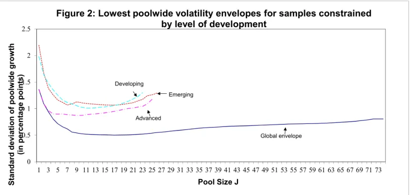
We now generalize the approach. Pools with minimum volatility are not con-strained anymore to include any given country. Figure 2 reports the envelope

of minimal output volatility for all pool sizesJ using the recursive approach

de-scribed in section 2.2. The Figure reports minimal poolwide volatilities across four different samples: pools of up to 74 countries, which traces a “global enve-lope”, and pools within developing, emerging or advanced economies. Across all four samples, the bulk of possible diversification gains is attained with relatively small pools. The global envelope implies the lowest possible poolwide volatility

is 0.50%, and it is obtained in a pool of 17 countries. But volatility is already

as low as 0.62% forJ = 7 along the global envelope. Thus, diversification gains

continue to be achieved within groups consisting of a small number of countries

in this general setup.11

The list of countries involved in minimum-volatility pools confirms that het-erogeneity is key. Interestingly, the list overlaps with that obtained for Chile, which suggests that the sample of countries providing the best hedging prop-erties within a universe of 74 economies is relatively small and robust. The variance-covariance matrix of GDP growth rates contains a few countries with systematically negative off-diagonal elements, i.e. desirable hedging properties.

11

The value reported forJ = 1 corresponds to the standard deviation of the individual GDP growth rate for the least volatile country during the sample period, namely France. Diversification gains for specific countries cannot be easily read off the figure, because the identities of countries involved in pools of different sizes change.

Figure 2 also reports minimum volatilities for three sub-samples: advanced, emerging, and developing countries. Diversification gains remain substantial within each sub-sample, but in all cases the minimum levels of poolwide volatil-ity are substantially higher than in the unconstrained sample. Advanced economies achieve smaller gains, consistent with their lower volatility and internationally correlated business cycles. All four envelopes display the same non-monotonicity

as in Figure 1, with high marginal diversification gains forJ < 10. They turn

negative forJ > 15, when countries with poor hedging properties start being

included.

Figures 1 and 2 help quantify the diversification gains that could accrue to the representative consumer living in a pool of a given size. It captures the decrease in output volatility as pool size increases. This is an input in the welfare gains from pooling risk, which we next evaluate.

3.4

Welfare Gains

This sub-section turns to computing welfareW∗_{. This requires calibrating the}

preference parametersβ, γ and θ, and estimating Mj, Hj, Y0j and ¯M for all

countriesj in any considered pool of size J. The subjective discount rate β is

set at 0.95,θ= 2 andγ= 5. These are later subjected to robustness checks. For

each country and each pool,Mj is computed using consumption data, but ¯M,

Hj, and Y0j are computed using GDP: In autarky, consumption data are used

because they reflect existing sources of insurance, for instance inter-temporal. But in the pool, it is GDP data that must be used, because they reflect the

potential for risk sharing of a given pool of sizeJ.

Growth rates are still constrained to be equal across countries,µj= ¯µ= 3%.

With this constraint, Utj and ¯Utj are never close to zero, and welfare is well

behaved: This will no longer be the case any longer when growth rates are allowed to vary by country. This happens because, as in Lewis (2000), utility may become unbounder under certain parametrizations. Such issues are absent from our sample of 74 countries when GDP growth rates are constant, but do

appear in Section 3.5, where historical growth rates are used to calibrateµj.

Figure 3 reports the highest value ofW∗_{for every pool sizeJ. In the Figure,}

W∗ _{is expressed in percentage of the first best welfare gains obtained with full}

risk sharing worldwide. The results are reported once again for four different

samples. Welfare gains increase monotonically withJ, as they should, with a

maximum for J =N. Just as for volatility, the marginal increases in W∗ _are

largest forJ <10. Marginal gains begin to peter out as soon asJ >7 or 8. This

holds true for the whole sample, but also across the four sub-groups of countries considered, among advanced, emerging, or developing countries. Interestingly, the gains are largest for emerging markets, and smallest for developing countries. This reflects the relative heterogeneity in business cycles in the former group.

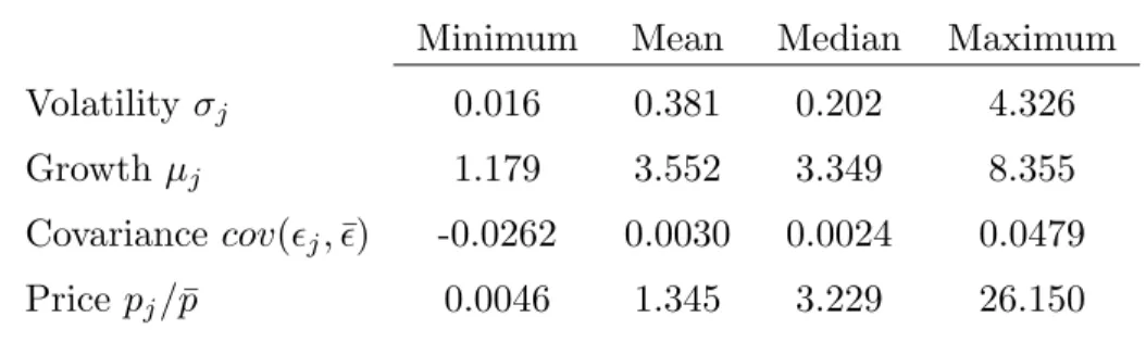
Table 1 reports summary statistics for the key variables serving as inputs to the welfare computations. The Table reports the extrema, mean and median values forσj, µj, cov

εjt,ε¯t

, andpjt / p¯t, for the universe of countries in our

dataset,J = 74. The volatility in GDP growth ranges from 0.01% to 4.32%, with

median 0.20 and mean 0.38. The distribution of country volatilities is slightly

skewed, with a few countries displaying exceptionally volatile business cycles. These are the countries for which risk insurance is particularly desirable. GDP

growth is distributed symmetrically, ranging from 1.18 to 8.35%, with mean and

median values close to each other, around 3.5%. The distribution of the

covari-ances between idiosyncratic and poolwide growth rates is heavily skewed, with

minimum−0.026 and maximum 0.048. There are very few countries with

neg-ative covariances, i.e., very few countries that represent especially good hedges

worldwide. Finally, the relative pricespjt/p¯tare heavily skewed, with a median

percentage share of 3.22, but a mean equal to 1.34%. This reflects that most

countries have very small claims to the worldwide mutual fund, while very few

have large claim, up to 26.15% for J = 74. The distribution of welfare gains is

therefore highly unequal.

Table 2 explores the composition of W∗ _{for various pools. To do so, a}

measure of individual countries’ welfare gains upon entry in the pool, δj, is

introduced. δj satisfies: U0j h C0j(1 +δj), µj, σ2j i =U0j _¯ C0,µ,¯ ¯σ2 . (4)

Similar to Lewis (2000) and Obstfeld (1994),δj is the percent increase in

con-sumption that would make countryj indifferent between autarky and full

risk-sharing in a pool. Table 2 calculatesδjfor all countries for four specific samples,

under the same parametrization as the one used to estimateW∗_.

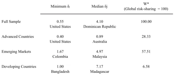
Table 2 reports the minimum value of δj, its median, and the value ofW∗

for four specific pools. The first pool is formed by the entire 74-country sample:

there, δj equals 1.9% of permanent poolwide consumption on average

(unre-ported). But the distribution of δj across the membership is skewed, with a

minimum for the US at 0.50%, and a median for Hong Kong at 6.21%. The

wel-fare consequences of pools are heterogeneous across their membership, reflecting the very heterogeneity of the constituent countries.

Individual country’s welfare gains decrease with per capita income, because they increase with autarkic output volatility. Among advanced economies,

me-dian δj equals 0.89%, whereas it is 4.97% in emerging markets and 7.17% in

developing countries. The distribution of δj is also less dispersed in

homoge-neous pools: for advanced countries, its minimum value is 0.40%, and its

me-dian 0.89%. Contrast this with the dispersion ofδjamong developing countries,

with a minimum of 1.00%, and a median of 7.17%. The heterogeneity in

are positive for all countries, since the minimum gains reported in Table 2 are strictly positive.

How important is carefully chosen diversification in reaping the benefits de-scribed in Figure 3? How do the optimal pools dede-scribed in the Figure differ from alternative groupings of countries, drawn randomly? In Figure 4 we report the welfare gains implied by pools drawn at random. We consider random draws

of 10,000 pools for each value of J. The Figure reports the maximum value of

W∗_{, normalized by the first best welfare gains, as implied by the 10,000 draws,}

along with its 99th _{and 95}th _{percentiles. For ease of comparability, it also}

re-produces the recursive maximum reported in Figure 3. The random maximum

displays a trend increase inJ, with some convexity. As J increases, the gains

fluctuate quite considerably around the trend, reflecting the importance of a few countries in delivering the smooth welfare gains from Figure 3. But the

99th_{and 95}th _{percentiles lose any similitude with the recursive measure: they}

are almost linear inJ, and miss most of the convexity apparent from previous

Figures. In other words, while high values ofW∗ _{can be reached for low values}

ofJ, this only happens in extremely rare groupings of countries. Diversification

gains do not accrue quickly between countries selected at random.

The welfare gains from risk insurance obviously depend on the calibration of preferences, and more specifically on the intertemporal elasticity of substitution. Figures 3 and 4 correspond to specific values of the rate of time preference

β= 0.95, the coefficient of risk aversionγ= 5, andθ= 2, which corresponds to

a relatively low elasticity of intertemporal substitution of 0.5. Unsurprisingly,

the welfare gains of international risk sharing depend on all parameter values: they increase in risk aversion, fall in the intertemporal elasticity, and fall in the rate of time preference. But varying these parameters has symmetric effects on the first best, worldwide welfare gains, and on the poolwide welfare gains.

Since our measures ofW∗ _{are always normalized, the proportional increases we}

document in Figures 3 and 4 are in fact invariant to alternative calibrations of

these three important parameters.12

3.5

Pooling Growth Rates

The previous section computesW∗ _{holding growth rates constant. In principle,}

countries with relatively high expected growth rates should be able to obtain

a higher share of poolwide consumption, with higher values forpj0. In practice

however, the challenges involved in predicting growth rates make it difficult to incorporate differences in expected growth into risk-sharing contracts. For instance, country rankings with respect to growth rates change dramatically from one decade to the next, as shown by Easterly and others (1993). To estimate expected economic growth, this section simply considers the average

12

of historical growth rates over the entire period under consideration. We also assume that individual countries’ growth rates are unaffected by risk sharing.

We estimate µj as the 1975-2004 average of GDP growth in countryj, and ¯µ

as the 1975-2004 average of poolwide GDP growth, for any pool of size J. A

possible concern might be that lower volatility in a pool may create lower mean growth. But this seems unlikely in light of the evidence that lower-volatility countries tend to have relatively high mean growth (Ramey and Ramey, 1995).

So our estimates of W∗ _{on the basis of historical growth rates represent if}

anything a lower bound.

Figure 5 reproduces Figure 3, using historical values forµjand ¯µ. It confirms

the broad pattern of our results: Most marginal gains inW∗ _{accrue forJ <10.}

More than 80% of maximumW∗ _{are reached in pools of 10 countries or fewer.}

In all samples the shape of the envelopes remains the same.

An issue with using historical growth rates is the possibility of zero utility

in the definition ofUtj. We ensure this does not happen by constrainingβMj1−θ

away from 1. In particular, we drop combinations of parameters that result in 0.98 < βM1−θ

j < 1.2. With these constraints, there are no instances of

unbounded utility, or of non-positive prices for any value of covεjt,ε¯t

.This reduces the sample to a maximum of 59 countries, listed in the Appendix, where 3 advanced countries, 7 emerging markets, and 5 developing economies were dropped. There is no reason to expect the dropped countries would be precisely the ones that invalidate the convexity of the welfare function apparent in Figure 5.

It is not apparent from Figure 5, which is normalized, but when growth

rates are country-specific, the levels of W∗ _{shift up for all J - and so do the}

gains from worldwide risk sharing. Such a systematic rise is reminiscent of Obstfeld (1994), who argued international financial integration gives access to high returns, which can have large welfare consequences. In unreported work, we

obtained poolwide weighted averages ofµj, computed for all J. We compared

them with ¯µ, once again computed for all pools. We found little difference

amongst developing countries, some improvement for advanced economies, and largest increases for emerging markets. Historical growth rates are such that it is among emerging markets that growth increases would be most pronounced

for countries participating in a pool. As a result, the increase inW∗ _{is largest}

in this sample.

4

Pooling Risk Within Sub-Samples

The previous section establishes substantial welfare gains are accessible to small pools of countries. Yet risk sharing agreements, or GDP contingent securities, are rarely observed. The reasons for this are not clear (see Borensztein and

Mauro, 2004, for a review). Some authors have suggested that this absence may be due, for example, to difficulties in acquiring information about other countries or in enforcing international contracts, perhaps because of weak institutions.

Such difficulties are summarized byT in Section 2.1; it stands to reason that

the costs implied by such issues should depend on the size and the composition of a pool of risk-sharing countries.

To further explore these issues, we create samples determined by institutional quality or regional proximity, which is often synonymous with strong trade linkages. Goods trade creates incentives to honor international commitments

towards trade partners - often a neighbor in a given region. We computeW∗

for pools of countries that are constrained to belong to the same category, e.g. with high institutional quality.

Then existing regional agreements are considered. These include free-trade agreements, such as the European Union, the ASEAN or Mercosur. We also include pools that were built to provide some degree of cross-country insurance (but clearly fall short of complete risk sharing). We consider the Chiang-Mai Initiative and the Latin American Reserve Fund (FLAR). We illustrate the reduction in consumption volatility that would occur under complete sharing

of GDP risk in the various samples considered. Potential welfare gainsW∗ _are

computed in each case, then compared with the type of welfare gains that could be attained in a pool of identical size, but whose membership would be entirely unconstrained.

4.1

Institutional Quality

We explore the effects of restricting the sample on the basis of default his-tory and scores on the measures of institutional quality that capture contract enforcement. Two definitions are considered. The first, labeled “excellent en-forceability” includes all countries that were in the top half of the distribution of the institutional quality index compiled by Kaufmann et al (2005), and that never experienced severe international repayment difficulties between 1970 and 2004. The second, “above-average institutional quality” is based on the institu-tional quality index only. In addition to advanced countries, the former sample includes four emerging markets and developing countries, whereas the latter includes eight emerging markets and three developing countries.

For each sub-sample, Table 3 reports the median value of aurtakic

consump-tion volatilityσj across the countries j in the sample. Column (2) reports the

minimum variance ¯σthat can be obtained in a pool formed by countries in the

indicated sample, for any pool size. Column (3) reports the medianδj for each

indicated sample, and column (4) reports the corresponding value forW∗_{. The}

Column (1) confirms output volatility is higher in countries with poor

institu-tions. It is 5.24% with low enforceability vs. 2.25% with excellent enforceability,

and 5.45% with institutional quality below average vs. 3.04% if it is above

aver-age. Column (2) suggests the diversification gains from volatility reduction are larger in groups with poor institutions: a decrease of around 4 percentage points

for such groups, as against 1.5 percent for pools with good institutions. This

translates in drastically larger welfare gains for countries with poor institutions

in column (3). The last column in Table 3 reports estimates ofW∗_{. Countries}

with institutions that ensure excellent contract enforceability can only achieve 32% of first-best worldwide risk-sharing gains. But the complementary set of countries, below excellent enforceability, can achieve more than 60% of first-best welfare gains.

The lower panel of Table 3 reports the same statistics, for pools selected on the basis of their regional proximity. We consider three economic zones: the European Union, Asian emerging countries, and Latin American emerging economies. Geographical constraints turn out to be very important for advanced

European countries. With a median volatilityσj of 1.91%, individual country’s

welfare gainsδjare well below 1%. As a result, these pools can hope to achieve at

best 10.15% of first-best welfare gains. The result presumably reflects high cycle

synchronization between rich economies in general, with little diversification to be gained.

The same is not true of emerging markets, with median volatilities σj of

3.93% in Asia and 5.14% in Latin America. Column (2) illustrates that pooled

volatility ¯σcan be reduced to just below 2%. For both groups, individual

coun-try’s median welfare gains are between 3% and 5% of permanent consumption,

and W∗_{doubles to around 20% of first-best welfare. In other words, pooling}

risk among homogeneous European countries carries little gain. Potential gains are substantially larger in (relatively heterogeneous) emerging Asia or emerg-ing Latin America. But either still fall considerably short of what is possible within emerging markets as a whole, or within countries with poor institutions in general.

4.2

Existing Groupings

Finally, we consider the potential welfare gains that would arise if complete risk-sharing were achieved within groups of countries that already exist for other purposes. We include free-trade agreements, whose participants have long-established cooperation, as well as arrangements that involve an element of macroeconomic risk-sharing, such as the Chiang-Mai Initiative and the FLAR. At present, none of these groups explicitly seek to share GDP risk. But we consider them interesting, because their previous history of cooperation and trade and financial relations would presumably make it easier for these groups

to attain the information and mutual trust that would be required to move to

complete risk sharing.13

Table 4 reports the results for several such agreements. Row (1) reports

the median value of country-level autarkic volatility σj for each group. Row

(2) is the value of each pool’s diversified volatility, ¯σP ool, which is then

com-pared with row (3), the minimum value of ¯σ, ¯σM in, that can be achieved

in any, unconstrained pool of similar size J. Row (4) reports the value of

W∗_{corresponding to the volatility reduction implied by the existing pool, ¯σP ool,}

assumingµj= ¯µ= 3%.

Median volatility is highest in groupings that involve emerging markets, in Asia (APEC, ASEAN, Chiang Mai), or in Latin America (FLAR), at around

4.5%. It is much smaller in Europe, at 1.19% in the EMU, or 1.91% in the

EU. Poolwide volatilities decrease substantially for the APEC, Chiang Mai,

and the FLAR, with values between 1.29 and 2.50%. In contrast, volatility

reduction is minimal in Europe. For instance, in the EMU poolwide volatility is equal to its median value across the Union, so that risk sharing would lower consumption volatility for half the membership only. This happens because of the homogeneity in these countries business cycles, and their relatively low volatility.

The values ofW∗ _{mirror these volatility reductions, along with the relative}

sizes of each agreement. ASEAN and FLAR only involve five and seven

coun-tries, respectively. With relatively small reduction in volatility, the values ofW∗

are around five percent of the potential first-best welfare gains. EMU, EU, and

APEC deliver much larger values ofW∗_{, around 30 percent of first-best gains.}

This reflects large values ofJ, equal to 12, 18, and 16, respectively. These

val-ues are consistent with the convexity in Figure 3. The Chiang-Mai grouping is

interesting for a different reason: there are nine participating countries, butW∗

is almost equal to 15 percent of first-best gains. This must be because of the large volatility reduction afforded by this country grouping.

To isolate the relative importance of pool size vs. volatility reduction, the

third row in Table 4 reports the potential volatility reductions that would be

possible in carefully chosen pools of identical sizes, drawn from the full sample of 74 countries. Interestingly, these alternative groupings always deliver substan-tially larger diversification gains in row (3) than in row (2), including for the EMU. Of course, these pools are constituted of countries with much more het-erogeneous business cycles than the groupings in the headings of Table 4. That such small groups of countries can deliver large diversification gains, provided the membership be chosen carefully, is the paper’s main point.

13

For free-trade agreements, on the one hand, trade linkages imply a mutual interest in each other’s economic performance and in honoring of international obligations; on the other hand, trade partners are well known to have synchronized cycles, thus reducing risk-diversification benefits (see, for example, Frankel and Rose, 1998.)

5

Conclusion

Despite a trend toward greater international financial integration, the full gains from complete international risk sharing have hitherto remained elusive. In this paper, we have shown that the bulk of these gains could effectively be reaped in carefully chosen groupings of a small number of economies, often less than ten. This makes it even harder to understand why risk sharing does not arise endogenously. We conjecture it does not because of difficulties in contracting risk sharing agreements between countries. Where such difficulties are likely to be minimal, between countries with good quality institutions, or established trade partners, we show that the potential welfare gains are minimal. In contrast, those small pools that deliver large welfare gains are constituted of economies that are often far away from each other, and include countries with weak institutions or a history of default. Thus, a possible interpretation of our empirical results is that complete risk sharing arrangements have remained elusive because the potential welfare gains may be insufficient to offset obstacles such as concerns about the difficulty of enforcing international contracts.

Advanced Economies [25] Emerging Markets [26] Developing Countries [23] Advanced Europe [18] Emerging Market Latin America [11] Emerging Market Asia [8] Excellent Enforceability [29] Above Average Institutional Quality [37]

Australia Argentina* Algeria* Austria Argentina China Australia Australia Austria Brazil Bangladesh Belgium Brazil India Austria Austria Belgium Chile Benin Denmark Chile Indonesia Belgium Belgium Canada China Bolivia Finland Colombia Korea Botswana Botswana Hong Kong SAR Colombia Botswana France Dom. Rep. Malaysia Canada Brazil Denmark* Cote d'Ivoire* Cameroon Germany Ecuador Pakistan Denmark Canada Finland Dom. Rep. Congo Rep. Greece El Salvador Philippines Finland Chile France Ecuador Costa Rica Iceland Mexico Thailand France Costa Rica Germany Egypt Gabon Ireland Peru Germany Denmark Greece El Salvador* Gambia Italy Uruguay Greece Finland Iceland Hungary Ghana Luxembourg Venezuela Hong Kong France Ireland India Guatemala Netherlands Hungary Germany Italy Indonesia Kenya Norway Iceland Greece Japan Korea Lesotho Portugal Ireland Hong Kong SAR Luxembourg Malaysia Madagascar* Spain Italy Hungary Netherlands Mexico Malawi Sweden Japan Iceland New Zealand* Morocco Nicaragua Switzerland Luxembourg Ireland Norway Pakistan Paraguay United Kingdom Malaysia Italy Portugal Peru* Rwanda* Netherlands Japan Singapore Philippines Senegal New Zealand Korea Spain South Africa Syria Norway Luxembourg

Sweden Thailand Togo* Portugal Malaysia

Switzerland* Tunisia Trin. and Tob.* Singapore Morocco United Kingdom Uruguay* SouthAfrica Netherlands United States Venezuela* Spain New Zealand

Zimbabwe* Sweden Norway

Switzerland Portugal United Kingdom Singapore United States South Africa

Spain Sweden Switzerland Thailand Trinidad and Tobago United Kingdom United States Uruguay Appendix Table 1: Country Samples

Notes: Advanced countries are defined as in the International Monetary Fund’s World Economic Outlook. The

remaining countries are emerging if they are included in either the stock-market based International Financial Corporation’s Major Index (2005) or JPMorgan’s EMBI Global Index (2005), which includes countries that issue bonds on international markets. The remaining countries are classified as developing. Above average institutional quality is according to the index of Kaufmann, Kraay, and Mastruzzi (2005). Excellent enforceability is defined as above average institutional quality and no defaults on international debt in 1970-2004 according to Detragiache and Spilimbergo (2001) and Reinhart, Rogoff and Savastano (2003). GDP data in current U.S. dollars are from the IMF’s World Economic Outlook.) GDP data at PPP are from the World Bank’s World Development Indicators. Stars denote countries that are excluded to preserve stationarity in Section 3.5.

APEC [16] ASEAN [5] CHIANG MAI [9] EMU [12] EU [18] FLAR [7] Australia Indonesia China Austria Austria Bolivia Canada Malaysia Hong Kong Belgium Belgium Colombia Chile Philippines Indonesia France Denmark CostaRica China Singapore Japan Germany Finland Ecuador Hong Kong Thailand Korea Greece France Peru Indonesia Malaysia Ireland Germany Uruguay Japan Philippines Italy Greece Venezuela Korea Singapore Luxembourg Iceland

Malaysia Thailand Netherlands Ireland

Mexico Portugal Italy

New Zealand Spain Luxembourg

Peru Switzerland Netherlands

Philippines Norway

Singapore Portugal

Thailand Spain

United States Sweden

Switzerland United Kingdom

Appendix Table 2: Additional Country Samples

References

Backus, David K., and Gregor W. Smith, 1993, “Consumption and real exchange rates in dynamic economies with non-traded goods,” Journal of Inter-national Economics, November, Vol. 35, No. 3-4, pp. 297–316.

Baxter, Marianne, and Michael A. Kouparitsas, 2005, “Determinants of busi-ness cycle comovement: a robust analysis,” Journal of Monetary Economics, January, Vol. 52, No. 1, pp. 113–157.

Borensztein, Eduardo R., and Paolo Mauro, 2004, “The Case for GDP-Indexed Bonds,” Economic Policy, April, Vol. 19, No. 38, pp. 165–216.

Brennan, Michael and H. Henry Cao, 1997,“International Portfolio Invest-ment Flows,” Journal of Finance, December, Vol. 52, No. 5, pp. 1851-1880.

Coeurdacier, Nicolas, 2009, “Do trade costs in goods market lead to home bias in equities?”, 2009, Journal of International Economics, 77, 86-100.

Cole, Harold L., and Obstfeld, Maurice, 1991, “Commodity trade and in-ternational risk sharing: How much do financial markets matter?”, Journal of Monetary Economics, August, Vol. 28, pp.3–24.

Doyle, Brian and Jon Faust, 2005, “Breaks in the Variability and Co-Movement of G-7 Economic Growth”, Review of Economics and Statistics, Vol. 87, No. 4, pp. 721-740.

Easterly, William, Michael Kremer, Lant Pritchett, and Lawrence H. Sum-mers, 1993, “Good policy or good luck? Country growth performance and temporary shocks,” Journal of Monetary Economics, Vol. 32, pp. 459–483.

Eichengreen, Barry, 2007, “Insurance Underwriter or Financial Development Fund: What Role for Reserve Pooling in Latin America?” Open Economies Review, Vol. 18, No. 1, pp. 27-52

Eichengreen, Barry, and Charles Wyplosz, 1993, “The Unstable EMS,” Brookings Papers on Economic Activity, No. 1, pp. 51–143.

Epstein, Larry and Stanley Zin, 1989, “Substitution, Risk Aversion and the Temporal Behavior of Consumption and Asset Returns: A Theoretical Frame-work”, Econometrica, Vol. 57, No. 4, pp. 937–969.

Frankel, Jeffrey A., and Andrew K. Rose, 1998, “The Endogeneity of the Optimum Currency Area Criteria,” Economic Journal, July, Vol. 108, No. 449, pp. 1009–25.

Han, Qiaoming, Yinyu Ye, and Jiawei Zhang, 2002, “An Improved Round-ing Method and Semidefinite ProgrammRound-ing Relaxation for Graph Partition,” Mathematical Programming, Vol. 92, No. 3, pp. 509–535.

Imbs, Jean and Paolo Mauro, 2007, “Pooling Risk Among Countries”, IMF Working Paper 07/132.

Kalemli-Ozcan, Sebnem, Bent Sorensen, and Oved Yosha, 2001, ”Economic integration, industrial specialization, and the asymmetry of macroeconomic fluc-tuations”, Journal of International Economics 55 (1), 107-137

Kang, Jun-Koo, and Rene Stulz, 1997, “Why is there a home bias? An analysis of foreign portfolio equity ownership in Japan,” Journal of Financial Economics, 46(1), pp. 3-28.

Kaufmann, Daniel, Aart Kraay, and Massimo Mastruzzi, 2005, “Gover-nance Matters IV: Gover“Gover-nance Indicators for 1996–2004,” The World Bank, http://www.worldbank.org/wbi/governance/govdata/.

Lewis, Karen K., 2000, “Why Do Stocks and Consumption Imply Such Dif-ferent Gains from International Risk Sharing?” Journal of International Eco-nomics, Vol. 52, pp. 1–35.

Lewis, Karen K., and Edith Liu, forthcoming, “Evaluating International Consumption Risk Sharing Gains: An Asset Return View”, Journal of Monetary Economics.

Lucas, Robert E., Jr., 1987, Models of Business Cycles (Oxford: Blackwell Publishers).

Merton, Robert C., 1990, “The Financial System and Economic Perfor-mance,” Journal of Financial Services Research, Vol. 4, No. 4, pp. 263–300.

Merton, Robert C., 2002, “Future Possibilities in Finance Theory and Fi-nance Practice.” In Mathematical FiFi-nance - Bachelier Congress 2000, edited by H. Geman, D. Madan, S. Pliska, and T. Vorst. Berlin: Springer-Verlag.

Obstfeld, Maurice, 1994, “Evaluating Risky Consumption Paths: The Role of Intertemporal Substitutability,” European Economic Review, Vol. 38, No. 7, pp. 1471–86.

Pallage, Stephane, and Michel Robe, 2003, “On the Welfare Cost of Eco-nomic Fluctuations in Developing Countries,” International EcoEco-nomic Review, Vol. 44, No. 2, pp. 677–698.

Park, Yung Chul, and Yunjong Wang, 2005, “The Chiang Mai Initiative and Beyond,” The World Economy, Vol. 28, No. 1, pp. 91–101.

Ramey, Garey, and Valerie A. Ramey, 1995, ”Cross-Country Evidence on the Link between Volatility and Growth,” American Economic Review, December, Vol. 85, No. 5, pp. 1138–51.

Ravn, Morten O., 2001, “Consumption Dynamics and Real Exchange Rate,” CEPR Discussion Papers 2940.

Shiller, Robert J., 1993, Macro Markets: Creating Institutions for Managing Society’s Largest Economic Risks (Oxford: Oxford University Press, Clarendon Series).

Solnik, Bruno, 1974, “Why Not Diversify Internationally Rather Than Do-mestically?” Financial Analysts Journal, pp. 48–54.

Tesar, Linda, 1995, ”Evaluating the Gains from International Risksharing,” Carnegie-Rochester Conference Series on Public Policy 42, pp. 95-143.

Table 1: Summary Statistics for J=74

Minimum

Mean

Median

Maximum

Volatility

σ

0.016

0.381

0.202

4.326

Growth

µ

1.179

3.552

3.349

8.355

Covariance

cov

(

ǫ

,

¯

ǫ

)

-0.0262

0.0030

0.0024

0.0479

Price

p

/

p

¯

0.0046

1.345

3.229

26.150

Notes: Summary statistics for the universe of 74 countries. cov(ǫj,¯ǫ) denotes the covariance between individual countries and poolwide growth rates. The price ratio pj/p¯is defined in equations (9) and (10). All values are in percentages. Real GDP and consumption data are from the World Bank’s World Development Indicators.

Minimum δj Median δj

W* (Global risk-sharing = 100)

Full Sample 0.55 4.10 100.00

United States Dominican Republic

Advanced Countries 0.40 0.89 28.33

United States Australia

Emerging Markets 1.67 4.97 57.51

Colombia Malaysia

Developing Countries 1.00 7.17 6.58

Bangladesh Madagascar

Table 2: Welfare Gains

Notes: Minimum, median, and total welfare gains for sub-samples indicated, assuming the same expected growth (3 percent) across countries. The results assume θ=2, γ=5, and β=0.95. Country lists are provided in the Appendix. GDP data are from the World Bank’s World Development Indicators.

(1) (2) (3) (4) Median σj individual country Minimum poolwide variance Median δj W*( % worldwide risk-sharing)

All countries (pooling with any country) 4.49 0.54 6.21 100.00

Costs of weak enforcement

Excellent enforceability countries (pooling only with excellent

enforceability countries) 2.25 0.87 1.73 32.21

Below excellent enforceability countries (pooling only with below

excellent enforceability countries) 5.24 1.30 8.77 60.89

Above average inst. countries (pooling with only above average inst.

countries) 3.04 0.82 2.65 44.67

Below average inst. countries (pooling with only below average inst.

countries) 5.45 1.50 9.96 48.64

Costs of regional constraints

European Union (pooling only with EU) 1.91 1.05 0.68 10.15

Asian emerging (pooling only with Asian emerging) 3.93 1.84 2.98 18.18

Latin American emerging (pooling only with Latin American emerging) 5.14 1.90 4.96 21.56

Table 3: Gains from Risk Pooling Among Countries

Notes: Column (1) reports the median of σj (across countries in the indicated sub-sample). Column (2) reports the median of the lowest possible standard deviation of poolwide growth (across countries in the indicated sub-sample). Column (3) reports the median δj (across countries in the indicated sub-sample) assuming growth rates fixed at 3 percent per annum. Column (4) reports W*, assuming growth fixed at three percent per annum.

Table 4. Poolwide Volatility and Welfare for Selected Groups

APEC

ASEAN

CHIANG MAI

EMU

EU

FLAR

Median

σ

4.44

4.53

4.48

1.19

1.91

4.62

¯

σ

1.29

3.47

1.40

1.19

1.09

2.50

¯

σ

0.68

0.86

0.79

0.66

0.65

0.71

W

∗

29.05

5.25

14.50

29.71

32.17

5.67

(worldwide = 100)

Notes: Median country volatilityσj , poolwide volatility ¯σP ool , and minimum poolwide volatility

¯

σM in that can be achieved in any, unconstrained pool with the same number of countries J. The

welfare gains W∗ use ¯σP ool. Growth is set at 3 percent, θ = 2, γ = 5, and β = 0.95. The

list of countries in each sample is in the Appendix. GDP data are from the World Bank’s World Development Indicators.

Chile drawing partners from whole sample Chile pooling with Emerging

Markets (EM)

Chile pooling with Lat. Am. EMs

Chile pooling with advanced economies Chile's worst pool

0 1 2 3 4 5 6

1

3

5

7

9 11 13 15 17 19 21 23 25 27 29 31 33 35 37 39 41 43 45 47 49 51 53 55 57 59 61 63 65 67 69 71 73

Pool Size J

Figure 1. Benefits of diversification under various restrictions:

The case of Chile

Notes: The figure reports the standard deviation of the growth rate of aggregate (poolwide) GDP for the pool (of each size) that yields the lowest standard deviation (or the highest, in the case of the top line). Each group is constrained to contain Chile. GDP data at purchasing power parity are drawn from the World Bank’s World Development Indicators. The pool yielding the lowest (or highest) standard deviation is found by checking all possible combinations of countries for each J and

Global envelope Advanced Emerging Developing 0 0.5 1 1.5 2 2.5 1 3 5 7 9 11 13 15 17 19 21 23 25 27 29 31 33 35 37 39 41 43 45 47 49 51 53 55 57 59 61 63 65 67 69 71 73 St a n d a rd d e v ia ti o n o f p o o lw id e g ro w th (in percent a ge point s) Pool Size J

Figure 2: Lowest poolwide volatility envelopes for samples constrained

by level of development

Notes: The figure reports the standard deviation of the growth rate of poolwide GDP for the pool (of each size) that yields the lowest standard deviation for each sub-sample. The pool yielding the lowest standard deviation is found by checking all possible combinations of countries and by running the approximation procedure described in the text. GDP data are from the World Bank’s World Development Indicators.

Developing

Countries

Emerging

Markets

Advanced

Countries

Full

Sample

To

ta

l

w

e

lf

a

re

g

a

in

s

(w

orl

d

w

id

e

ris

k-sha

ring

=

10

0)

Pool Size J

Figure

3:

Pooling

Gains

Notes: For each pool size, the figure reports the highest possible value for W∗ using the procedure described in the text. Welfare gains are computed assumingγ= 5, β= 0.95,θ= 2, and a constant growth rate of three percent for all countries and

Max.

from

recursive

search

procedure

Max.

from

10,000

draws

99th

pctile

from

10,000

draws

95th

pctile

from

10,000

draws

To

ta

l

we

lf

ar

e

ga

in

s

(w

or

ldwide

ri

sk

Ͳ

sha

ring

=

10

0)

Figure

4:

Random

Pools

and

Actual

Gains

Notes: For each pool size, the figure reports the highest possible value for W∗ using the procedure described in the text. In addition, the figure reports the maximum, 99th percentile, and 95th percentile obtained from 10,000 random pool draws. Welfare gains are computed using the W∗ formula given in the text assuming γ = 5, β = 0.95, θ = 2 and a constant growth rate of three percent for all countries and pools. GDP data are from the World Bank’s World

Developing

Countries

Emerging

Markets

Advanced

Countries

Full

Sample

To

ta

l

w

e

lf

a

re

g

a

in

s

(w

o

rld

w

ide

ri

sk-sh

aring

=

10

0)

Pool Size J

Figure

5:

Pooling

Gains

(Country

Ͳ

Specific

Growth

Rates)

Notes: The figure reports the highest possible values forW∗ using the search procedure and the formula described in the text. The results assumeγ= 5,β= 0.95,θ= 2, and country-specific growth rates, given by their historical means. GDP data are from