Multilevel thresholding hyperspectral image segmentation
based on independent component analysis and swarm
optimization methods
Murinto a,1,*, Nur Rochmah Dyah Puji Astuti a,2, Murein Miksa Mardhia a,3
a Informatics Department, Universitas Ahmad Dahlan, Yogyakarta, Indonesia
1[email protected]; 2 [email protected]; 3 [email protected]
* corresponding author
1.
Introduction
A hyperspectral image is an image that has hundreds of bands with very high spectral resolution. It’s range from visible light to infrared [1]. Hyperspectral image is very suitable for images classification from the earth's surface because of very detailed. In the recent years, many researchers use hyperspectral image for their research, and the results are satisfying. The problem faced when using hyperspectral image data is its high dimensions, so the calculation process takes a long time. The transformation image dataset from original dataset is often used to describe dataset in order to obtain a relatively simple method of calculation. Some well-known linear transformation methods are principal component analysis (PCA) [2][3], linear discriminant analysis (LDA) [4]. The PCA method, independent component analysis (ICA) [5]–[7], discriminant independent component analysis (DICA) [8] and non-negative matrix factorization (NMF) [9] have been widely used for low-dimensional feature extraction from sensory raw data.
Reducing the dimensions of high data to a lower dimension of data is the existence of a problem of 'curse of dimensionality'. This event resulted in changes in dimensions which tended to increase exponentially. High-dimensional data when processed directly will result in long processing times and tend to require expensive costs. Some data dimension reduction techniques that are used by researchers A R T I C L E I N F O A B S T R A C T
Article history
Received December 30, 2018 Revised March 14, 2019 Accepted March 26, 2019 Available online March 31, 2019
High dimensional problems are often encountered in studies related to hyperspectral data. One of the challenges that arise is how to find representations that are accurate so that important structures can be cleared easily. This study aims to process segmentation of hyperspectral image by using swarm optimization techniques. This experiments use Aviris Indian Pines hyperspectral image dataset that consist of 103 bands. The method used for segmentation image is particle swarm optimization (PSO), Darwinian particle swarm optimization (DPSO) and fractional order Darwinian particle swarm optimization (FODPSO). Before process segmentation image, the dimension of the hyperspectral image data set are first reduced by using independent component analysis (ICA) technique to get first independent component. The experiments show that FODPSO method is better than PSO and DPSO, in terms of the average CPU processing time and best fitness value. The PSNR and SSIM values when using FODPSO are better than the other two swarm optimization methods. It can be concluded that FODPSO has better in order to obtain segmentation results compared to the previous method.
This is an open access article under the CC–BY-SA license.
Keywords
Darwinian particle swarm Optimization
FODPSO
Hyperspectral Image Multi-level thresholding Particle swarm optimization
include principal component analysis (PCA), linear discriminant analysis (LDA), and independent component analysis (ICA) [10]–[13].
ICA extracts a series of statistically independent features, where this application is broad in the field of blind signal separation and feature extraction. Some approaches that have been used to extract ICA features include Infomax and the most popular FastICA algorithm. The Infomax algorithm works by maximizing entropy which is transformed non-linearly from the ICA network output, FastICA originates an update rule by maximizing the negentropy of ICA network output.
A process of dividing digital images into several regions or objects is namely image segmentation. The object provides more information that is more useful than just single pixels. Image segmentation plays an important role in remote sensing analysis. For example, when we want the classification result to increase, classification that integrated spectral and spatial information, segmentation process needs to be done [14]–[16]. One method of image segmentation that is often used is thresholding [17]. There are two types of thresholding technique, namely property-based thresholding and optimal thresholding methods. Several techniques have been proposed that are related to optimal thresholding using bi-level thresholding which can eventually be expanded into multi-level thresholding. One of techniques that is widely used is bio-inspired algorithms, namely particle swarm optimization (PSO) [18][19], Darwinian PSO derivatives (DPSO) [20], and Fractional Orders DPSO (FODPSO) which is a special case of the DPSO by Pires et al. [21] and Couceiro et al. [22].
This study aims to conduct a better process of the segmentation of hyperspectral image data through the application of the ICA dimension reduction method and the use of swarm optimization (PSO, DPSO, and FODPSO) techniques to segment hyperspectral image dataset. In addition, this study will evaluate the three swarm optimization techniques, which technique is better when used in the process of segmentation of hyperspectral images through segmentation evaluation.
2.
Method
2.1.Multi-level Thresholding Image Segmentation
The first step to success in the object recognition is segmentation. The quality of the end product depends largely on quality of segmentation method itself. There are various kinds of techniques for image segmentation. Commonly, segmentation techniques can be classified in thresholding, edge-based, region growing and clustering methods [23][24]. Thresholding in an image for a certain T threshold will partition image I into different subregions based on the value of T. In a non-parametric approach, the threshold is determined to ensure that the image histogram meets criteria based on inter-class variance [25] or based on entropy criteria [26].
At bi-level thresholding, the pixels of gray level image below the value of Th will be assigned to one group K0, while m pixels t with gray levels above Th, will be included in another group, K1. At the end
of the thresholding process I image will be grouped into two groups. If I image is assumed to be represented by the L gray level, then the bi-level thresholding can be defined as the equation:
K0= {g(x, y) ∈ I|0 ≤ g(x, y) ≤ Th − 1} (1)
K1= {g(x, y) ∈ I|0 ≤ g(x, y) ≤ Th − 1} (2)
Multilevel thresholding uses more than one threshold value and produces an image with several groups.
K0= {g(x, y) ∈ I|0 ≤ g(x, y) ≤ Th1− 1} K1= {g(x, y) ∈ I|Th1≤ g(x, y) ≤ Th2− 1} Ki = {g(x, y) ∈ I|Thi≤ f(x, y) ≤ Thi+1− 1}
Kn= {g(x, y) ∈ I|Thn≤ f(x, y) ≤ L − 1} where 𝑇ℎ𝑖 = 1,2, . . , 𝑛 the threshold value, while is n is the number of thresholds.
The Otsu method is a non-parametric method used in image segmentation. Imagery is divided into different classes so that the variance between the classes is maximal. In his research, Otsu [25] defines variance between classes as the sum of Sigma functions of each class, which are written as equations:
𝑔(𝑡) = 𝜎0+ 𝜎1 (7)
𝜎0= 𝑤0+ (𝜇0− 𝜇𝐴)2, 𝜎1= 𝑤1+ (𝜇1− 𝜇𝐴)2(8)
where 𝜇𝑇 is average of intensity original image. Mean level n bi-level thresholding for each class (𝜇𝑖)is
written as: 𝜇0= ∑ 𝑖𝑝𝑖 𝑤0 𝑇−1 𝑖=0 𝜇1= ∑ 𝑖𝑝𝑖 𝑤1 𝐿−1 𝑖=𝑇
The optimal threshold is obtained from the maximization function between class variances, which is written as an equation:
𝑇∗= 𝑎𝑟𝑔𝑚𝑎𝑥𝑔(𝑡) (11)
In the multi-level thresholding problem, the Otsu method can be written as:
𝜎0= 𝑤0+ (𝜇0− 𝜇𝐴)2 (12)
𝜎1= 𝑤1+ (𝜇1− 𝜇𝐴)2 (13)
𝜎𝑗= 𝑤𝑗+ (𝜇𝑗− 𝜇𝐴)2 (14)
𝜎𝑚= 𝑤𝑚+ (𝜇𝑚− 𝜇𝐴)2 (15)
In multi-level thresholding, mean level value of each class (𝜇𝑖) can be written as:
𝜇0= ∑ 𝑖𝑝𝑖 𝑤0 T1−1 𝑖=0 (16) 𝜇1= ∑ 𝑖𝑝𝑖 𝑤1 T2−1 𝑖=T1 (17) 𝜇𝑗= ∑ 𝑖𝑝𝑖 𝜇𝑗 Tj+1−1 𝑖=𝑇𝑗 (18) 𝜇𝑚= ∑ 𝑖𝑝𝑖 𝜇𝑛 L−1 𝑖=Tn (19)
The optimal threshold value is obtained by maximizing variance among existing classes, which are written as equations:
𝑇∗= 𝑎𝑟𝑔𝑚𝑎𝑥(∑ 𝜎 𝑖 𝑛
2.2.Swarm Optimization Methods
2.2.1. Particle Swarm Optimization (PSO)
Particle swarm optimization (PSO) technique was first introduced by Kennedy and Eberhart [18]. PSO is included in a type of stochastic based optimization that mimics the behavior of a group of flocks or birds or social behavior in a group of living things. The basic idea of PSO is to involve a scenario where a flock of birds in search of food sources in an area. All birds do not know exactly where the food is located. In the each iteration they will find out how far the food will be found. The best strategy will be followed by birds that are close to food and also from the best position previously achieved. PSO is built with the concept of optimization through a particle swarm. PSO is included in one of the multi-agent based parallel search techniques. A swarm particle is maintained and each particle represents a parallel solution in a swarm. The whole particle will fly in a multidimensional search space through adjusting their position and speed based on the experiences of themselves and their neighbors.
The original PSO algorithms are written in the form of speed update equations (position updated) and position updates [19] as shown in equations (21) and equation (22) respectively.
𝑣𝑖𝑗𝑡+1= 𝑣𝑖𝑗𝑡 + 𝑐1𝑟1𝑗𝑡 ∗ (𝑃𝑏𝑒𝑠𝑡,𝑖𝑡 − 𝑥𝑖𝑗𝑡) + 𝑐1𝑟2𝑗𝑡 ∗ (𝐺𝑏𝑒𝑠𝑡− 𝑥𝑖𝑗𝑡)
𝑥𝑖𝑗𝑡+1= 𝑥𝑖𝑗𝑡 + 𝑣𝑖𝑗𝑡+1
The algorithm is controlled through individual experience (best position), and overall experience (best global) and current movements of particles to determine their next position in the search space. Experiences are accelerated through two factors of acceleration constants 𝑐1 and 𝑐2 and two random
numbers𝑟1, 𝑟2 that are generated with range values between 0 and 1. Population initials (swarm) are N
size and dimension D is denoted as 𝑥 = [𝑥1, 𝑥2, . . , 𝑥𝑁]𝑇. Each individual (particle) 𝑥𝑖(𝑖 =
1,2,3, … , 𝑁)given as𝑥𝑖 = [𝑥𝑖1, 𝑥𝑖2, … , 𝑥𝑖𝐷], the initial velocity is denoted as 𝑣 = [𝑣1, 𝑣2, . . , 𝑣𝑁]𝑇.Then,
the velocity of each particle 𝑥𝑖(𝑖 = 1,2,3, … , 𝑁)given as𝑣𝑖 = [𝑣𝑖1, 𝑣𝑖2, … , 𝑣𝑖𝐷]. While i index have
values from 1 to N and j index have values from 1 to D.
In equation (21) consists of three parts, namely the first part, is part of momentum. The speed changes from the current speed without being sudden. This section increases the global search capabilities of particles through prevention so that particles do not converge too fast. The second part is a cognitive part that represents how particles learn from flying experiences that have been done before. The third part is a social part that represents how the particles learn from the learning experience of the group.
The basic modification of the PSO algorithm that is usually carried out includes how to increase the speed of convergence, control trade-offs of exploration and exploitation, overcome the problems of stagnation of convergence or premature, flanking techniques, technique of boundary value problems, initial and final conditions. In PSO, particle speed is very important. At each step of the PSO process, all particles are processed through speed adjustments for each particle movement in each dimension of the search space. There are two characteristics in PSO, namely exploration and exploitation. Exploration is the ability to explore different areas in the search space in order to get optimal good, while exploitation is the ability to focus searches in the search area to improve expected solutions. When the speed increases, the position of the particles will be updated quickly.
2.2.2. Darwinian Particle Swarm Optimization (DPSO)
A common problem with the optimization algorithm is to get stuck on the optimal local. Certain algorithms can work well on one problem but may fail on another. In the implementation of the PSO, a flock of completion of the test is utilized. For applying natural selection with a single herd, the algorithm must detect when stagnation has occurred. In searching for a natural selection model that is better to use the PSO algorithm, a derivative of PSO named Darwinian Particle Swarm Optimization (DPSO) is introduced by Tillet et al. [20]. Many researcher have been using DPSO methods in their
research [14], [15], [27]. Each swarm individually performs like a normal PSO algorithm where natural selection (Darwinian principles of survival of the fittest) is used to increase the ability to distance themselves from local optima. When search tends to be optimal locally, searches in that area are only discarded and other regions are searched instead. In this approach, at each step, the herd that gets better is rewarded (extending the life of the particle or spawning new offspring) and the herd stagnates (reducing the life of the herd or removing particles). To analyze the general state of each herd, the suitability of all particles is evaluated and the environment and the best individual position of each particle are updated. If a new global solution is found, new particles will appear. Particles are removed if the flock fails to find the conditions more suitable for a number of steps specified.
Some simple rules are followed to remove flocks, remove particles, and spawn new flocks and new particles: i) when the herd population is below the minimum, the herd is removed; and ii) the worst performing particles in the herd are removed when the maximum number of steps (counter search
𝑆𝐶𝑐𝑚𝑎𝑥) without increasing the fitness function is reached. After the removal of particles, instead of
being set to zero, the counter is reset to a value close to the threshold number, according to the equation: 𝑆𝐶𝑐(𝑁𝑘𝑖𝑙𝑙) = 𝑆𝐶𝑐𝑚𝑎𝑥[1 −
1
𝑁𝑘𝑖𝑙𝑙+1] (22)
Where is 𝑁𝑘𝑖𝑙𝑙 as the number of particles removed from swarms during periods where there is no
increase in fitness. To spawn a new herd, a swarm of particles must never be removed and the maximum number of herds cannot be exceeded. However, new herds are only made with probabilities p = f / NS, with f are random numbers in [0, 1] and NS number of herds. This factor avoids the creation of new herds when there are many herds. A particle pops up whenever a swarm of swarm reaches a new global best and a maximum population defined from a new swarm is not reached.
2.2.3. Fractional Order Darwinian Particle Swarm Optimization (FODPSO)
Fractional order Darwinian particle swarm optimization (FODPSO) introduced by Pires et al. [21]. This method is one of the extensions of Darwinian particle swarm optimization (DPSO). DPSO technique is based on fractional calculus (FC). The fractional concept is a derivative of Grunwald Letnikov, where is equation can be written as in (23) [21].
𝐷𝛼[𝑦(𝑡)] = lim 𝑖=0[ 1 𝑖𝛼∑ (−1)𝑚Γ(𝛼+1)𝑦(𝑡−𝑚𝑖) Γ(𝑚+1)Γ(𝛼−𝑚+1) ∞ 𝑚=0 ] (23)
where 𝛼 is fractional coefficient, 𝛼 ∈ 𝐶 fractional coefficient, Γ is the Gamma function and y (t) is a signal. In discrete time, a signal 𝐷𝛼[𝑦(𝑡)]is defined as Equation (24).
𝐷𝛼[𝑦(𝑡)] = 1 𝑇𝛼∑ (−1)𝑚Γ(𝛼+1)𝑦(𝑡−𝑚𝑇) Γ(𝑚+1)Γ(𝛼−𝑚+1) 𝑟 𝑚=0 (24)
A sample period is represented by T and r which is the 'truncate'. From PSO equation (21) is obtained from FODPSO as written equation (25).
𝐷𝛼[𝑣𝑖+1𝑛 ] = 𝑐1𝑟1(𝑔̅𝑖𝑛− 𝑥𝑖𝑛) + 𝑐2𝑟2(𝑥̅𝑖𝑛− 𝑥𝑖𝑛) + 𝑐3𝑟3(𝑛̅𝑖𝑛− 𝑥𝑖𝑛) The FODPSO speed update equation becomes the equation (26).
𝑣𝑖+1𝑛 = 𝛼𝑣𝑖𝑛+ 1 2𝛼𝑣𝑖−1 𝑛 +1 6𝛼(1 − 𝛼)𝑣𝑖−2 𝑛 + 1 24𝛼(1 − 𝛼)(2 − 𝛼)𝑣𝑖−3 𝑛 + 𝑐 1𝑟1(𝑔̅𝑖𝑛− 𝑥𝑖𝑛) + 𝑐2𝑟2(𝑥̅𝑖𝑛− 𝑥𝑖𝑛) + 𝑐3𝑟3(𝑛̅𝑖𝑛− 𝑥𝑖𝑛) The DPSO is seen as a special case from FODPSO where𝛼 = 1.
2.3.Evaluation of Performance
Evaluation of performance for optimization algorithm used in image segmentation in the proposed research will be compared through several quality measure values [28]–[31]. First, measuring of the similarity segmented images and reference images (pre-segmented imagery) is used the peak signal to noise ratio (PSNR) index, which is based on the results of the MSE (mean square error), where MSE is calculated from the average squared intensity original image and pixel image produced. The values of MSE and PSNR are defined in equations (27) and equations (28).
𝑀𝑆𝐸 = 1 𝑀𝑁∑ ∑ (𝑥(𝑖, 𝑗) − 𝑦(𝑖, 𝑗)) 2 𝑁 𝑗=1 𝑀 𝑖=1 (27)
where the original image represented by 𝑥(𝑖, 𝑗) and the segmented image represented by 𝑦(𝑖, 𝑗). Whereas the pixel position image represented by i and j that has the size of M x N. A mathematical measure of image quality is Signal-to-noise ratio (SNR) that is based on the difference in pixels between two images. The size of the SNR is an estimate of the image quality of the segmentation compared to the original image. PSNR is defined as equation (28).
𝑃𝑆𝑁𝑅(𝑑𝐵) = 10𝑙𝑜𝑔10
𝑠𝑛
𝑀𝑆𝐸 (28)
where s=255 for an 8-bit image (grayscale). PSNR is basically an SNR when all pixel values are the maximum possible value [32]. Second, the Structural similarity index metric (SSIM) index introduced by Wang (2002) introduces where the average of the structural similarity index is calculated as follows: (i). The original image and segmentation image are divided into 8 x 8 size blocks and then the block is
converted into vector-vector.
(ii). Two Means and two Standard deviations and one covariance are calculated using equations (29), (30) and (31). 𝜇𝑥= 1 𝑁∑ 𝑥𝑖 𝑁 𝑖=1 , 𝜇𝑦= 1 𝑁∑ 𝑦𝑖 𝑁 𝑖=1 (29) 𝜎𝑥2= 1 𝑁−1∑ (𝑥𝑖− 𝑥̅) 2 𝑁 𝑖=1 , 𝜎𝑦2= 1 𝑁−1∑ (𝑦𝑖− 𝑦̅) 2 𝑁 𝑖=1 (30) 𝜎𝑥𝑦= 1 𝑁−1∑ (𝑥𝑖− 𝑥̅)(𝑦𝑖− 𝑦̅) 𝑁 𝑖=1 (31)
(iii).Structural similarity index metric (SSIM) between image x and image y are computed using equation (32).
𝑆𝑆𝐼𝑀(𝑥, 𝑦) = (2𝜇𝑥𝜇𝑦+𝑐1)(2 𝜎𝑥𝑦+𝑐2)
(𝜇𝑥2+𝜇𝑦2+𝑐1)(𝜎𝑥2+𝜎𝑦2+𝑐1) (32)
where 𝑐1and𝑐2are constants.
3.
Results and Discussion
Experiments of fitness criteria based on between-class variance are maximized to build optimal image segmentation. PSO, DPSO, and FODPSO use the same criteria. Multi-level thresholding of image segmentation is done using these three techniques. In Table 1 the fitness ratio and optimal threshold values of Aviris Indian Pines imagery are obtained from PSO, DPSO, and FODPSO techniques in the between-class variance (Otsu’s problem) criteria. While Table 2 shows the PSNR and SSIM values for Aviris Indian Pines Image that have been done in this experiment. In this experiment m is a level threshold.
Table 1 shown that when the level used is m = 2 for Indian Pines Aviris image dataset, the fitness value for the PSO, DPSO and FODPSO method is 1.1857, the optimal threshold is 133. While at level m = 12, the fitness value for the three methods the value is 1.2988 while the optimal threshold value varies for the three methods
Table 1. Comparison of Fitness and Threshold Values Using PSO, DPSO and FODPPSO Methods for Otsu’s criteria for Aviris Indian Pines Image
Level (m)
Fitness Threshold
PSO DPSO FODPSO PSO DPSO FODPSO
2 1.1857 1.1857 1.1857 133 133 133 4 1.2849 1.2849 1.2849 45, 128, 211 49, 129, 212 46, 129, 212 8 1.2971 1.2971 1.2971 17, 53, 88, 129, 162, 200, 236 18, 55, 90, 126, 163, 200, 236 18, 54, 89, 125, 163, 200, 236 12 1.2988 1.2988 1.2988 10, 30, 50, 72, 93, 114, 139, 163, 190, 215, 241 10, 31, 52, 73, 94, 115, 140, 166, 193, 218, 242 12, 36, 60, 84, 106, 129, 151, 173, 197, 219, 241
Table 2. Size of PSNR and SSIM from Aviris Indian Pines Image Segmentation Results with the Best Threshold of the Otsu’s Criteria
Level (m)
PSNR SSIM
PSO DPSO FODPSO PSO DPSO FODPSO
2 9.0557 9.0557 9.0557 0.6364 0.6364 0.6364
4 16.9856 17.1180 17.1180 0.9082 0.9075 0.9075
8 23.9762 23.9762 24.0058 0.9773 0.9770 0.9771
12 27.0211 27.0211 27.4479 0.9898 0.9901 0.9892
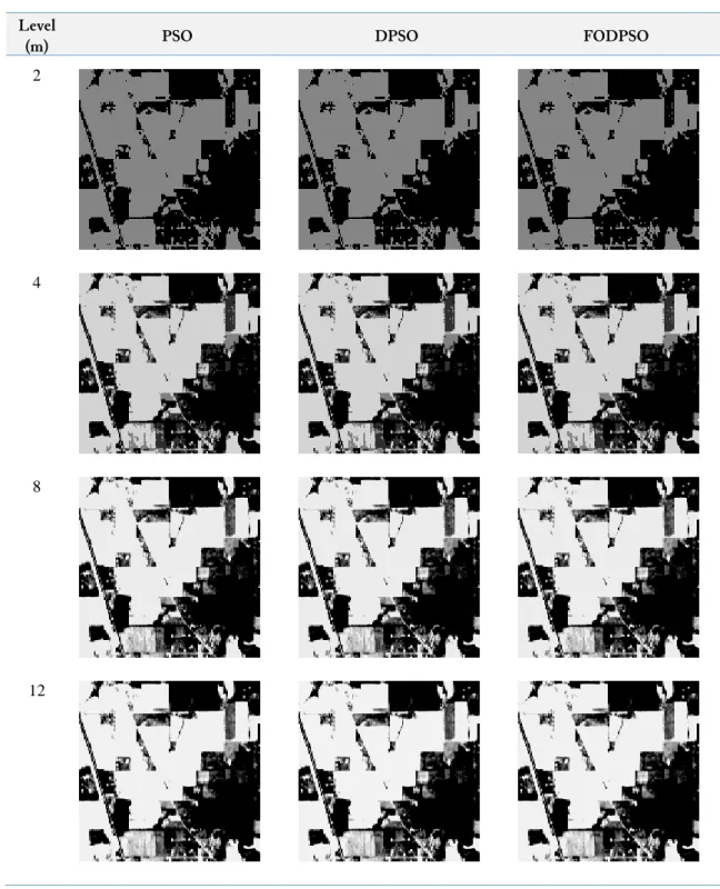
CPU processing time of the dataset used in this experiment was tested on the PSO and DPSO, FODPSO algorithms respectively for thresholding levels of 2, 4, 8 and 12. Average CPU processing time was obtained from 20 runs can be seen in Table 3. Table 4 shows results of Aviris Indian Pines image segmentation based on multi-level thresholding using swarm optimization techniques including PSO, DPSO, and FODPSO.
Table 3. Average CPU Processing Time PSO, DPSO and FODPSO
Level (m) DPSO PSO FODPSO
2 2.5228 2.8200 1.0950
4 2.8900 3.1010 2.0010
8 9.9800 10.7517 5.5246
12 12.8565 13.1281 5.8265
In Table 3, it can be seen that the CPU processing time for FODPSO is smaller than the other two methods, PSO and DPSO. At level m = 2 processing time for PSO, DPSO and FODPSO methods are 2.8200 seconds, 2.5228 and 1.0950 seconds respectively. In summary, at all levels, the FODPSO process time is the lowest compared to the others.
Table 4. Results of Multi-level Thresholding for Image Aviris Indian Pines Segmentation Using PSO, DPSO, and FODPSO
Level
(m) PSO DPSO FODPSO
2
4
8
12
4.
Conclusion
From the results of the experiment and evaluation of the research, it can be concluded that ICA technique and swarm optimizations has been implemented on the dataset of RGB images and hyperspectral images. Image segmentation is done using the particle swarm optimization (PSO), Darwinian particle swarm optimization (DPSO) and fractional order Darwinian particle swarm optimization (FODPSO). The experimental results show that FODPSO is better than PSO and DOPSO in the context of fitness value and processing time of CPU.
Acknowledgment
This research is funded by The Research Institution of Universitas Ahmad Dahlan through the Competitive Research Grant scheme in 2018 with contract number: PHB-197/LPP-UAD/III/2018.
References
[1] J. A. Richards, “Analysis of remotely sensed data: the formative decades and the future,” IEEE Trans. Geosci. Remote Sens., vol. 43, no. 3, pp. 422–432, Mar. 2005, doi: 10.1109/TGRS.2004.837326.
[2] C. M. Bishop, Pattern recognition and machine learning. springer, 2006, available at: Google Scholar. [3] Murinto and N. R. Dyah, “Feature reduction using the minimum noise fraction and principal component
analysis transforms for improving the classification of hyperspectral images,” Asia-Pacific J. Sci. Technol., vol. 22, no. 1, 2017, doi: 10.14456/apst.2017.5.
[4] R. O. Duda, P. E. Hart, and D. G. Stork, Pattern classification. John Wiley & Sons, 2012, available at: Google Scholar.
[5] A. Hyvärinen, J. Karhunen, and E. Oja, Independent Component Analysis, 2001, doi: 10.1002/0471221317. [6] Murinto and A. Harjoko, “Dataset feature reduction using independent component analysis with contrast
function of particle swarm optimization on hyperspectral image classification,” in 2016 2nd International Conference on Science in Information Technology (ICSITech), 2016, pp. 285–290, doi:
10.1109/ICSITech.2016.7852649.
[7] N. Falco, L. Bruzzone, and J. A. Benediktsson, “An ICA based approach to hyperspectral image feature reduction,” in 2014 IEEE Geoscience and Remote Sensing Symposium, 2014, pp. 3470–3473, doi:
10.1109/IGARSS.2014.6947229.
[8] C. S. Dhir, J. Lee, and S.-Y. Lee, “Extraction of independent discriminant features for data with asymmetric distribution,” Knowl. Inf. Syst., vol. 30, no. 2, pp. 359–375, Feb. 2012, doi: 10.1007/s10115-011-0381-9. [9] D. D. Lee and H. S. Seung, “Algorithms for Non-negative Matrix Factorization,” in Advances in Neural
Information Processing Systems 13, T. K. Leen, T. G. Dietterich, and V. Tresp, Eds. MIT Press, 2001, pp. 556–562, available at: http://papers.nips.cc/paper/1861-algorithms-for-non-negative-matrix-factorization. pdf.
[10] P. Deepa and K. Thilagavathi, “Feature extraction of hyperspectral image using principal component analysis and folded-principal component analysis,” in 2015 2nd International Conference on Electronics and
Communication Systems (ICECS), 2015, pp. 656–660, doi: 10.1109/ECS.2015.7124989.
[11] K. Zhang and L.-W. Chan, “Dimension reduction as a deflation method in ICA,” IEEE Signal Process. Lett., vol. 13, no. 1, pp. 45–48, Jan. 2006, doi: 10.1109/LSP.2005.860541.
[12] U. Sakarya, “Thermal infrared hyperspectral dimension reduction experiment results for global and local information based linear discriminant analysis,” in 2015 23nd Signal Processing and Communications Applications Conference (SIU), 2015, pp. 268–271, doi: 10.1109/SIU.2015.7129811.
[13] J. Li and Y. Qian, “Dimension reduction of hyperspectral images with sparse linear discriminant analysis,” in 2011 IEEE International Geoscience and Remote Sensing Symposium, 2011, pp. 2927–2930, doi:
10.1109/IGARSS.2011.6049828.
[14] P. Ghamisi, M. S. Couceiro, N. M. F. Ferreira, and L. Kumar, “Use of Darwinian Particle Swarm Optimization technique for the segmentation of Remote Sensing images,” in 2012 IEEE International Geoscience and Remote Sensing Symposium, 2012, pp. 4295–4298, doi: 10.1109/IGARSS.2012.6351718. [15] P. Ghamisi, M. S. Couceiro, F. M. L. Martins, and J. A. Benediktsson, “Multilevel Image Segmentation
Based on Fractional-Order Darwinian Particle Swarm Optimization,” IEEE Trans. Geosci. Remote Sens., vol. 52, no. 5, pp. 2382–2394, May 2014, doi: 10.1109/TGRS.2013.2260552.
[16] Y. Tarabalka, J. A. Benediktsson, and J. Chanussot, “Spectral–Spatial Classification of Hyperspectral Imagery Based on Partitional Clustering Techniques,” IEEE Trans. Geosci. Remote Sens., vol. 47, no. 8, pp. 2973– 2987, Aug. 2009, doi: 10.1109/TGRS.2009.2016214.
[17] R. V. Kulkarni and G. K. Venayagamoorthy, “Bio-inspired Algorithms for Autonomous Deployment and Localization of Sensor Nodes,” IEEE Trans. Syst. Man, Cybern. Part C (Applications Rev., vol. 40, no. 6, pp. 663–675, Nov. 2010, doi: 10.1109/TSMCC.2010.2049649.
[18] J. Kennedy and R. Eberhart, “Particle swarm optimization,” in Proceedings of ICNN’95 - International Conference on Neural Networks, vol. 4, pp. 1942–1948, doi: 10.1109/ICNN.1995.488968.
[19] J. Kennedy and R. C. Eberhart, “A discrete binary version of the particle swarm algorithm,” in 1997 IEEE International Conference on Systems, Man, and Cybernetics. Computational Cybernetics and Simulation, vol. 5, pp. 4104–4108, doi: 10.1109/ICSMC.1997.637339.
[20] J. Tillett, T. Rao, F. Sahin, and R. Rao, “Darwinian particle swarm optimization,” Proc. 2nd Indian Int. Conf. Artif. Intell., pp. 1474–1487, 2005, available at : https://scholarworks.rit.edu/other/574/.
[21] E. J. S. Pires, J. A. T. Machado, P. B. de Moura Oliveira, J. B. Cunha, and L. Mendes, “Particle swarm optimization with fractional-order velocity,” Nonlinear Dyn., vol. 61, no. 1–2, pp. 295–301, Jul. 2010, doi: 10.1007/s11071-009-9649-y.
[22] M. S. Couceiro, R. P. Rocha, N. M. F. Ferreira, and J. A. T. Machado, “Introducing the fractional-order Darwinian PSO,” Signal, Image Video Process., vol. 6, no. 3, pp. 343–350, Sep. 2012, doi: 10.1007/s11760-012-0316-2.
[23] K. S. Fu and J. K. Mui, “A survey on image segmentation,” Pattern Recognit., vol. 13, no. 1, pp. 3–16, Jan. 1981, doi: 10.1016/0031-3203(81)90028-5.
[24] R. H. Turi, Clustering-based colour image segmentation. Monash University PhD thesis, 2001, available at: http://users.monash.edu/~roset/thesis/thesis.pdf.
[25] N. Otsu, “A Threshold Selection Method from Gray-Level Histograms,” IEEE Trans. Syst. Man. Cybern., vol. 9, no. 1, pp. 62–66, Jan. 1979, doi: 10.1109/TSMC.1979.4310076.
[26] T. Pun, “A new method for grey-level picture thresholding using the entropy of the histogram,” Signal Processing, vol. 2, no. 3, pp. 223–237, Jul. 1980, doi: 10.1016/0165-1684(80)90020-1.
[27] M. S. Couceiro, R. P. Rocha, and N. M. F. Ferreira, “Ensuring ad hoc connectivity in distributed search with Robotic Darwinian Particle Swarms,” in 2011 IEEE International Symposium on Safety, Security, and Rescue Robotics, 2011, pp. 284–289, doi: 10.1109/SSRR.2011.6106752.
[28] C. Ece and M. M. U. Mullana, “Image quality assessment techniques pn spatial domain,” IJCST, vol. 2, no. 3, 2011, available at : http://citeseerx.ist.psu.edu/viewdoc/download?doi=10.1.1.219.5535&rep=rep1&type= pdf.
[29] A. Darwish, K. Leukert, and W. Reinhardt, “Image segmentation for the purpose of object-based classification,” in IGARSS 2003. 2003 IEEE International Geoscience and Remote Sensing Symposium. Proceedings (IEEE Cat. No. 03CH37477), 2003, vol. 3, pp. 2039–2041, doi: 10.1109/IGARSS.2003.1294332. [30] Murinto, S. Winiarti, D. P. Ismi, and A. Prahara, “Image enhancement using piecewise linear contrast stretch methods based on unsharp masking algorithms for leather image processing,” in 2017 3rd International conference on science in information technology (ICSITech), 2017, pp. 669–673, doi:
10.1109/ICSITech.2017.8257197.
[31] A. M. Eskicioglu and P. S. Fisher, “Image quality measures and their performance,” IEEE Trans. Commun., vol. 43, no. 12, pp. 2959–2965, 1995, doi: 10.1109/26.477498.
[32] B. Akay, “A study on particle swarm optimization and artificial bee colony algorithms for multilevel thresholding,” Appl. Soft Comput., vol. 13, no. 6, pp. 3066–3091, Jun. 2013, doi: 10.1016/j.asoc.2012.03.072.