The implementation of a dual monetary system in Indonesia

International Journal of Economics and Business Administration Volume VIII, Issue 3, 2020

pp. 28-39

The Implementation of a Dual Monetary System

in Indonesia

Submitted 14/05/19, 1st revision 09/06/20, 2nd revision 01/07/20, accepted 20/07/20

Imamudin Yuliadi

Abstract:

Purpose: This study explains the economic implications of the implementation of a dual monetary system in Indonesia's macroeconomic performance. The research is essential to know the difference between the influence of Islamic monetary system and conventional monetary system in influencing Indonesia's macroeconomic performance.

Design/Methodology/Approach: The research model is a vector autoregressive (VAR) to explain the impact of monetary on real economic performance. The variables used in this study were GDP, money supply (M2), core money (Mo), BI rate, consumer price index (CPI), gold price, composite stock price index (CSPI), mudharabah profit-sharing rate, Musharaka profit-sharing rate, Indonesian production index (IPI), Jakarta Islamic Index (JII), and exchange rates.

Findings: The results of this study revealed that there were significant differences between the conventional monetary system and the Islamic monetary system in driving the economy in real terms.

Practical implications: The recommendations of this study are the need for integration and coordination in the Islamic monetary system and the conventional monetary system to improve monetary transmission mechanisms in the real sector.

Originality/Value: The study analyzes the implications of a dual monetary system implementation in Indonesia. Theoretically, there is a difference between the monetary transmission mechanism in the Islamic monetary system and the monetary transmission mechanism in the conventional monetary system.

Keywords: Monetary transformation, dual monetary system, monetary stability. JEL Codes: E42, E52, O23.

Paper Type: Research article.

1. Introduction

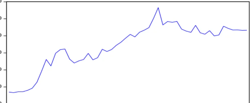
The monetary transmission mechanism in a dual monetary system is a new phenomenon of the process of transmission from the monetary sector to the real sector in the conventional monetary system and Islamic monetary system through various economic channels to achieve economic growth and desired monetary stability (Altavilla, 2019; Blanchard and Perotti, 2002; Zholud et al., 2019; Lubik and Matthes, 2016). Indonesia is a country that implements a dual monetary system, namely a conventional monetary system based on interest rates and an Islamic monetary system based on profit and loss sharing (Astiyah, 2006). The consequences of implementing a double monetary system give rise to increased complexity and increasingly diverse economic risks (Gaiotti and Secchi, 2006). Indonesia, as an open country also cannot be separated related to the dynamics of the global economy, so changes that occur in aspects of world trade and finance will have an impact on the condition of the domestic economy (Nizam, 2019). The novelty of this study concerns the implications of a dual monetary system implementation in Indonesia‘s monetary transmission mechanism (Ascarya, 2014). The development of monetary inductors of the rupiah exchange rate against the US dollar is shown in Figure 1 below.

Figure 1. Fluctuations in the Rupiah Exchange Rate against the US Dollar

9,000 10,000 11,000 12,000 13,000 14,000 15,000

I II III IV I II III IV I II III IV I II III IV I II

2013 2014 2015 2016 2017

KURS

Source: Bank Indonesia, 2018.

Theoretically, there is a difference between the monetary transmission mechanism in the Islamic monetary system and the monetary transmission mechanism in the conventional monetary system (Astiyah, 2006). The Islamic monetary system is a monetary system that does not use interest instruments but is based on profit and loss sharing and based on the underlying economic sectors (Izhar and Asutay, 2007; Hasanah, 2008). Meanwhile, the conventional monetary system based on the interest rate as an instrument for monetary transmission mechanism affects the real sector through price channels and others with all economic implications (Mishkin, 2009).

2. Literature Review

The monetary transmission mechanism in a dual monetary system can cause policy complications because there are differences in the basis of monetary instruments (Darrat, 2000; Satrya et al., 2018). The monetary transmission mechanism is a working process of monetary policy by the Central Bank that influences economic and financial performance to achieve the expected economic goals (He, 2017; Talyor, 1995; Thalassinos et al., 2015; Wildowicz-Giegiel and Kargol-Wasiluk, 2020). The effect of changes in monetary instruments on other economic indicators can be formulated in an equation, as follows (Chadha, 2009):

Yt = Et Yt + 1 – λ (Rt – Et ∏t + 1) + єA, t

Πt = β Et πt + 1 + K(Yt – ϔt) + єB, t

Mt – Pt = Yt – ηRt

Rt = ϕπ πt + єc, t

Ӯt = єd,t

The impact arising from the operation of the monetary sector to the real sector is also influenced by changes in people's behavior in responding to changes in rules and regulations so that the mechanism of monetary transmission to the real and financial sectors is characterized by aspects of uncertainty and the existence of unexpected things due to the entry of economic and non-economic factors (Brinkmeyer and Borner, 2015; Alstadheim, Bache, Holmsen, Maih, and Røisland, 2010).

3. Data and Research Methods 3.1 Unit Root Test

Research-based on time coherent data began with an explanation of how the stationarity test of the data in research with unit root tests through the Augmented-Dickey Fuller (ADF) or Philips-Perons (PP) method. The theoretical basis of the Augmented-Dickey Fuller test (ADF) can be formulated with the following format (Gujarati, 2004):

ΔYt = y1 + a2 t+ ρYt-1 +i ΔYt-1 + et

ρ = a – 1

where t is a lag based length i = 1, 2, 3, ...t

The statistical value of Augment-Dickey Fuller (ADF) is the same as the value of Dickey-Fuller (DF).

Ho: ρ = 0 (indicates the unit root). Ho is rejected if the ADF statistical value of the critical value at α or ρ value is smaller than the significance value of α.

3.2 Cointegration Test

The cointegration test was used to determine whether there were similarities in movement and long-term relationships between the variables in the study. Cointegration test was carried out using the Johansen cointegration test method, with the following format (Gujarati, 2004; Chapsa et al., 2018):

Yt = At Yt-1 + ... + Aρ Yt-ρ + B Xt + єt

Where Yt is a vector with k as a non-stationary variable, Xt is a vector with d as a

determinant variable and єt as an error vector. Cointegration test reveals that all

variables were not stationary at the level, except the gold variable, either by the Augmented-Dickey Fuller (ADF) or Philips-Perons (PP) method. Because all stationary variables were in the first difference, the model application in this study used the approach of the vector error correction model (VECM) analysis instead of VAR.

The research is a survey of the description of multiple monetary policies in Indonesia by comparing the transmission mechanism of the monetary sector to the real sector between the conventional monetary system and the Islamic monetary system. The results of the cointegration test on conventionl monetary system that with the trace value, four equations were cointegrated with a significance level of 5%. Whereas, with the maximum Eigenvalue, it can be seen that with a significance level of 5%, there were also four cointegration equations. From the cointegration test results, it is known that the movement of research variables, namely BI rate, exchange rate, CSPI, IPI, and M2, had a relationship of stability or balance and the similarity of long-term movements. The result of cointegration test in the Islamic monetary system model that included selected variables, namely M0, JII, mudharabah deposits, gold prices with trace values, there were two cointegration equations with a significance level of 5%. Whereas, with the maximum Eigenvalue, it can be seen that with a significance level of 5%, there were three cointegration equations. From the results of the cointegration test, it is known that the movement of research variables, namely M0, JII, mudharabah deposits, and gold prices, had stability or balance relationship and the similarity of long-term changes.

3.3 Determination of Optimal Lag Length

The optimal lag length based on AIC, SC, and HC criteria that indicated the optimal lag occurred in the 1st lag. Determination of the optimal lag length in the first lag would be further developed by analyzing the vector autoregressive (VAR) or vector error correction model (VECM) to find out how the correlation between the variables studied both in the long term and short term (Intriligator, Bodkin, and Hsiao, 1996).

Lyi = yt – 1 Lkyi = yt – k Lk + s = LkLs = LsLk L0 = 1, so that L0yi = yi

cL = Lc (a + b)L = aL + bL (ab)L = a(bL) L(c + v) = Lc + Lv 3.4 VAR Stability Test

VAR stability test was needed before further analysis was done, including analysis of impulse response function (IRF) and forecast error variance decomposition (FEVD) analysis. A VAR system is said to be stable if the value of all its roots has a modulus of less than one. The results of the VAR stability test using the autoregressive (AR) roots, there was a VAR/VECM analysis model stability. Also, it means that the conventional monetary system and Islamic monetary system model could be continued with the next analysis stage, namely VAR or VECM estimation for analysis of impulse response function (IRF) and forecast error variance decomposition (FEVD) analysis (Maier, 2010).

4. Results and Discussion

4.1 Islamic Monetary System Transmission Mechanism

In the Islamic monetary system in this study, the monetary variable was determined by the variables of JII, M0, mudharabah deposit profit sharing, and the price of gold. Meanwhile, the real sector variable was indicated by the IPI variable, and the following is the estimation results using the VAR method (Table 1):

Table 1. Estimation of the VAR Model of the Islamic Monetary System

IPI MO PLS_MUDH JII GOLD

IPI(-1) 0.550053 3155.876 -0.220826 0.088981 -5.177487 (0.14419) (1713.48) (0.09188) (1.42584) (3.34399) [ 3.81487] [ 1.84179] [-2.40353] [ 0.06241] [-1.54830] IPI(-2) -0.105119 2711.318 0.016719 1.938371 -1.279578 (0.16992) (2019.25) (0.10827) (1.68027) (3.94071) [-0.61865] [ 1.34273] [ 0.15442] [ 1.15361] [-0.32471] MO(-1) 1.22E-05 0.332951 1.56E-05 7.93E-05 0.000118 (1.3E-05) (0.15745) (8.4E-06) (0.00013) (0.00031) [ 0.92191] [ 2.11460] [ 1.85286] [ 0.60553] [ 0.38301] MO(-2) 3.83E-05 0.107671 -4.46E-06 7.68E-05 2.20E-05

(1.2E-05) (0.14598) (7.8E-06) (0.00012) (0.00028) [ 3.11440] [ 0.73755] [-0.56935] [ 0.63226] [ 0.07711] PLS_MUDH(-1) 0.009194 1767.687 0.807108 1.167869 3.257134 (0.25285) (3004.77) (0.16111) (2.50035) (5.86402) [ 0.03636] [ 0.58829] [ 5.00954] [ 0.46708] [ 0.55544] PLS_MUDH(-2) -0.191908 619.9587 -0.181479 0.934589 -4.173367 (0.23900) (2840.18) (0.15229) (2.36339) (5.54281) [-0.80298] [ 0.21828] [-1.19168] [ 0.39544] [-0.75293] JII(-1) -0.004962 -307.4058 0.008106 0.767926 -0.218577 (0.01613) (191.714) (0.01028) (0.15953) (0.37414) [-0.30757] [-1.60346] [ 0.78856] [ 4.81366] [-0.58421] JII(-2) 0.002072 355.4347 -0.007233 -0.011759 0.031845 (0.01547) (183.862) (0.00986) (0.15300) (0.35882) [ 0.13390] [ 1.93316] [-0.73370] [-0.07686] [ 0.08875] GOLD(-1) -0.008264 -106.4575 0.000286 0.111266 0.546342 (0.00686) (81.4736) (0.00437) (0.06780) (0.15900) [-1.20532] [-1.30665] [ 0.06548] [ 1.64118] [ 3.43608] GOLD(-2) 0.017209 29.23605 0.001437 0.045357 0.077376 (0.00672) (79.8954) (0.00428) (0.06648) (0.15592) [ 2.55970] [ 0.36593] [ 0.33551] [ 0.68224] [ 0.49625] C 20.21572 -217202.0 18.31612 -440.0826 1263.974 (17.8769) (212446.) (11.3912) (176.782) (414.602) [ 1.13083] [-1.02239] [ 1.60792] [-2.48942] [ 3.04864] R-squared 0.902657 0.913028 0.715057 0.809093 0.823790 Adj. R-squared 0.877697 0.890728 0.641995 0.760143 0.778607 Sum sq. resids 236.2557 3.34E+10 95.92620 23103.18 127075.5 S.E. equation 2.461268 29249.23 1.568326 24.33905 57.08192 F-statistic 36.16455 40.94208 9.786950 16.52880 18.23263

Source:Author’scalculations.

From Table 1, it can be seen that there were only variables that significantly influenced the IPI variable, namely the amount of core money (M0) in the second lag and the price of gold in the second lag at the significance value (α) of 5%. Whereas, the other independent variables, JII, and mudharabah profit-sharing deposit showed no significant value. The magnitude of the regression coefficient of variable M0 at the second lag of 0.0000383 means that if the amount of core money increases by 1 billion rupiahs, it will increase the IPI value by 0.0000383 points. Meanwhile, the regression coefficient value of the gold price variable at the second lag of 0.0172 means that if the gold price rises by one point, it will increase the IPI index by 0.0172 points. The analysis of the transmission model in the Islamic monetary system, it is known that what influenced the IPI real sector variable was the IPI variable in the first and third lags, the second core money (M0) lag, the third lag of Jakarta Islamic Index (JII), and the second lag of gold price. With different lag lengths, it is known that more and more variables affected performance in the real sector. The coefficient value of the two lag M0 variable was 0.000043, meaning that a change in the core money amounting to 1 billion rupiahs will affect the real sector index of the IPI in the second lag of 0.000043. The coefficient value of the third lag

JII variable was 0.059, which means that an increase in the third lag JII index by one will increase the IPI index by 0.059. Meanwhile, the second lag variable of the gold price coefficient was 0.0248, indicating that an increase in gold prices of 1 million will raise the IPI index by 0.0248. This information shows that in the Islamic monetary system changes in monetary sector variables will impact the real sector after a period of time (Ifada, Faisal, Ghozali, and Udin, 2019; Ascarya, 2014). 4.2 Conventional Monetary System Transmission Mechanisms

To see how the influence of conventional monetary system transmission mechanism in moving the real sector, this study employed monetary sector variables, including the money supply in the broad sense (M2), the Composite Stock Price Index (CSPI), the Rupiah exchange rate against the US dollar (Exchange Rate), and the level BI interest (BI Rate) (Mishkin, 2009; Christensen et al., 2016; Gali, 2008). The following Table 2 reveals the estimation results of the conventional monetary system by using the second lag:

Table 2. Estimation of the VAR Model of Conventional Monetary Systems

IPI LOGIHSQ LOGKURS LOGM2 BIRATE IPI(-1) 0.467257 -0.000647 -0.002666 0.000545 -0.004386 (0.20262) (0.00313) (0.00217) (0.00095) (0.01846) [ 2.30612] [-0.20634] [-1.22663] [ 0.57190] [-0.23768] IPI(-2) -0.584329 0.007254 -0.001723 -0.000418 -0.008579 (0.21438) (0.00332) (0.00230) (0.00101) (0.01953) [-2.72567] [ 2.18767] [-0.74929] [-0.41515] [-0.43934] IPI(-3) 0.096094 -0.005785 0.002985 0.000299 -0.016795 (0.22536) (0.00349) (0.00242) (0.00106) (0.02053) [ 0.42640] [-1.65971] [ 1.23483] [ 0.28208] [-0.81820] IPI(-4) -0.329833 0.005014 -0.002341 -0.000717 0.004890 (0.20678) (0.00320) (0.00222) (0.00097) (0.01883) [-1.59512] [ 1.56766] [-1.05524] [-0.73774] [ 0.25963] LOGIHSQ(-1) 1.815869 1.253507 -0.351737 -0.036378 -1.380014 (15.7951) (0.24430) (0.16945) (0.07423) (1.43868) [ 0.11496] [ 5.13110] [-2.07570] [-0.49005] [-0.95923] LOGIHSQ(-2) -27.53785 0.053019 0.289567 0.086136 0.435630 (20.1057) (0.31097) (0.21570) (0.09449) (1.83130) [-1.36965] [ 0.17050] [ 1.34245] [ 0.91157] [ 0.23788] LOGIHSQ(-3) 32.74655 -0.277935 -0.077409 -0.037977 -0.197909 (21.6428) (0.33474) (0.23219) (0.10172) (1.97131) [ 1.51305] [-0.83030] [-0.33339] [-0.37336] [-0.10039] LOGIHSQ(-4) -24.25755 -0.158983 0.086790 -0.000651 2.176620 (16.5673) (0.25624) (0.17774) (0.07786) (1.50901) [-1.46418] [-0.62044] [ 0.48830] [-0.00836] [ 1.44241] LOGKURS(-1) 8.488181 0.470976 0.261725 0.073329 -1.934994 (23.4248) (0.36230) (0.25131) (0.11009) (2.13362) [ 0.36236] [ 1.29995] [ 1.04145] [ 0.66608] [-0.90690] LOGKURS(-2) -53.37038 -0.005356 0.185994 -0.259263 2.048942 (24.2608) (0.37523) (0.26028) (0.11402) (2.20977)

[-2.19986] [-0.01427] [ 0.71460] [-2.27385] [ 0.92722] LOGKURS(-3) 13.44807 -0.389310 0.037034 0.091043 -0.419801 (28.9961) (0.44847) (0.31108) (0.13627) (2.64108) [ 0.46379] [-0.86808] [ 0.11905] [ 0.66809] [-0.15895] LOGKURS(-4) -16.08110 0.290393 -0.250760 -0.027000 1.107968 (22.6221) (0.34989) (0.24270) (0.10632) (2.06051) [-0.71086] [ 0.82996] [-1.03322] [-0.25395] [ 0.53772] LOGM2(-1) -30.45421 -0.132380 0.253218 0.500831 0.427358 (49.7483) (0.76944) (0.53372) (0.23380) (4.53127) [-0.61217] [-0.17205] [ 0.47444] [ 2.14209] [ 0.09431] LOGM2(-2) 111.9617 0.131491 -0.118610 0.301695 -6.185254 (48.4033) (0.74863) (0.51929) (0.22748) (4.40876) [ 2.31310] [ 0.17564] [-0.22841] [ 1.32623] [-1.40295] LOGM2(-3) 3.257845 0.756597 -0.232796 0.166151 3.893699 (46.2383) (0.71515) (0.49606) (0.21731) (4.21157) [ 0.07046] [ 1.05795] [-0.46929] [ 0.76459] [ 0.92452] LOGM2(-4) 32.15012 -1.199816 0.892281 0.132530 0.863638 (42.6474) (0.65961) (0.45753) (0.20043) (3.88449) [ 0.75386] [-1.81897] [ 1.95019] [ 0.66122] [ 0.22233] BIRATE(-1) 2.189007 0.027886 0.016353 0.013143 0.864549 (2.23849) (0.03462) (0.02402) (0.01052) (0.20389) [ 0.97789] [ 0.80544] [ 0.68096] [ 1.24932] [ 4.24027] BIRATE(-2) -4.231433 0.013366 0.011178 -0.012414 0.206925 (3.01913) (0.04670) (0.03239) (0.01419) (0.27499) [-1.40154] [ 0.28624] [ 0.34511] [-0.87488] [ 0.75247] BIRATE(-3) 4.741247 -0.051202 -0.012538 -0.001212 -0.251366 (3.07579) (0.04757) (0.03300) (0.01446) (0.28015) [ 1.54147] [-1.07632] [-0.37995] [-0.08382] [-0.89724] BIRATE(-4) -1.398496 -0.000461 0.009858 0.005141 0.091643 (2.30276) (0.03562) (0.02470) (0.01082) (0.20974) [-0.60731] [-0.01295] [ 0.39904] [ 0.47503] [ 0.43693] C -1027.463 3.754521 -4.114589 -0.467815 2.645755 (285.785) (4.42012) (3.06599) (1.34312) (26.0304) [-3.59523] [ 0.84942] [-1.34201] [-0.34831] [ 0.10164] R-squared 0.935502 0.890830 0.957594 0.995232 0.977720 Adj. R-squared 0.887726 0.809963 0.926182 0.991700 0.961216 Sum sq. resids 140.0671 0.033506 0.016121 0.003094 1.162034 S.E. equation 2.277646 0.035227 0.024435 0.010704 0.207457 F-statistic 19.58102 11.01602 30.48484 281.7971 59.24132

Source: Author’s calculations.

From the VAR analysis in Table 2, it can be seen that in the conventional monetary system applying a lag length of four; it was found that the monetary variables of CSPI, M2, Exchange, BI Rate, which affected changes in the value of the real IPI variable, turned out to be only M2 and Exchange variables; while, the other variables of IHSG and The BI Rate had no significant effect in driving the real sector variables (Zholud et al., 2019; Brinkmeyer and Borner, 2015). The variable regression coefficient of the money supply in the broad sense (M2) in lag two was 111.96,

meaning that if the money supply in the broad sense (M2) rises by 1 billion rupiahs, it will increase the IPI index by 111.96. When compared to the Islamic monetary system that applied the amount of core money (M0) at the length of lag two, it was 0.000034, indicating that the effect of changes in the money supply in a broad sense (M2) was higher than the impact of changes in the amount of core money (M0). Meanwhile, the effect of the exchange rate variable on the IPI variable was -53.37, which means that if the exchange rate of the US dollar rises by 1 rupiah per US dollar (depreciation), it will reduce the IPI index by 53.37. On the other hand, the depreciation of the rupiah against the US dollar will also cause an increase in Indonesia's foreign debt burden so that it will reduce fiscal capacity in driving the real sector (Blanchard and Perotti, 2002; Mishkin, 2009). The magnitude of the coefficient of determination (R2) was 0.887, which indicates that a change in the magnitude of the independent variables simultaneously would be able to affect the change in the dependent variable by 88.7%, while the remaining 11.30% was influenced by other variables outside the model. Whereas, the coefficient of determination (R2) in the Islamic monetary system with the same format of 0.879 means that the change in the independent variable simultaneously would affect changes in the dependent variable by 87.90%, while other variables outside the model influenced the remaining 12.10%. Thus, the conclusion is that the model applied had no significant difference between that applied to the Islamic monetary system and applied to the conventional monetary system (Izhar and Austay, 2007; Hasanah, 2008).

4.3 Analysis of Impulse Response Function (IRF)

The difference in response in the long run between the Islamic monetary system and the conventional monetary system can be known from the response analysis, as shown in Figure 2:

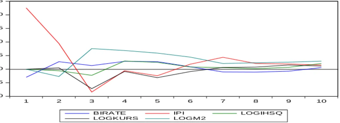
Figure 2. Analysis of Impulse Response Function in Conventional Systems

-1.0 -0.5 0.0 0.5 1.0 1.5 2.0 2.5 1 2 3 4 5 6 7 8 9 10

B IRA TE IPI LOGIHS Q

LOGK URS LOGM2

Response of IPI to Cholesky One S.D. Innovations

Figure 2 presents the analysis of responses to the conventional monetary system included exchange rates, M2, BI Rate, and IHSG, and how they responded to IPI variables. From this view, it can be seen that changes in the BI Rate, Exchange Rate, M2, and IHSG variables to the IPI showed long-term stability, namely eight years or more. It means that the Indonesian economy responded positively to the performance of these conventional monetary variables to changes in the real sector in the long term. Whereas, for the Islamic monetary system that used the variables of M0, JII, Gold, and Musyarakah Deposit Profit Sharing (PLS MUSY), it can be seen in the following Figure 3:

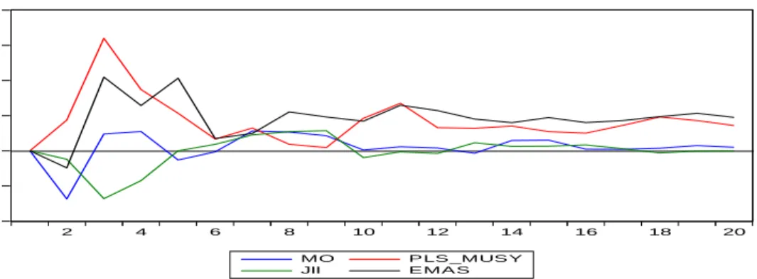
Figure 3. Analysis of Impulse Response Function of Islamic Monetary System

-0.8 -0.4 0.0 0.4 0.8 1.2 1.6 2 4 6 8 10 12 14 16 18 20 MO P LS _MUS Y JII E MA S

Response of IPI to Cholesky One S.D. Innovations

Source: Author’s calculations.

The monetary system of transmission mechanism from the monetary sector to the real sector requires a more extended period of time, namely 30 years to achieve long-term stability. It can be seen from Figure 3 above how changes in the variables of M0, Gold, JII, and PLS MUSY to the IPI variable have only reached a balance after running for 20 years. Whereas, in the conventional monetary system, long-term response stability can be achieved after running for ten years. This phenomenon is interesting because, so far, it has been claimed that the Islamic monetary system based on the real sector is considered more able to move the real sector than the conventional monetary system. It relates to infrastructure in a more mature monetary system that has more experience and reputation than the Islamic monetary system, so the conventional monetary system changes in monetary variables are relatively faster in the real sector than in the Islamic monetary system (Achasani et al., 2005; Darrat, 2000).

5. Conclusion and Recommendations

The Islamic monetary system’s transmission mechanism in moving the real sector could achieve long-term stability after more than 20 years. The conventional monetary system transmission mechanism in moving the real sector could achieve

long-term stability after running for 10 years. The recommendations of this study are as follows:

1. Improving and strengthening financial institutions and financial instruments in the Islamic monetary system encourages the effectiveness of the transmission mechanism from the monetary sector to the real sector.

2. Improvement of monetary depth and sharia financial literacy among stakeholders and the wider community further enhances the performance of sharia financial institutions as instruments to improve national economic performance and maintain national macroeconomic stability.

3. Increased cooperation with international Islamic financial institutions and business people to improve the collection of public funds and channeling the funds of Islamic financial institutions to drive the real sector productively.

References:

Ahmed Mehedi Nizam. 2019. On The Algebraic Calculation of The Fiscal Multiplier. MPRA Paper, University Library of Munich, Germany.

Alstadheim, R., Bache, I.W., Holmsen, A., Maih, J., Røisland, Ø. 2010. Monetary Policy Analysis in Practice. Staff Memo, No. 11/2010, Norges Bank, Oslo.

http://hdl.handle.net/11250/2507743.

Ascarya. 2014. Monetary Polciy Transmission Mechanism under Dual Financial System in Indonesia Interest Profit Channel. International Journal of Economics, Management and Accounting, 22(2), 1-32.

Astiyah, S., Anugrah, F.D. 2006. Integrated Monetary Policy in the Dual Banking System. Working Paper, Jakarta, Indonesia. Bureau of Economic Research, Directorate of Economic Research and Monetary Policy, Bank Indonesia.

Blanchard, O., Perotti, R. 2002. An Empirical Characterization of the Dynamic Effects of Changes in Governments Tax on Output. MIT Press, The Quarterly Journal of Economics, 117(4), 1329-1368.

Brinkmeyer, H., Borner, C.J. 2015. Drivers of Bank Landing New Evidence from the Crisis. Springer Nature Switzerland AG: Gabler Verlag. DOI: 10.1007/978-3-658-07175-2. Chadha, J.S. 2009. Monetary Policy Analysis: An Undergraduate Toolkit. Dalam G. Fontana,

M. Setterfield (Ed.), Macroeconomic Theory and Macroeconomic Pedagogy. London, Palgrave Macmillan UK, 55-75.

Chapsa, X., Tabakis, N. and Athanasenas, L.A. 2018. Investigating the Catching-Up Hypothesis Using Panel Unit Root Tests: Evidence from the PIIGS. European Research Studies Journal, 21(1), 250-271.

Christensen, L., Corrigan, P., Mendicino, C., Nishiyama, S.I. 2016. Consumption, Housing Collateral and the Canadian Business Cycle. Canadian Journal of Economics, Canadian Economics Association, 49(1), 207-236.

https://doi.org/10.1111/caje.12195

Darrat, A.F. 2000. On the Efficiency of Interest Free Monetary System: A Case Study. Paper presented in ERF's Seventh Annual Conference, Amman Jordan, 26-29 October. Gaiotti, E., Secchi, A. 2006. Is There a Cost Channel of Monetary Policy Transmission? An

Investigation into the Pricing Behaviour of 2,000 Firms. Journal of Money, Credit and Banking, 38(8), 2013-2038.

Gali, J. 2008. Monetary Policy, Inflation, and the Business Cycle: An Introduction to the New Keynessian Framework. Princeton, Princeton University Press.

He, L.T. 2017. Emphasis and effectiveness of monetary policy of the Fed: A historical comparative analysis 1871-2013. International Journal of Monetary Economics and Finance, 10(1), 47-67. https://doi.org/10.1504/IJMEF.2017.081283

Ifada, L.M., Faisal, F., Ghozali, I., Udin, U. 2019. Company attributes and firm value: Evidence from companies listed on Jakarta Islamic index. Espacios, 40(37), 11. Izhar, H., Austay, M. 2007. The Controllability and Reliability of Monetary Policy in Dual

Banking System: Evidence from Indonesia. International Islamic University Malaysia (IIUM) International Conference on Islamic Banking and Finance (IICiBF), Kuala Lumpur, Malaysia, 23-25 April.

Intriligator, M., Bodkin, R., Hsiao, C. 1996. Econometric Models, Techniques, and Applications, Second Edition. Prentice-Hall Inc, New Jersey.

Lubik, T.A., Matthes, C. 2016. Indeterminacy and learning: An analysis of monetary policy in the Great Inflation. Journal of Monetary Economics, 82, 85-106.

https://doi.org/10.1016/j.jmoneco.2016.07.006

Maier, P. 2010. How Central Banks Take Decisions: An Analysis of Monetary Policy Meetings. In P.L. Siklos, M.T. Bohl, M.E. Wohar (Ed.), Challenges in Central Banking, 320-356. Cambridge, Cambridge University Press.

Nascimento Jucá, M., Fishlow, A. 2020. Financial Crisis Effect on Latin American Companies’ Debts. European Research Studies Journal, 23(2), 421-444. DOI: 10.35808/ersj/1601.

Satrya, A., Wibowo, Ghozali, I. 2018. Does Value Creation Drives Growth Illusion? An Evidence from Indonesia Stock Exchange. European Research Studies Journal, 21(1), 491-506.

Thalassinos, I.E., Thalassinos, E.P., Venedictova, B., Yordanov, V. 2015. Currency Board Arrangement Capital Structure Macro-Financial Diagnostic. SSRN-id2624333.pdf. Wildowicz-Giegiel, A., Kargol-Wasiluk, A. 2020. The Phenomenon of Fiscal Illusion from

Theoretical and Empirical Perspective. The Case of Euro Area Countries. European Research Studies Journal, 23(2), 670-693. DOI: 10.35808/ersj/1615.