NBER WORKING PAPER SERIES
THE MARKET FOR BORROWING CORPORATE BONDS Paul Asquith Andrea S. Au Thomas R. Covert Parag A. Pathak Working Paper 16282 http://www.nber.org/papers/w16282
NATIONAL BUREAU OF ECONOMIC RESEARCH 1050 Massachusetts Avenue
Cambridge, MA 02138 August 2010
We thank seminar participants at the JACF Conference in Honor of Stew Myers, the Harvard Finance lunch, Talinn Demirjian and Jeri Seidman for comments. In addition, we are grateful to Sharat Alankar, Joseph Keith, Ted Keith, Patrick Sissman, and Caroline Hane-Weijman for research assistance. We also thank a number of practitioners for answering our questions about how this market works. Finally, we thank the Q Group for their financial support. The views and opinions expressed do not necessarily reflect those of State Street Corporation or the National Bureau of Economic Research.
NBER working papers are circulated for discussion and comment purposes. They have not been peer-reviewed or been subject to the review by the NBER Board of Directors that accompanies official NBER publications.
© 2010 by Paul Asquith, Andrea S. Au, Thomas R. Covert, and Parag A. Pathak. All rights reserved. Short sections of text, not to exceed two paragraphs, may be quoted without explicit permission provided that full credit, including © notice, is given to the source.
The Market for Borrowing Corporate Bonds
Paul Asquith, Andrea S. Au, Thomas R. Covert, and Parag A. Pathak NBER Working Paper No. 16282
August 2010 JEL No. G12,G14
ABSTRACT
This paper describes the market for borrowing corporate bonds using a comprehensive dataset from a major lender. The cost of borrowing corporate bonds is comparable to the cost of borrowing stock, between 10 and 20 basis points per year. Factors that increase borrowing costs are loan size, percentage of inventory lent, rating, and borrower identity. Trading strategies based on cost or amount of borrowing do not yield excess returns. Bonds with corresponding CDS contracts are more actively lent than those without. Finally, the 2007 Credit Crunch did not affect average borrowing cost or loan volume, but increased borrowing cost variance.
Paul Asquith
MIT Sloan School of Management 100 Main Street, E62-660
Cambridge, MA 02142 and NBER
pasquith@mit.edu Andrea S. Au
Massachusetss Institute of Technology andreau@alum.mit.edu
Thomas R. Covert Harvard Business School tcovert@hbs.edu
Parag A. Pathak
MIT Department of Economics 50 Memorial Drive
E52-391C
Cambridge, MA 02142 and NBER
1. Introduction
Short selling, where feasible, is an important activity in many asset markets. Constraints on short selling may lead to mis-valuation because they limit the ability of some market
participants to influence prices. These constraints include various institutional or legal prohibitions on taking short positions as well as the additional costs and risks associated with short selling. There is a large theoretical literature on short sale constraints and their impact on asset prices. The empirical literature on short sales, while also large, has focused almost exclusively on stocks.
In this paper, we analyze the market for borrowing and shorting corporate bonds. The corporate bond market is one of the largest over-the-counter (OTC) financial markets in the world. Between 2004 and 2007, the time period of our study, the value of outstanding corporate debt averaged slightly over $6 trillion and, according to the Securities Industry and Financial Market Association (SIFMA), trading activity averaged $17.3 billion per day.
Our analysis of shorting corporate bonds allows us to determine if the empirical findings on shorting stocks are present in other markets. In addition, unlike stocks, where borrowing takes place in an OTC market and short selling takes place on an exchange, both borrowing and shorting activities take place OTC in the corporate bond market. Thus, any effects of short sale constraints may be amplified in the bond market.
A major issue in the study of any OTC market is the availability of data. Unlike stock short positions, which are reported monthly by the stock exchanges (the NYSE reports
bi-monthly beginning September 2007), bond shorting is not regularly reported. In addition, while a number of studies have access to proprietary databases of stock lending for short periods (e.g., D’avolio 2002; Geczy, Musto, Reed 2005), comparable analyses of bond lending do not exist, with the exception of Nashikkar and Pedersen (2007).
This paper uses a large proprietary database of corporate bond loan transactions from a major depository institution for the four year period, January 1, 2004 through December 31, 2007. Although our data is only from one lender, the size and coverage of our database allows us to study the functioning of a relatively opaque, yet large market. Our lender’s par value of loanable bond inventory averages $193 billion daily and accounts for 2.9% of the overall par value of outstanding corporate bonds listed by the Fixed Income Securities Database (FISD).
From this inventory, our lender loans an average daily par value of $14.3 billion and 64.4% of bonds which appear in inventory are lent out at some point during our time period 2004-2007. Our paper uses this database to examine three primary hypotheses about the market for borrowing corporate bonds. The first is whether the market for borrowing corporate bonds has higher costs and lower liquidity than the market for borrowing stock. It does not. The borrowing costs for corporate bonds are usually low and linked to the costs of borrowing stock. In addition, we estimate that shorting represents 19.1% of corporate bond trades. The second hypothesis is whether bond shorting is motivated by investors possessing private information. The evidence is that it is not and bond short sellers do not earn excess returns on average. The third primary hypothesis we examine is whether bond borrowing activity is affected by the credit default swap (CDS) market. While it appears that bond shorting and CDS issuance are correlated, bond short selling has not been replaced by the growth of CDS.
In our database, the mean and median annual borrowing cost, equally-weighted by loan, are 33 and 18 basis points (bps) for the entire sample period. By 2007, these rates fall to 19 and 13 bps, respectively. This drop is largely because bond loans under 100 bonds have much higher borrowing costs in the early part of our sample, but are almost identical to bond loans over 100 bonds by the end of our sample. This change occurs in April 2006.
Borrowing costs are related to several factors other than loan size. Three significant factors are on-loan percentage, which is the fraction of the lender’s inventory already lent, the bond’s credit rating, and the identity of the borrowing broker. Borrowing costs remain flat until on-loan percentage reaches approximately 70% and then rise sharply. Lower rated bonds have higher borrowing costs, and borrowing costs jump at ratings downgrades and bankruptcy filings. Finally, while our lender lends to 65 brokers, a select few borrow at significantly lower rates.
We also investigate the linkage between borrowing corporate bonds and stocks. Since our lender has a significant market share of stock shorting, we construct a matched sample of corporate bonds and stock loans for the same firms. The costs of borrowing the two securities are usually quite close and 60.1% of matched loans are within 10 bps of each other. When the borrowing costs of matched loans are not close, the stock is usually more expensive to borrow than the bond.
We next study whether bond short sellers have private information. Trading strategies that short portfolios of bonds with a high on loan percentage or with high borrowing costs do not
outperform the market portfolio of corporate bonds. In addition, using the beginning and ending dates of bond loans in our database to mimic the actual positions of bond short sellers, does not generate positive excess returns.
Credit default swap (CDS) contracts provide an alternative means for investors to profit from price declines in corporate bonds. This motivates our third hypothesis of whether CDS activity impacts bond borrowing. Almost half of our shorted bonds also have CDS contracts available, but these bonds are more actively shorted than those that do not and they represent over three quarters of our loans. Moreover, borrowing costs of bonds with CDS contracts are higher than those without; one basis point higher on average and slightly more than two bps higher adjusting for cross-sectional characteristics in our regression analysis.
The Credit Crunch of 2007 began in the second half of that year. In this period, borrowing costs became more volatile, primarily because of variability in the credit market. However, the volume of bond shorting remained stable, as did the average level of borrowing costs. In addition, the average returns to shorting bonds did not change.
The remainder of the paper is organized as follows. Section 2 reviews the related
literature. Section 3 describes the mechanics of shorting a bond and estimates the market’s size. Section 4 describes our data sample, Section 5 describes the costs of borrowing, and Section 6 examines the relationship between bond and stock shorting costs. Section 7 examines the performance of bond short sellers. The next two sections consider how corporate bond shorting relates to the CDS market and whether it was impacted by the Credit Crunch of 2007. Finally, Section 10 outlines some implications of our results and concludes.
2. Related Literature
The theoretical literature on the effects of short sale constraints on asset prices is
extensive. One modeling approach examines the implications of heterogeneous investor beliefs in the presence of short sale constraints and whether this causes mis-valuation. Miller (1977) argues that short sale constraints keep more pessimistic investors from participating in the market, so market prices reflect only optimists’ valuations (see also Lintner 1971). Harrison and Kreps (1978) consider a dynamic environment and provide conditions where short sale
constraints can drive the price above the valuation of even the most optimistic investor. More recent contributions include Chen, Hong, and Stein (2002) who relate differences of opinion
between optimists and pessimists to measures of stock ownership, and Fostel and Geanokoplos (2008), who consider the additional effects of collateral constraints.
Another approach to studying the effects of short sale constraints focuses on search and bargaining frictions because investors must first locate securities to short (Duffie 1996, Duffie, Garleanu, and Pedersen 2002). Finally, there is theoretical literature in the rational expectations tradition, which examines how short sale constraints can impede the informativeness of prices (see Diamond and Verrechia 1987, and Bai, Chang, and Wang 2006).
The empirical literature on short sale constraints focuses almost entirely on stocks. An early strand of this literature examines the information content of short interest (see Asquith and Meulbroek 1995). This literature advanced in two directions as richer data sets became
available. The first direction examines daily quantities of short sales by observing transactions either from proprietary order data (Boehmer, Jones and Zhang 2008) or from Regulation SHO data (Diether, Lee, Werner, and Zhang 2009). Both papers find that short sellers possess private information and that trading strategies based on observing their trades generate abnormal returns.
The second direction in this literature examines the direct cost (or price) of borrowing stocks. These papers either use data from a unique time period when the market for borrowing stocks was public (Jones and Lamont 2002) or proprietary data from stock lenders (D’avolio 2001, Geczy, Musto, Reed 2002, and Ofek et. al 2004). Jones and Lamont (2002) and Ofek et. al. (2004) find that stocks with abnormally high rebate rates have lower subsequent returns, while Geczy et. al. (2002) find that the higher borrowing costs do not eliminate abnormal returns from various short selling strategies. D’avolio (2001) and the other three papers find that only a small number of stocks are expensive to borrow.
A challenge identified in this literature is that short interest is a quantity and borrowing costs are a price, both of which are simultaneously determined by shorting demand and the supply of shares available to short. A high borrowing cost may indicate either a high shorting demand or a limited supply of shares available to short. As a result, some researchers have constructed proxies for demand and supply and have tried to isolate shifts in either demand or supply. Asquith, Pathak, and Ritter (2005) use institutional ownership as a proxy for the supply of shares available for shorting and find that stocks that have high short interest and low levels of institutional ownership significantly underperform the market on an equally-weighted basis, but not on a value-weighted basis. Using richer, proprietary loan-level data, Cohen, Diether and
Malloy (2007) examine shifts in the demand for shorting, and find that an increase in shorting demand indicates negative abnormal returns for the stocks being shorted. Both papers highlight that their results only apply to a small fraction of outstanding stocks.
The only paper on corporate bond market shorting is Nashikkar and Pedersen (2007), who describe a proprietary dataset from a corporate bond lender between September 2005 and June 2006. Their examination of the cross-sectional determinants of borrowing costs
complements ours, although we examine additional determinants of bond borrowing costs such as borrower identity. Furthermore, our longer time period allows us to examine several time-series patterns, such as the existence and disappearance of bimodality in the distribution of borrowing costs and the 2007 Credit Crunch. Finally, we examine the profitability of short selling corporate bonds and the relationship between bond and stock shorting.
Our paper is also related to the literature which describes the transactions costs and price impact of trading corporate bonds. Bessembinder, Maxwell, and Venkataraman (2008) develop a model to test the effect of public transaction reporting on trade execution costs and Edwards, Harris, and Piwowar (2007) describe transaction costs in the corporate bond market using the TRACE dataset. That literature finds that transaction costs are higher for bonds than for stocks, but decrease significantly with trade size. It also finds bonds that are highly rated and recently issued have lower transactions costs. Using borrowing costs, not transaction costs, we find that bonds and stocks have similar borrowing costs, but that size and rating do have an effect.
3. Shorting a Corporate Bond: Mechanics and Market Size
The primary purpose of borrowing a corporate bond is to facilitate a short sale of that bond. Aside from market making activities, investors short bonds for the same reason they short stocks: to bet that the security will decline in price. Usually, these bets involve views about the particular credit quality of a corporate bond, rather than views about overall future interest rate movements. Government bonds allow an investor to take a position solely on the market
movement of interest rates, so we expect that investors who believe interest rates will rise prefer to short government bonds rather than corporate bonds. Corporate bond shorting may also be part of an arbitrage strategy involving relative mis-valuations, such as trades related to the capital structure of a particular firm or trades related to CDS-corporate bond mis-valuations. In
addition, corporate bonds may be borrowed short term to facilitate clearing of long trades in the presence of temporary frictions in the delivery process.
The mechanics of shorting corporate bonds parallel those of shorting stocks. Shorted bonds must first be located and then borrowed. The investor has three days to locate the bonds after placing a short order. Investors usually borrow bonds through an intermediary such as a depository bank. Such banks serve as custodians for financial securities and pay depositors a fee in exchange for the right to lend out securities. The borrower must post collateral of 102% of the market value of the borrowed bond, which is re-valued each day. Loans are typically
collateralized with cash although US Treasuries may also be used. In our sample, 99.6% of lent bonds are collateralized by cash. Investors subject toFederal Reserve Regulation T must post an
additional 50% in margin, a requirement that can be satisfied with any security. The loan is “on-demand” meaning that the lender of the security may recall it at any time. Hence, most loans are effectively rolled over each night, and there is very little term lending.
The fee that the borrower pays for the bond loan is expressed in terms of a rebate rate. This is the interest rate that is returned by the lender of the security for the use of the collateral. For example, if the parties agree to a bond loan fee of 20 bps, and the current market rate for collateral is 100 bps, then the lender of the corporate bond returns, or “rebates”, 80 bps back to the borrower undertaking the short position. There can be great variability in the rebate rate for the same bond even on the same day. It is even possible that the rebate rate is negative, which means the borrower receives no rebate on their collateral and has to pay the lender. Finally, if a bond makes coupon payments or has other distributions, the borrower is responsible for making these payments back to the owner of the security.
There is limited information about the size of the markets for shorting any security. For stocks, all three major stock exchanges release short interest statistics once monthly.1 Short
interest is the number of shares shorted at a particular point in time. After dividing by total number of shares outstanding, short interest is often represented as a percentage. In addition, daily stock shorting information is available from January 2005 through July 2007 when Regulation SHO was in effect. Regulation SHO required all exchanges to mark stock trades as long or short. This is no longer the case.
To estimate the size of the market for shorting stocks, most researchers first examine stock short interest statistics released by the exchanges. Asquith, Pathak, and Ritter (2005) report that in 2002 the equally-weighted average short interest for stocks is approximately 2.4%
for the NYSE and AMEX combined, and 2.5% for the NASDAQ-NMS. Using Regulation SHO data, Diether, Lee, and Werner (2007) find that short sales represent 31% of share volume for NASDAQ-listed stocks and 24% of share volume for NYSE-listed stocks in 2005. Asquith, Au, and Pathak (2006) report that short sales represent 29.8% of all stock trades on the NYSE, AMEX, and NASDAQ-NMS exchanges during the entire SHO period.2 Since bonds primarily trade OTC, comparable information on short interest does not exist and Regulation SHO did not apply.
To estimate the size of the market for shorting corporate bonds, we assume that our proprietary lender’s share of the bond shorting market is identical to their share of the stock shorting market. Asquith, Au, and Pathak (2006) report that our proprietary lender lent 16.7% of all stocks shorted on the NYSE, AMEX, and NASDAQ-NMS markets during the SHO period. From Table 1, discussed below, the average daily par value of the bonds on loan by our
proprietary lender is $14.3 billion. This measure is comparable to short interest, i.e. it is the daily average par value of bonds shorted over our sample period. If we assume that our lender
represents 16.7% of the bonds lent, then total bonds lent on an average day is $85.6 billion. This is 1.3% of the par value of the average amount of corporate bonds outstanding as reported from the FISD database discussed below. Thus, by this measure, bond shorting is approximately half as large as stock shorting.
The average daily new loan volume of our proprietary lender is $550.3 million. If we again assume our proprietary lender is responsible for the same proportion of loans to bond short sellers as they are to stock short sellers, this implies that the average daily par value of corporate bonds shorted is $3.3 billion. SIFMA reports that the average daily corporate bond trading volume for the years 2004-2007 is $17.3 billion. By this measure, bond short selling would represent 19.1% of all corporate bond trades.
Using these estimates implies that shorting corporate bonds is an important market activity. The percentage of corporate bonds shorted, 1.3%, is slightly greater than half the percentage of stocks shorted, 2.5%. Furthermore, the percentage of all daily corporate bond trades that represents short selling, 19.1%, is almost two-thirds the percentage of stock trades
2 Asquith, Oman and Safaya (2010) find for a sample of NYSE and NASDAQ stocks, that short trades are 27.9% of
that entails short selling, 29.8%. Thus, at any point in time the amount of corporate bonds shorted is large, and trading in the corporate bond market includes significant short sale activity.
4. Description of Sample
We use four separate databases, two that are commercially available and two that are proprietary, to construct the sample of corporate bonds used in this paper. All four databases cover the period from January 1, 2004 through December 31, 2007. The commercially available databases are the Trade Reporting and Compliance Engine Database (TRACE) and the Fixed Income Securities Database (FISD). The two proprietary databases are a bond inventory database and a bond loan database. These databases were provided to us by one of the world’s largest custodians of corporate bonds. The bond inventory database contains all corporate bonds
available for lending, and the companion bond loan database describes the loans made from that inventory. The bond CUSIP is used as the common variable to link these four databases.
TRACE is a database of all OTC corporate bond transactions and was first implemented on a limited basis on July 1, 2002. TRACE reports the time, price, and quantity of the bond trade, where the quantity is top-coded if the par value of the trade is $5 million or more for investment grade bonds and $1 million or more for high yield bonds. Over time, bond coverage expanded in phases, and the compliance time for reporting and dissemination of bond prices shortened. Our sample begins between Phase II and III of TRACE. Phase II was implemented on April 14, 2003, while Phase III was implemented by February 7, 2005.Phase III required reporting on almost all public corporate bond transactions.3 Since the vast majority of corporate bonds are traded over-the-counter, TRACE provides the first reliable daily pricing data for corporate bonds.
The FISD database contains detailed information on all corporate bond issues including the offering amount, issue date, maturity date, coupon rate, bond rating, whether the bond is fixed or floating rate, and whether it is issued under SEC Rule 144a. We exclude any corporate bond in the inventory file that we cannot match to FISD. In addition we also exclude all
convertibles, exchangeables, equity-linked bonds, and unit deals.
3 Phase I of TRACE covered transaction information on approximately 500 bonds. It required users to report
transaction information on covered bonds to the NASD (later changed to FINRA) within 75 minutes. Phase II of TRACE expanded coverage of bonds to approximately 4,650 bonds. On October 1, 2003 the time to report was shortened to 45 minutes. A year later, on October 1, 2004, reporting time was shortened again to 30 minutes. Finally, on July 1, 2005 the reporting time was shortened to 15 minutes. Most reported trades are immediately disseminated by FINRA.
The proprietary bond inventory database contains the number of bonds in inventory and number of bonds available to lend. From January 1, 2004 through March 30, 2005 we have end-of-the month inventory information for all bonds. The database reports daily inventory
information from April 1, 2005 to December 31, 2007. In contrast to the inventory database, the loan database is updated daily for the entire period January 1, 2004 through December 31, 2007.4 For each day, the loan database includes which bonds are lent, the size of the loan, the rebate rate paid to the borrower, and an indicator of who borrows the bond. The proprietary loan database identifies 65 unique borrowers for corporate bonds. These borrowers are primarily brokerage firms and hedge funds.
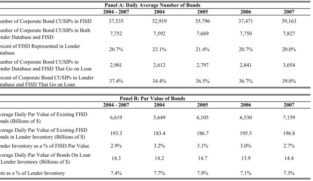
Table 1 describes the match between the proprietary bond inventory and loan databases to the overall universe of FISD corporate bonds averaged by day. Panel A shows that from 2004 to 2007, the average number of bonds in the inventory database is 7,752. This represents 20.7% of all corporate bonds in FISD for an average day. The relationship between the number of bonds in FISD and the inventory is stable over each of the four years. Although not aggregated in Table 1, there are a total of 15,493unique bonds in the bond inventory sample that match to FISD at some point. In addition, 2,901 or 37.4% of bonds in the lender inventory are on loan on an average day. There is a slight upward trend in the fraction of bonds lent from inventory during 2004 to 2007. There are 9,971 unique bonds in the merged database that are lent at some point during the four-year period.
Table 1 Panel B reports similar comparisons using the par value of the bonds. The average daily par value of corporate bonds outstanding in the FISD database during the period 2004 to 2007 is $6.6 trillion, while the average daily par value of corporate bond inventory in the database is $193 billion. This represents 2.9% of the total par value of corporate bonds issued and listed in FISD. Of this inventory, an average $14.3 billion, or 7.4% of the total par value of the inventory, is on loan each day.
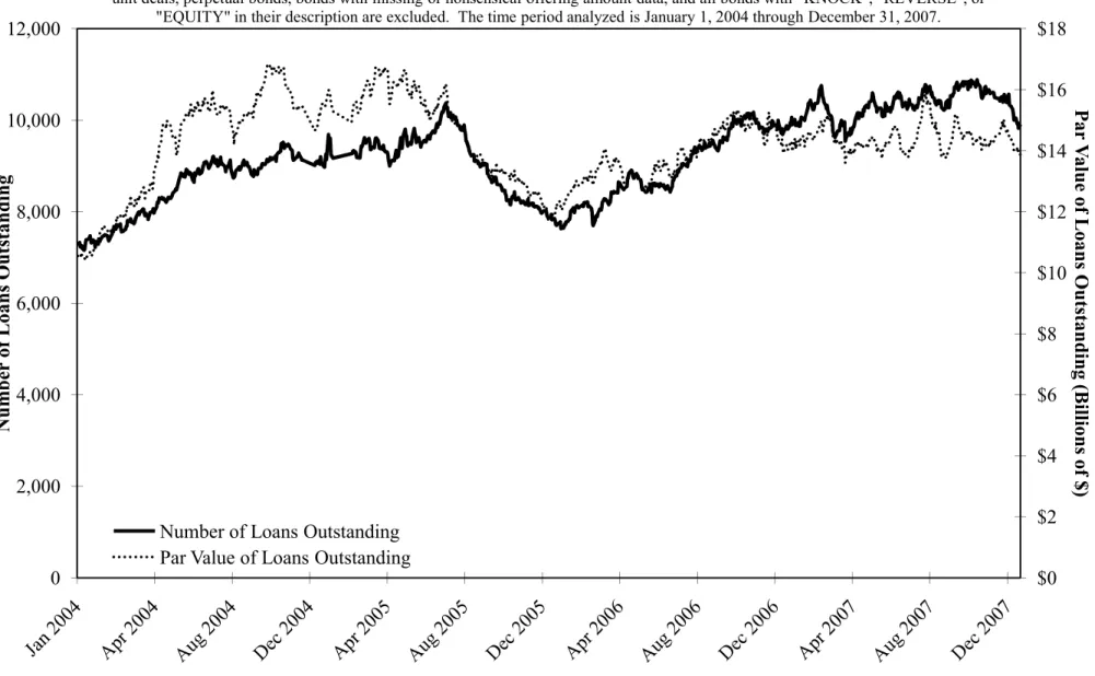
In Figure 1, we plot our proprietary lender’s number of loans outstanding, on the left hand axis, and the total par value of these loans, on the right hand axis, over time. On an average day, there are between 7,000 and 11,000 outstanding loans. The total par value of outstanding
4 There are several missing days in the loan database. On these days the file we obtained from the proprietary lender
was either unreadable or a duplicate of an earlier daily file. These days are December 16-31, 2004, all of February 2005, June 7, 2006, and November 27, 2007.
loans also fluctuates around the overall mean of $14.3 billion, with a maximum of more than $16.8 billion in October 2004, and a minimum of about $10.5 billion in January 2004.
Table 1 and Figure 1 clearly demonstrate that the number and value of corporate bonds and corporate bond loans in the two proprietary databases are large. The bond inventory database covers 20.7% of the bonds in FISD. The par value of the inventory is $193 billion on average, representing 2.9% of the $6.6 trillion market. In total, the proprietary database consists of 367,749 loans, covering 9,971 bonds, and representing an average par value of $14.3 billion per day. We believe this is of sufficient size to draw inferences about the overall market. Sample Characteristics
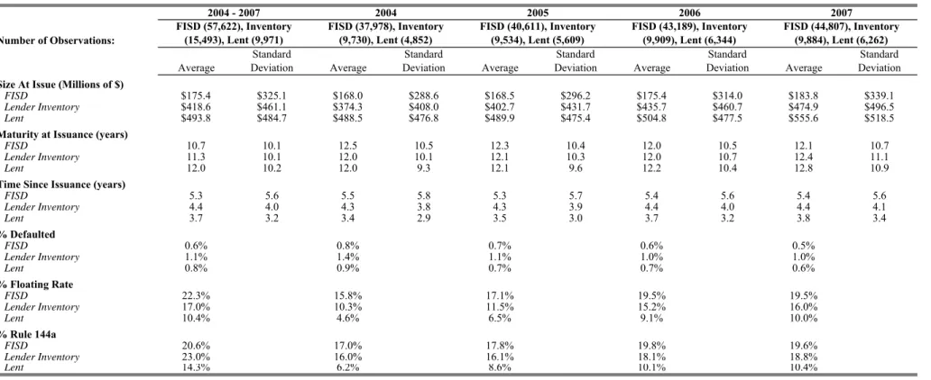
Table 2 compares various bond characteristics from FISD to the proprietary inventory and loan databases by year and for the entire period. We focus on characteristics that are likely to affect the demand and supply for corporate bond loans. The characteristics we examine are the size at issue, maturity, time since issuance, percent defaulted, percent floating rate, and percent subject to SEC Rule 144a. Rule 144a is a provision that allows for certain private resale of restricted securities to qualified institutional buyers. Table 2 allows us to determine how representative the proprietary databases are of the entire corporate bond market.
Table 2 Panel A shows that the average bond in the inventory is much larger at issue ($418.6 million) than the average FISD bond at issue ($175.4 million). The average bond lent is even larger at issue with a size of $493.8 million. The average maturity at issue of the bonds in the inventory database (10.7 years) is close to the average maturity at issue of the universe of all FISD corporate bonds (11.3 years). The average maturity at issue for lent bonds is 12.0 years. A comparison of time since issuance indicates that lent bonds are not outstanding as long as the average bond in the inventory or in FISD. There are no year-to-year trends in the values of these bond characteristics.5
Bonds in the FISD database are less likely to default (0.6%) than bonds in inventory (1.1%) and the default percentage for lent bonds is between the two (0.8%). Bonds on loan are much less likely to be floating rate bonds (10.4%) than bonds in either the FISD dataset (22.3%) or the inventory dataset (17.0%). The fraction of bonds that are subject to SEC Rule 144a is
5 The values for some of the variables, e.g. maturity and time since issuance, over the entire period are outside the
range of the per-year means. This is because each bond is only counted once for the entire period, but may be counted multiple times when counting the observations in the per-year columns. For example, the number of FISD, inventory, and lent bonds for the entire sample period is not the respective sums of the four separate years.
much higher in the FISD and inventory samples than the bonds on loan. These patterns (except for Rule 144a data) hold for the yearly comparisons as well.
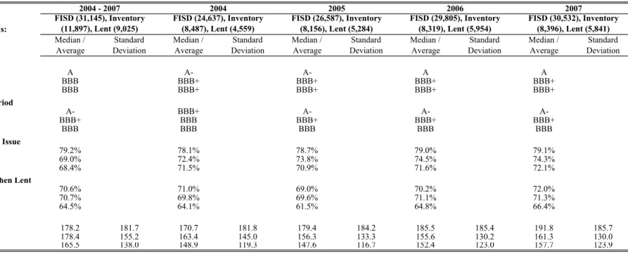
Panel B of Table 2 reports Standard and Poor’s (S&P) rating characteristics of corporate bonds. The coverage of the S&P ratings information in FISD is not as extensive as those characteristics reported in Panel A, however. For instance, there are 57,622 bonds in FISD where we observe the size at issue, while we observe S&P ratings for only 31,145 of these bonds. Fortunately, the limited coverage of ratings in FISD has a smaller impact on the
inventory and loan samples. While we have issue size information for 9,971 lent bonds, we have an S&P rating for 9,025, or 90.5% of lent bonds.
The bond inventory has a lower median rating at time of issue and over our time period than the universe of FISD corporate bonds. The sample of lent bonds has the same median rating at time of issue as inventory, but a lower rating over the entire period. The other rows of Panel B, which show percentage investment grade at issue and percentage investment grade as of the date of the loan, show a pattern consistent with the lower ratings for lent bonds than for FISD bonds.6
In summary, Table 2 shows that shorted bonds are much larger at issue, have a slightly longer maturity at issue, and have a lower median rating at issue than the average FISD bond. 69.0% of the lent bonds are investment grade, while 79.2% of all FISD bonds are. Lent bonds are also more likely to be fixed rate and less likely to be defaulted.
Properties of Short Positions
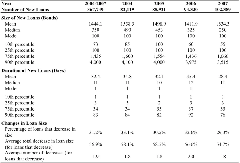
Each loan in the loan database has a unique loan number, which allows us to describe the time series properties of lent positions. Using the loan number, we are able to determine when the loan is initiated, the duration of the loan, and the number of bonds lent over the duration of the loan. Table 3 provides descriptive statistics for the new bond loans in the database for the overall period and by year. While there are 9,971 unique bonds lent in the database, there are 367,749 unique loans or an average of 36.9 loans per bond.
The data in Table 3 indicates that the size and duration of loans are skewed. The mean loan size (at par value of $1,000) is $1.44 million, but the median loan size is only $350,000.
6 The data on treasury spreads has a different pattern. The lent bonds have a smaller spread to treasuries than do our
inventory or the FISD database. It is important to note, however, that the available information on treasury spreads is much smaller than that of bond ratings, and therefore these two descriptive are not directly comparable since the samples are different. The notes in Table 2 give more information on this issue.
The mode loan size is $100,000. The mean new loan is outstanding for 32 calendar days while the median new loan is outstanding for 11 days. The mode duration of new loans is one day. There is a decrease in mean and median loan size from 2004 to 2007 (the median drops from $490,000 to $250,000). The distribution of duration of new loans is relatively stable over the four years.
The last three rows of Table 3 show how loan size changes during the life of the loan. Changes to loan size may occur if borrowers partially repay the loan or if portions of their loan are recalled by the lender. In the sample, 31.2% of loans are reduced in size before the loan is closed. Of the loans which change size, the average decrease is 56.9% of the initial loan size, and there are on average 1.9 loan decreases. We do not observe increases in loan size,
presumably because a borrower who wishes to borrow more bonds initiates a new loan. Tables 1, 2, 3 and Figure 1 show that the proprietary inventory and loan databases are extensive. The inventory database covers over 20% of all corporate bonds issued and the loan database contains over 367,000 loans on almost 10,000 bonds. The average amount in inventory per day is $193.3 billion, and the average amount on loan per day is $14.3 billion. The lent bonds are larger, have a longer duration, and have a lower rating than the average bond in the FISD database. Loan activity is large throughout the entire period. New bond loans average over $1.4 million and have an average duration of 32 days. Finally, approximately one-third of loans are partially repaid before being closed out.
5. Costs of Borrowing Corporate Bonds
The borrowing cost for corporate bonds has two major components: the rebate rate paid by the lender and the market interest rate which the borrower forgoes on the collateral. The rebate rate is the interest rate the lender pays on the collateral posted by the borrower and is typically lower than the market rate that the borrower could receive on the same funds invested at similar risk and duration elsewhere. Thus, we calculate the cost of borrowing as the difference between the market rate and the rebate rate. The loan database gives the rebate rate paid by the lender, but not the market rate. We use the one-month commercial paper rate as a proxy for the market rate.7
7 An alternative to the commercial paper rate is the Fed Funds rate. We use the commercial paper rate because we
think it more properly represents the rate the borrowers could get on their collateral. For most of the period, January 1, 2004 through December 31, 2007, the commercial paper and Fed Funds rates correlate highly (the average difference across days is 4.9 basis points and the coefficient of correlation is 0.998).
Even though most corporate bond loans are short term, as shown in Table 3, borrowing costs vary frequently over the life of the loan. Overall, 49.3% of the bond loans in the sample experience a change of at least 5 bps in their borrowing cost before repayment. These changes are due both to changes in the rebate rate and changes in the commercial paper rate. 42.3% of bond loans experience a rebate rate change of at least 5 bps, while 21.2% experience a change in the commercial paper rate of at least 5 bps.
It is possible for the lender to change the rebate rate frequently because all of the loans are demand loans. In addition, if supply and demand conditions for the bond improve, and if the lender does not lower the rebate rate, the borrower has the option of closing out the loan and borrowing from a different lender. For the loan sample, there is an average of 3.5 rebate rate changes of at least 5 bps per loan, or approximately 8 rebate rate changes for those loans with changes. Furthermore, rebate rate changes of at least 5 bps go in both directions. 38.4% of all loans have a rebate rate increase, 29.7% of all loans have a rebate rate decrease, and 25.8% of all loans have both. Hence, a considerable factor driving changes in the cost of borrowing is
changes in the rebate rate on existing loans by the lender.
The frequent changes in borrowing costs suggest that existing loans should track current market conditions, although perhaps with a lag. Comparing new and existing loans, the average absolute difference in the borrowing costs for the same bonds on the same day is 4.3 bps, with a standard deviation of 27.6 bps. Moreover, for those bonds that have new and existing loans on the same day, 46.5% of new loans have an average borrowing cost that is more expensive than existing loans and 35.4% of new loans are cheaper than existing loans. Given these differences, the analyses below only use the borrowing cost for new loans unless otherwise stated. All loans start as new loans, and new loans must reflect current market conditions.
Characteristics of Borrowing Costs
Table 4 Panel A presents the borrowing costs on new loans over time, equally-weighted by loan and value-weighted by loan size. The average borrowing cost, equally-weighted by loan (EW), is 33 bps and the median borrowing cost is 18 bps over the period 2004 to 2007. When we weight borrowing costs by the size (or par value) of the loan (VW), the mean drops to 22 bps and the median to 14 bps. This indicates that smaller loans have higher borrowing costs than larger loans. Panel A also shows that new loan borrowing costs fall substantially in 2006 and 2007. For example, the equally-weighted median borrowing costs for 2004 to 2007 are 31, 49,
16, and 13 bps, respectively. This pattern is also reflected in the mean as well as all the percentiles shown. This temporal decrease is present for both equally-weighted and value-weighted borrowing costs.
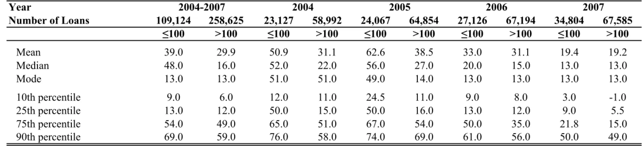
Table 4 Panel B presents borrowing costs over time partitioned by loan size. We divide loans into those of 100 bonds or less (i.e., $100,000 par value, the mode loan size) and those of more than 100 bonds. The results show that large loans have lower borrowing costs than small loans, but this difference diminishes over time. For example, in 2004 the mean borrowing cost for loans of 100 bonds or less, “small” loans, is 51 bps. For loans of more than 100 bonds, “large” loans, the mean borrowing cost is 31 bps. By 2007, the mean borrowing cost for small loans is 19 bps, which is identical to that of large loans.
Thus, Table 4 shows that on average borrowing costs fall over time, and that the
difference between equally-weighted and value-weighted borrowing costs decreases in 2006 and 2007. In addition, this decrease in borrowing cost is steeper for small loans than for large loans. Small loans are substantially more costly than large loans at the beginning of our sample period, but the costs are almost equivalent by the end of our period.
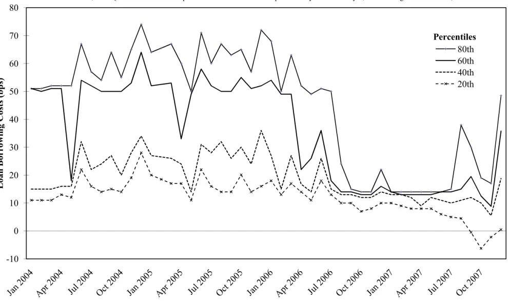
Figure 2 plots equally-weighted borrowing cost quintiles for each month of our sample period. It shows that the distribution of borrowing costs changes abruptly after March 2006. Before that date, the 60th and 80th percentiles of borrowing costs are usually at or above 50 bps for each month. After March 2006, the 60th percentile is at or below 20 bps for each month. The 80th percentile drops below 20 bps in August 2006 and is near or below 20 bps until the start of the Credit Crunch in August 2007. The plot of value-weighted loan borrowing costs, although not shown, shows a similar if less dramatic pattern during the same time period. This indicates that there was a substantial change in the pricing of bond loans in early to mid 2006 for both large and small loans.
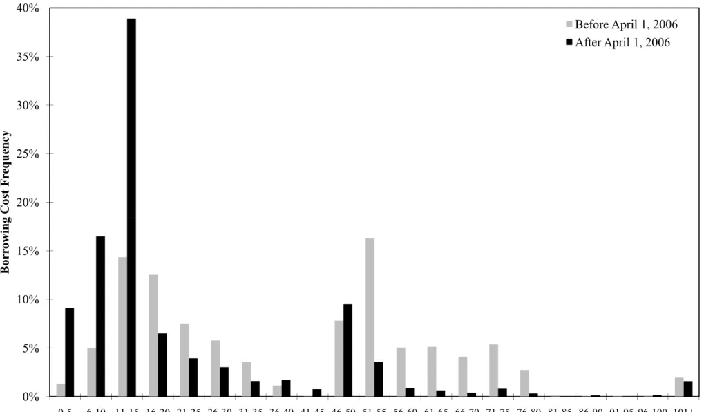
Figure 3 presents histograms of equally-weighted borrowing costs pre- and post-April 1, 2006. The lighter ‘before’ histogram shows that the most frequent borrowing cost pre-April 1, 2006 is between 51 and 55 bps, with the second most frequent borrowing cost between 11 and 15 bps. This bimodal distribution pattern is significantly changed in the darker ‘after’ histogram. The most frequent borrowing cost post-April 1, 2006 is between 11 and 15 bps, and the percentage of observations in that range is more than twice that of the highest range in the
‘before’ histogram. The range between 51 and 55 bps is now the 7th most frequent. Although not shown, the corresponding value-weighted histograms are similar.
The reasons why borrowing costs are reduced in early 2006 and why small loans began to be priced closer to large loans after that date are not immediately clear. Table 1, Table 2, and Figure 1 show that the lender’s inventory of bonds and the amount lent do not change
significantly after 2005. Further, as shown in Table 3, the average size and duration of bond loans also do not change significantly over time. Therefore, we cannot explain the change in borrowing costs with simple supply or demand proxies.
Another factor why borrowing costs change over time may be greater transparency in bond market pricing related to the growth of TRACE during our sample period. The sample begins between Phase II and III of TRACE. As stated above, Phase II was implemented on April 14, 2003, while Phase III was implemented by February 7, 2005. The last phase required
reporting on almost all public corporate bond transactions. It seems unreasonable, however, that it would take more than a year, until April 2006, for the effects of this increased coverage to have an impact. Finally, the growth of the CDS market may have driven improvements in the liquidity of corporate bonds, and the narrowing of borrowing cost spreads may reflect this trend. We investigate the impact of the CDS market for the market for borrowing corporate bonds in Section 8 below.
Determinants of Borrowing Costs
We first investigate how the cost of borrowing is related to the available supply of bonds in the lender’s inventory. As previously mentioned, we do not have daily inventory data from January 2004 to March 2005, and thus cannot compute the daily available supply of bond
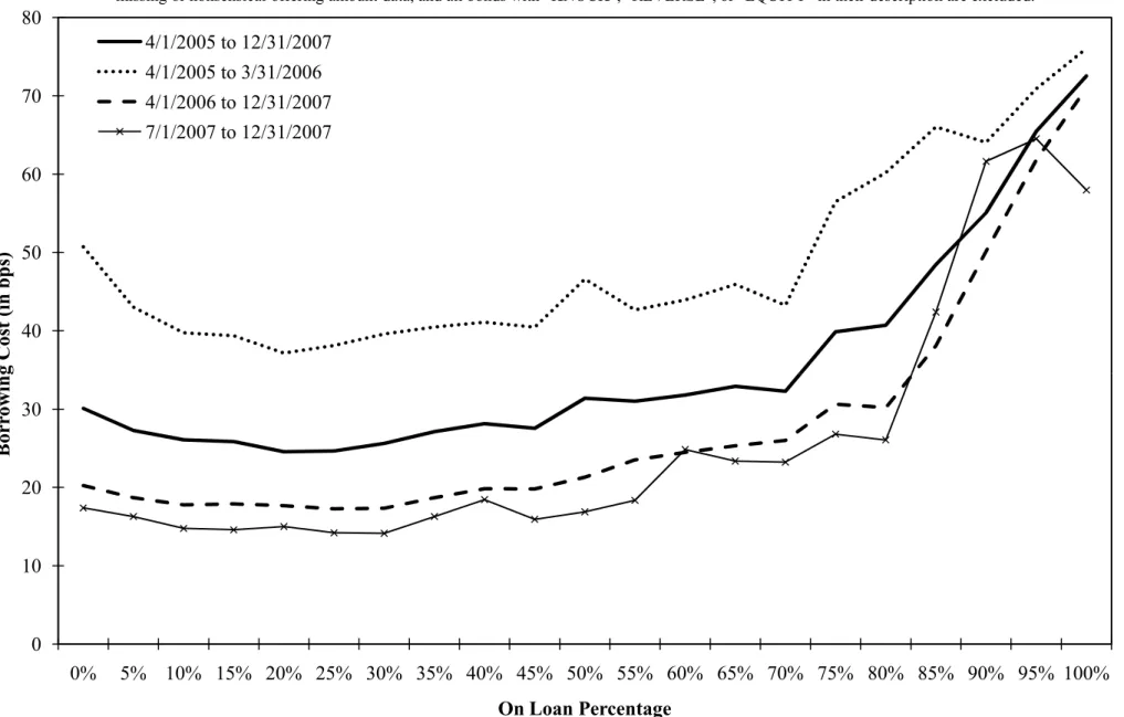
inventory during this period. Figure 4 plots the relationship between the average borrowing cost and the amount of inventory on loan for the period April 2005 to December 2007 and for several sub-periods. The vertical axis displays average borrowing cost and the horizontal axis displays amount of inventory lent. For the entire period, the average borrowing cost is relatively flat at 30 bps for bonds with less than 70% on loan. After that level, however, there is a steep increase in the average borrowing cost: each 10% increase in the amount on loan is associated with a greater than 10 basis point increase in the average borrowing cost.
Also included in Figure 4 are separate plots of average borrowing costs versus available inventory for the period April 2005 to March 2006 and for the period April 2006 until December
2007. Those two plots show that borrowing costs are significantly lower in the latter period, consistent with the results in Table 4 and Figures 2 and 3. However, a kink at 70% of available inventory still exists, and although borrowing costs are lower in the latter period, the slope of that segment is similar. This suggests that the reduction in borrowing costs in the latter half of our sample period is not due to changes in inventory. Finally, the line for the 2007 Credit Crunch is also plotted in Figure 4. We will discuss that result below in Section 9.
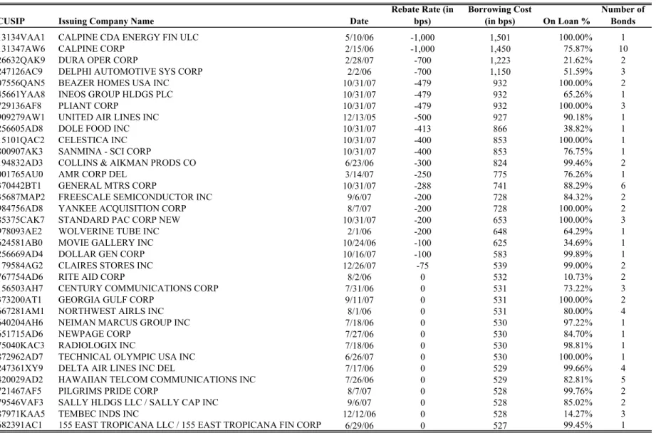
Second, Table 5 presents the 35 corporate bonds with the highest borrowing costs in the sample. Each bond is listed once, together with its maximum loan borrowing cost and the date and borrowing cost corresponding to that maximum. Since there is a great deal of clustering by firm of the most expensive bonds to borrow, the last column of Table 5 also indicates the number of bonds from that issuer where the borrowing cost is greater than the 250th most expensive to borrow bond in the sample. For example, the borrowing cost of the most expensive loan on the Calpine Corp bond with CUSIP 131347AW6 is 14.50%, but there are 10 other Calpine Corp bonds which have borrowing costs above the 250th most expensive to borrow bond in the sample.
There are three features of the bonds in Table 5 that are worth noting. First, these bonds are highly lent out. The average percentage on loan is 79.7%, well above the 70% ‘kink’ observed in Figure 4. Second, most of the firms in Table 5 experienced credit problems around the date they appeared on our list. Of the 35 firms on the list, 10 are bankrupt as of the date of the loan, while another 6, while not filing for bankruptcy, were downgraded in the year prior. In addition, 7 of the firms, while not bankrupt or downgraded, were frequently mentioned in the press in the previous year as “financially struggling.” Interestingly, 8 of the remaining firms undertook an LBO during this period. Although we didn’t check explicitly, we infer the increased leverage from the LBO impacted the bond’s borrowing cost.
A third feature of Table 5 is that a large fraction of the most expensive bond loans take place during the latter half of 2007. Thirteen out of 35 bond loans in our list are after July 1, 2007, and 8 of these are on one day, October 31, 2007. Importantly, all 8 have negative rebate rates on that date. This means their inclusion cannot be explained solely by that day’s reported commercial paper rate.
Calculated borrowing costs are not always positive. A negative borrowing cost is the result of the lender paying a rebate rate above the commercial paper rate, and it implies that the lender loses money on the loan. In total, we have 11,971 loans (or 3.3% of the total) with
negative borrowing costs in the sample. Most of the loans with negative borrowing costs
coincide with the 2007 Credit Crunch from August 2007 until December 2007. This can be seen in Figure 2, which shows that the borrowing cost of the bottom quintile becomes negative after July 2007. Of the 11,971 loans with negative borrowing costs, 8,832 of them occur between August and December 2007, of which 7,960 are on only 26 different days.
There is more than one possible reason why the cost of borrowing is negative for some bond loans. It is possible that the reported one-month commercial paper rate, which we take from the Federal Reserve Board’s website, is not representative of the true market conditions for all days. This is particularly true for those days with very large intra-day interest rate
movements. During the 2007 Credit Crunch, the Fed eased credit and dropped the Fed Funds rate several times, causing the commercial paper rate to fall as well. It is also possible that the
proprietary lender is slow to respond to changes in credit conditions.
Finally, it should be noted that during the Credit Crunch in the last half of 2007, the Fed’s intervention caused short-term rates to fall substantially below medium-term rates. If the
reinvestment rate on collateral received by the lending institution is above short-term rates, the lender can still make a profit on their bond loans even with negative borrowing costs.8
Alternatively, the Credit Crunch of 2007 may have caused borrowers of the bond to want to close out their short position and have their collateral returned. If the lender has invested the collateral in illiquid securities which have lost value, they may have difficulty in returning collateral on demand. In this instance, they may subsidize borrowers to avoid reducing their collateral pool. This scenario was reported in the financial press and a number of lenders reported losses on their collateral during this period.9 To determine if the market for lending
bonds in the period July to December 2007 is different, we examine this time period separately. We will note in Section 9 differences in any of the results for this time period.
Regression Analysis of Borrowing Costs
8 Our loan database provides a reinvestment rate which the lender estimates they will receive on the collateral. This
rate is not constant across all loans or even across all loans on one particular bond at a point in time. The reason for this is that the lender invests the collateral in a number of different funds. These funds can have a different duration and risk than that represented by investing short term at the commercial paper rate. We ignore these reinvestment rates when calculating borrowing costs since they do not represent the opportunity cost of the borrower’s collateral.
9 See Weiss, “AIG to Absorb $5 Billion Loss on Securities Lending,”
Bloomberg News, June 27, 2008 and Karmin and Scism, “Securities-Lending Sector Feels Credit Squeeze,” Wall Street Journal, October 30, 2008. Also, see State Street Press Release on July 7, 2010, “State Street Records Second-Quarter After-Tax Charge of $251 Million, or $0.50 Per Share.”
Although we know that borrowing costs are lower in 2006 and 2007 than they are in 2004 and 2005 and that borrowing costs are dependent on the size of the loan and the available
inventory to borrow, it is hard to determine the relative importance of these factors from the univariate comparisons we have made so far. We next conduct a multivariate analysis, which allows us to simultaneously control for the factors we have examined that determine a bond’s borrowing cost.
Bond characteristics may affect borrowing costs in several ways. A bond’s time since issuance may be important if it affects how widely the bond is held, and thus how difficult it is to locate, or if investor beliefs become more heterogeneous the longer the bond is outstanding. The availability to borrow may also be proxied by whether the debt is public or private (Rule 144a), as private debt may be harder to sell short. Smaller issue size may also make the bonds harder to find, increasing borrowing costs. Other bond factors that may affect borrowing costs include the bond’s rating and whether the bond is fixed or floating rate. Bonds with lower ratings might attract more loans because of their higher probability of default and thus have higher borrowing costs. Finally, the values of floating rate bonds re-price with interest rate movements and are thus less likely to deviate from par.
Borrowing costs may also differ for a given bond because of loan characteristics. A larger percentage of bonds already on loan may lead to higher borrowing costs. In addition, holding inventory constant, larger loans may have lower borrowing costs if there is a size discount. Further, borrowing costs may differ by borrower if the lender either gives a discount to large volume borrowers or if some borrowers are more knowledgeable about the lending market than others.
Our regression model incorporates the data on bond characteristics from Table 2 as well as on loan percentage, loan size, and loan initiation day dummies. In some specifications, we also include dummy variables for each bond’s CUSIP and the identity of the borrowing broker. The CUSIP controls allow us to examine how pricing varies across loan market variables, while fixing bond characteristics. Since daily inventory data is only available after March 2005, the regression analysis covers the period April 2005 through December 2007. The models we estimate are variations of the following model for the borrowing cost of loan i on bond b on day t:
β4*issue sizeb + β5*time since issuebt + β6*floating rateb + β7*rule144ab + δt + λbroker + κb + εibt,
where CPrate is the one month financial commercial paper rate (in our model 100 basis points = 1.00) and RR is the rebate rate (with the same scale as the CPrate). The on loan % is the
percentage of daily inventory already lent, and loan size is the total number of bonds lent in thousands of bonds (that is, the loan value in $ millions). Rating is the bond’s S&P rating at the time of the loan (where AAA is given a value of 1, D is given a value of 22, and all intermediate ratings are given consecutive values between 1 and 22). Issue size is the size of the initial bond offering (in $100 millions). The time since issue variable is the time since the bond was issued (in years). The floating rate variable is a dummy variable equal to 1 if the bond pays a floating rate coupon and 0 if the bond has a fixed rate coupon. The Rule 144a variable is a dummy variable equal to 1 if the bond was issued under SEC Rule 144a and 0 otherwise. δt represents a set of dummies for each trading day in the sample. κb represents a set of dummies for each bond CUSIP in the sample, and λbroker are a set of dummies for each unique borrower in the sample who borrows 100 or more times during our sample period.10 We report heteroscedasticity-robust standard errors.
Table 6 reports estimates from four specifications of the regression: one without broker or bond CUSIP dummies, one with broker dummies, one with bond CUSIP dummies, and one with both. The specifications with bond CUSIP dummies do not include issue size, time since issuance, floating rate, and Rule 144a since these characteristics are completely captured by the bond-specific and date controls.
In all four specifications the on loan % coefficient is positive and significant. In the two specifications without CUSIP dummies, the coefficient is 0.2630 without broker dummies and 0.2623 with broker dummies. When we add the bond-specific controls, the estimates fall to 0.0319 and 0.0438. The coefficients are reduced because the bond-specific controls pick up much of the variation in bond inventory. Still, consistent with the pattern we observed in Figure 4, the larger the percentage of the inventory lent, the higher the borrowing cost. Increasing the
10 Our lender identifies 65 borrowers. 40 make 100 or more loans and 25 make less than 100 loans during our
sample period. The average number of loans made by the largest 40 is 9,178 and the average made by the smallest 25 is 25. Restricting our sample to the period covered by the regression, there are a total of 62 borrowers, 38 of whom make 100 or more loans.
percentage lent by 10% is associated with an increase in borrowing costs by 2.6 bps across the sample of all bonds. For a specific bond, a 10% increase in on loan percentage is associated with an increase of 0.3 to 0.4 bps on average.
Loan size is negative and significant in each specification. Our regression results on loan size show that the larger the loan, the lower the borrowing cost. The magnitude of the
coefficient is economically large and similar across all four regression models, ranging from -0.0136 to -0.0216. This means that adding 1,000 bonds to loan size decreases borrowing costs by 1.36 to 2.16 bps.
The coefficients on bond ratings are positive and significant in all four specifications. This implies that the lower rated the bond, the higher the borrowing costs. The magnitude of the estimate is larger when we include bond-specific controls. For the specification in column (4), with broker and CUSIP dummies, the estimates imply that a full letter downgrade raises borrowing costs by 9.69 bps (three times the regression coefficient estimate of 0.0323).
The estimated coefficient for issue size is small, but positive and significant for the first two specifications. Issue size must increase by $300 million for borrowing costs to increase by 1 basis point. The coefficient on time since issuance is positive and significant in the two
specifications without CUSIP dummies, implying that the longer a bond is outstanding, the higher the borrowing cost. For every year a bond is outstanding, the borrowing cost increases by 0.7 bps.
The last two bond characteristics from Table 2 are indicators for floating rate bonds and for whether a bond is Rule 144a. The estimates imply that fixed rate bonds are almost 6 bps more expensive to borrow than floating rate bonds and that the borrowing costs for Rule 144a bonds are about 3 bps more expensive.
The identity of the borrower who initiates a loan is also important in determining borrowing costs. The proprietary database only allows us to observe the initial broker (or hedge fund); it does not allow us to determine the final party undertaking the loan transaction. In the database each bond is lent to one of 65 unique brokers who then either delivers the bonds to their own institutional and retail clients for short selling or keeps them for its own account. The specifications in Table 6 columns (2) and (4) include 38 broker dummies, each of which borrowed 100 or more bonds from April 2005 to December 2007. For both specifications, we can reject the hypothesis that all broker coefficients are zero. The difference between maximum
and minimum broker coefficients and the 75th and 25th percentile broker coefficients are also reported. In column (4), the “best” broker receives borrowing costs 59 bps less than the “worst” broker. This means that on the same day for the same CUSIP and loan size, the lowest cost broker is able to borrow at a rate 59 bps lower than the rate for the highest cost broker. This difference is considerably larger than the average borrowing cost of 33 bps as reported in Table 4. The difference between the 75th and 25th percentiles is 20 bps. Both are statistically
significant.
Table 7 further explores whether some brokers obtain lower borrowing costs. We examine all days where two or more brokers borrow the same bond. Requiring that a broker “compete” with another broker on the same day at least 100 times restricts us to consider 26 brokers. For this group, we rank each broker’s “performance” on that day for that bond by evaluating whether they received a lower, higher, or the same borrowing cost as another competing broker.11 Those results are summarized in Table 7 and show that some brokers receive consistently lower borrowing costs. We ran two sets of “competitive” races per borrower. One set was between two brokers only; the second set was between three or more brokers. The top-rated broker received the lowest borrowing cost for any given day and bond 92.5% of the time when there were two brokers and 78.9% of the time when there were three or more brokers for the same bond on the same day.
The two winning percentages of the top-rated broker are both significant using the sign test. In fact, the top eight brokers all have winning percentages which are significantly greater than 50% at the 1% level when “competing” with one other broker and significantly greater than 33% when competing with two or more brokers. Furthermore, success in the competitive races is not dependent on the number of loans or the amount borrowed by the borrower. Rank order correlations between placement in the competitive races and either the number of loans or the dollar amount of the bonds borrowed are not significant. Thus it appears that differences in borrowing costs between borrowers reflect differences in market knowledge and abilities to negotiate borrowing costs.12
11 The last line of Table 7 with Broker ID “Remainder” is a summary line that consolidates the other 39 brokers as
one competitor. The competitive race results in columns 5-8 represent contests between the combined 39 brokers and any of the 26 brokers above. It does not include contests that the 39 remaining brokers have with each other.
12 Each unique broker’s identity is available to us from the proprietary database, although we are not allowed, for
confidentiality reasons, to disclose it. The differences in borrowing costs are consistent with our perceptions of reputation.
To summarize, the borrowing cost regression results in Table 6 show that a smaller loan size, a higher percentage of inventory lent, and a lower bond rating lead to higher borrowing costs. These results hold for all four specifications of the model, although the coefficients for on loan percentage are weaker when CUSIP dummies are included. Finally, the identity of the borrowing broker significantly influences borrowing costs, both in aggregate and when comparing loans for the same bond, regardless of the broker’s volume.
Borrowing Costs Around Credit Events
We next look at borrowing costs around credit events. The events we examine are bankruptcy filings and large credit rating changes. We define a large credit rating change as a movement of three or more S&P ratings, or one full letter or more, e.g. going from an A+ to a B+ or from a BB- to an AA-. There are 241 bonds in the inventory database of corporate bonds involved in a bankruptcy, representing 93 unique bankruptcies. However, only 88 bonds have lending activity during the period from 30 trading days before until 30 trading days after the bankruptcy, which corresponds to 42 unique bankruptcies.
The average borrowing cost of these bonds for each of the 61 days is plotted in Figure 5. Since there are new loans for only 2.9 bankrupt bonds per day in the period -30 to +30 days around bankruptcy, we expand the sample by including old loans (which, as we discussed above, are re-priced). This expands the number of bonds per day in Figure 5 to an average of 60. However, each bond does not have a loan outstanding for all 61 days. We have also done the analysis only on new loans and only on bonds that have loans for all 61 days. Although there are far fewer observations, the results are qualitatively similar.
Figure 5 shows that bond borrowing costs are high for the entire period from -30 days to +30 days, where Day 0 is the bankruptcy filing date. The average equally-weighted bond borrowing cost for firms that file bankruptcy is 173 bps during the 30 days before filing. This is substantially greater than the average 33 bps reported for all new loans in Table 4 and indicates that these bonds are difficult to borrow before bankruptcy. After bankruptcy, bond borrowing costs increase further to an average of 245 bps for the 30 days after the filing. Thus, the
borrowing costs indicate that short sellers identify firms in financial distress prior to bankruptcy, but the bankruptcy filing is not completely anticipated since borrowing costs rise after that date. In Figure 6, we report a similar analysis for large bond downgrades and upgrades. There are 292 full-letter upgrade events on bonds in the inventory, covering 281 unique bonds as some
bonds have multiple upgrades. Our loan data covers 125 of these events, which correspond to 122 unique bonds. The plot for these upgrade events shows that the average upgraded bond borrowing cost is close to the average for all bonds before the upgrade and does not vary much after the rating change. The average borrowing cost for the 30 days before the upgrade is 29.9 bps, and the average borrowing cost for the 30 days after the upgrade is 32.1 bps.
The bond borrowing costs for downgrades are much lower than those for bankruptcies, but are above the average of all bonds and increase after the downgrade. There are 381 full-letter downgrade events during our time period on 356 unique bonds. The data covers 206 of these events on 193 bonds. The average borrowing cost for the bonds involved in a full-letter
downgrade is 38.4 bps in the 30 days before the downgrade and 52.3 bps in the 30 days after the downgrade. It is important to remember that all downgrades are included, including those between investment grades, i.e. from an A+ to a BBB+, and thus all downgrades do not signal financial distress.
Thus, Figures 5 and 6 show that bankruptcies and large credit downgrades increase a bond’s borrowing cost, while large credit upgrades do not decrease a bond’s borrowing cost.
6. Relationship between Bond and Stock Shorting
We next investigate how the market for shorting corporate bonds is related to the market for shorting stocks. If the purpose of borrowing securities is to short the firm, we expect the two markets to be integrated. Given the priority of claims, the stock of a firm should lose its value before the debt, suggesting that investors who wish to express a negative view about the firm may prefer to short stocks. Although investors may short debt if it is easier to access and cheaper to borrow than stock, the total market for shorting stocks is much larger than that for shorting bonds. While the proprietary lender made 367,749 bond loans over our sample period, they made 7,241,173 stock loans during the same time period.
To understand how the market for shorting corporate bonds is related to the market for shorting stocks, we matched each firm’s bonds to its corresponding common stock. We match the first 6 digits of the bond CUSIP to the first 6 digits of the common stock CUSIP. This match was not complete since many of the bonds in the dataset are subsidiaries or private firms and thus have 6 digit CUSIPs, which do not directly correspond to a common stock CUSIP. To add the subsidiary bonds (which may have a different 6 digit CUSIP), we hand matched the
we analyze our results for both methods separately, i.e. those that were matched with a 6 digit CUSIP versus those which were hand matched. There are 15,493 bond CUSIPs in the inventory file. We were able to match 5,997 using the 6-digit CUSIP match, and an additional 4,409 were matched by hand. We found no significant differences in results between the two subsamples. Another matching problem is that there are many firms with multiple bond issues. For instance, there are 124 different GM bonds in inventory, and we want to relate the borrowing costs of all of those bonds to the cost of borrowing GM’s common stock. We group all issues of bonds together for this analysis. The reason we group in this way is that for any given day, within the same firm, bondrebate rates are close. When different bonds from the same firm have a new loan on the same day, the median absolute value of the difference in bond borrowing costs is zero bps. This means that for more than half the firm-day observations, the borrowing costs are the same for all bonds of a given firm. Furthermore, the 75th percentile of this distribution is only 4 bps.
As a result, for our bond and stock analysis, if a firm has more than one new bond loan on a given day, we aggregate the borrowing costs across all bonds and all new loans by
computing value-weighted median borrowing cost. Likewise, for stocks we take the median stock borrowing cost for new loans weighted by shares lent. In our matched sample, 29.7% of new bond loans have a corresponding new stock loan on the same day.
Borrowing Costs for Matched Sample
For most firms, there is a fixed difference in borrowing cost between bond and stock loans. In particular, 76% of the firms in the matched sample have loans whose bond and stock borrowing costs differ by one of six distinct values: -10 bps, -5 bps, -1 bp, 0 bps, +35 bps, and +40 bps. This is seen in Figure 7, which plots the percentage of loans in the matched sample in each of these six categories over time.
The largest category in Figure 7 is new bond loans with borrowing costs 1 bp below new stock loans. For the matched loans, this category accounts for an average of 39.6% of
observations. This 1 bp difference is impossible to explain if bond and stock borrowing costs are not related. There are two other major fixed borrowing cost differences where bonds are cheaper to borrow than stocks. They are -5 bps and -10 bps, which average 14.0% together.
The second largest category of fixed borrowing cost differences is bond loans with borrowing costs 35 bps more expensive than stock loans. This relationship changes, however,
during our sample period. For the period from December 2004 until March 2006, the mean number of observations in this category is 22.9%. For the period from April 2006 until
December 2007, the mean number in this category is 6.8%. This drop is clearly shown in Figure 7and April 2006 appears to be a fundamental shift in the pricing relationship between bond and stock loans. Moreover, the +40 bps category, where bond loans are 40 bps more expensive than stocks, disappears by June 2006. These changes coincide with the reduction in the premium charged for small bond loans in April 2006, as described in Section 4.
There is a category that expands dramatically after March 2006: bond and stock loans that have the same borrowing cost. Before March 2006, the average percentage of matched loans in this category is 0.2%, while after March 2006, it is 7.1%. The percentage of loans in this category expands exactly when the percentage of loans in the +35 bps category decreases, although not by equal amounts. The -1 bp category also increases after March 2006.
While Figure 7 graphs the differences in bond and stock borrowing costs, it does not show their levels. This is explored in Table 8 and row 4 shows that 63.8% of loans in the matched sample have borrowing costs within 10 bps of each other. This percentage rises to 74.6% by 2007. For those matched loans whose borrowing costs are not close to one another, it is more common for the stock loan to be more expensive. In particular, only 1.2% of all matched bond loans are over 100 bps, while 6.1% of matched stock loans are over 100 bps. Furthermore, if a bond loan borrowing cost is more than 100 bps, 14.7% of matched stock loan borrowing costs also costs more than 100 bps. For the inverse, if a stock loan borrowing cost is more than 100 bps, only 3.0% of the matched bond loan borrowing costs are over 100 bps. This mean that it is more common for stocks to be hard to borrow (as measured by borrowing costs) than it is for bonds, and when a bond is harder to borrow, the stock is more likely to be as well.
To summarize, there are three main results on the relationship between bond and stock market shorting. First, most bond and stock loans for the same firm differ by one of six fixed amounts, which do not depend on the day of the loan. For example, the most common differences in borrowing costs between bonds and stocks, which are -1 bps and +35 bps, constitute 55.5% of the matched sample. Second, bond borrowing costs are very close to stock borrowing costs for most matched loans. For matched bond and stock loans from the same firm on the same day, 63.8% of the borrowing costs are within +/- 10 bps of each other, a percentage which increased to 74.6% by 2007. Finally, if neither the bond nor the stock is hard to borrow,
they are priced very similarly. However, on a day when a stock is expensive to borrow, bonds from the same firm are usually not, and vice versa. This suggests that for low levels of borrowing costs these two securities lending markets are similar, but when borrowing costs are high they are fragmented.
7. Returns to Shorting Bonds
In the last two sections, we calculated borrowing costs, described their cross-sectional and time-series distribution, and examined some of their important determining factors. In this section, we do a similar analysis on the returns to shorting bonds. As mentioned above, we do not know if all borrowed bonds are necessarily shorted, but for the purposes of this section we assume they are. The literature on stock shorting that uses proprietary lending databases makes a similar, although usually unstated, assumption. The literature on shorting stocks infers that excess returns from highly shorted stocks implies the existence of private information among short sellers and/or borrowing constraints. We make the same inference for the market for shorting bonds.
In order to calculate bond returns over any holding period, it is necessary to have bond prices at the beginning and end of the period. Following the approach of Bao and Pan (2009) we match the proprietary databases of bond inventory and loans to the FISD TRACE database, which provides transaction bond prices. The number of bonds covered in TRACE increased once during our sample period on February 7, 2005. This increase ostensibly extended TRACE’s coverage to all US corporate bonds. Even with universal TRACE coverage, there are difficulties in computing bond returns. (See Bessembinder, Maxwell, Kahle and Yu (2010) for the difficulty of working with bond returns in general and TRACE in particular.)
We calculate bond returns with the following formula:
return = (sale price – buy price + sale accrued interest – buy accrued interest + coupons paid) / (buy price + buy accrued interest).13
In this formula, the return is from the point of view of a long holder of the bond. That is, the returns are positive if the bond prices increase. A short seller of the bond, therefore, benefits if the return is negative. In the formula, sale and buy prices are “clean”, meaning net of accrued interest, which is the way prices are reported in TRACE. In some databases bond prices are
13 This is Bessembinder, Maxwell, Kahle, and Yu’s (2010) formula with a correction for a typographical error in that