Using Predictive Modeling for Cross-Program Design Space
Exploration in Multicore Systems
∗
Salman Khan, Polychronis Xekalakis
†, John Cavazos, and Marcelo Cintra
School of Informatics
University of Edinburgh
{salman.khan, p.xekalakis}@ed.ac.uk, {jcavazos, mc}@inf.ed.ac.uk
Abstract
The vast number of transistors available through modern fabrication technology gives architects an unprecedented amount of freedom in chip-multiprocessor (CMP) designs. However, such freedom translates into a design space that is impossible to fully, or even partially to any significant frac-tion, explore through detailed simulation. In this paper we propose to address this problem using predictive modeling, a well-known machine learning technique. More specifi-cally we build models that, given only a minute fraction of the design space, are able to accurately predict the behav-ior of the remaining designs orders of magnitude faster than simulating them.
In contrast to previous work, our models can predict per-formance metrics not only for unseen CMP configurations for a given application, but also for unseen configurations of a new application that was not in the set of applications used to build the model, given only a very small number of results for this new application.
We perform extensive experiments to show the efficacy of the technique for exploring the design space of CMP’s running parallel applications. The technique is used to pre-dict both energy-delay and execution time. Choosing both explicitly parallel applications and applications that are parallelized using the thread-level speculation (TLS) ap-proach, we evaluate performance on a CMP design space with about 95 million points using 18 benchmarks with up to 1000 training points each. For predicting the energy-delay metric, prediction errors for unseen configurations of the same application range from 2.4% to 4.6% and for con-figurations of new applications from 3.1% to 4.9%.
∗This work was supported in part by the EC under grant HiPEAC
IST-004408.
†The author was supported in part by a Wolfson Microelectronics
scholarship.
1 INTRODUCTION
When designing a modern chip-multiprocessor (CMP) the architect is faced with choosing the values for a myriad of system and microarchitectural parameters (e.g., number of cores, issue width of each core, cache sizes, branch pre-dictor type and size, etc.). Simulation is the tool of choice for evaluating each design point in this large design space. Unfortunately, the complexity of modern cores and CMP’s, together with the complexity of modern workloads, has in-creased the time required for accurate simulation of the de-sign space beyond practical levels.
Alternative approaches such as analytical modeling, sim-plified kernel workloads, and reduced input sets are in-creasingly undesirable as they cannot accurately capture the intricacies of realistic architectures, workloads, and input sets. Recently, statistical sampling has received much at-tention [19, 25]. These techniques have been shown to cut simulation time by 60 times in many cases with error rates of around 3%. Whether such techniques will keep pace with the increased complexity of future architectures and work-loads is an open question. In this paper we explore a differ-ent and complemdiffer-entary approach to reducing the time re-quired to explore the large design space of CMP’s running a variety of applications: predictive modeling.
Predictive modeling using statistical machine learning (e.g., regression and multilayer neural networks) has re-cently received much attention [7, 8, 11]. The key idea is to build models that once trained for a given program on a number of design points (configurations) can predict the behavior of different configurations. Constructing a model requires simulation results for only a small fraction of the entire configuration space. Both model creation and using the models to predict the performance of new configura-tions takes orders of magnitude less time than simulating these configurations. Thus, these techniques can cut down the time needed to explore a large design space by several
orders of magnitude.
Unfortunately, the simulations required for constructing predictive models are still expensive and previous work re-quires a set of simulations for every application [7, 8, 11]. In this paper, we take this technique a step further to cut down model creation time. We show that it is possible to create a model using only a subset of the applications of in-terest and then use this model to accurately predict the be-havior of new configurations for newunseenapplications. This is achieved with a technique we termreaction-based
characterization, that requires only a very small number of
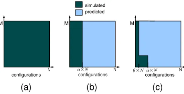
simulations for every new application not in the training set. The key intuition is that when given such a new application the model tries to automatically match this application’s be-havior against that of applications with similar bebe-havior in the training set. If such an application exists then the model can accurately predict the behavior of the new application without having to pay the cost of the model creation for the application. The idea is depicted in Figure 1. Figure 1(a) shows the case where no predictive modeling is used and the designer must simulate all the configurations for all the applications of interest. Figure 1(b) shows what happens when predictive modeling is used as in previous work. In this case, only a small fraction of the configurations must be simulated (0< α <<1) and the rest can have their be-havior predicted. Figure 1(c) shows our proposed reaction-based predictive modeling. In this case, only a subset of the applications have to be simulated for the small fraction of the configurations while the rest can have their behavior predicted after only an even smaller number of simulations
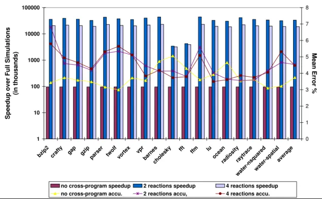
(0< β << α <<1). The benefits can be seen in Figure 2,
where the speedup in simulation time, when compared to an exhaustive simulation of the space, and accuracies are pre-sented for different predictive modeling techniques for each application. As can be seen, cross-program prediction with the reaction technique - the technique proposed in this paper - can be two to three orders of magnitude faster. Moreover, the reaction-based approach achieves these speedups while maintaining comparable accuracy.
An additional contribution of this paper is to demon-strate that this technique can be used to accurately predict not only performance but also energy-delay1(ED) results.
Energy-delay is an important metric since it is able to quan-tify whether or not a power-efficient design achieves a re-duction in the overall energy.
To evaluate our approach we use both explicitly parallel applications and applications parallelized using the thread-level speculation (TLS) approach. We show that, despite the complexity of the CMP architectures and the applications studied, we are able to perform accurate cross-program pre-dictions. Specifically, for a CMP design space with about 95M points using 18 applications with up to 1000 training
1ED = Energy * Execution Time
(a) (b) (c)
Figure 1. Fraction of the space simulated and predicted shown for (a) full simulation with no prediction (b) per program prediction and (c) cross program prediction.
points each we can predict energy-delay results with errors ranging from 3.1% to 4.9% for cross-application predic-tions, that is, training a model on a subset of applications and using the model to predict configurations for a new, un-seen application.
To summarize, the main contributions of this paper are:
• We show that highly accurate cross-application predic-tions are feasible through the use of a technique we term reaction-based modeling.
• We perform predictions of both execution time and energy-delay. We thus show that our techniques work for designs that target only performance and those that target performance within a given power envelope.
• We thoroughly evaluate our models using explicitly parallel and TLS applications. We show that our mod-els can accurately predict explicitly parallellized scien-tific applications and can predict equally well for the more complex TLS design space.
The rest of this paper is organized as follows. Section 2 presents background information and Section 3 describes our predictive model and reactions. Section 4 outlines the experimental framework and the design parameters consid-ered and Section 5 presents results. We discuss related work in Section 6 and draw some conclusions in Section 7.
2 BACKGROUND
2.1
The CMP Design Space
Chip-multiprocessors (CMP’s) offer a myriad of system-level parameters to choose from, such as the number of cores in the chip, the configuration and sizes of caches, and the number and width of memory channels etc. Addition-ally, despite the fact that focus has shifted from core design
1 10 100 1000 10000 100000 bzip 2 craf ty gap gzip pars er two lf vort ex vpr barn es chol esky fft ffm luocea n radi osity rayt race wate r-ns quar ed wate r-sp atia l aver age Sp eed u p o ver F u ll Si mu lati o n s (i n th o u s an d s) 0 1 2 3 4 5 6 7 8 M e an Er ro r %
no cross-program speedup 2 reactions speedup 4 reactions speedup no cross-program accu. 2 reactions accu, 4 reactions accu.
Figure 2. Comparison of accuracy in energy-delay prediction and speedup over simulation of the full space (in thousands).
to system design in CMP’s, these systems also offer a large number of choices of microarchitectural parameters, such as issue width, type and size of branch predictor, and number and type of functional units, just to name a few. Some of the current CMP’s also offer the possibility of multithreading, and future CMP’s are likely to offer the possibility of het-erogeneity of core types on the same chip. Overall, given the sheer number of possible CMP configurations it is in-creasingly important to be able to quickly explore the design space of these systems. Unfortunately, the subtle interac-tions among all these parameters make accurate simulation extremely expensive and make alternative approaches, such as analytical modeling, increasingly inaccurate.
2.2
Parallel Applications
Perhaps even more than sequential applications, parallel applications exhibit a great degree of variability in behavior, depending not only on the algorithm but also on the imple-mentation and the parallelization mechanism. For instance, scientific applications based on arrays and parallelized with the single program multiple data (SPMD) paradigm usu-ally have simple and predictable control and communica-tion patterns. On the other hand, parallel applicacommunica-tions writ-ten with a more general threading model writ-tend to be more
unpredictable. Unfortunately, the complex behavior of such applications make the use of alternative approaches to full simulation, such as simplified kernels and reduced input sets, also increasingly inaccurate.
For our study we chose parallel applications from two very different backgrounds. Namely, scientific applications built with explicit, shared-memory, threads (the Splash-2 suite [23]), and desktop applications written in sequential form (the SPEC int 2000 suite [21]) parallelized with the thread-level speculation (TLS) technique. Arguably, TLS applications exhibit behavior even more complex than other parallel applications, due to the possibility ofsquashes and re-execution of threads and processor stalls. For complete-ness, we present a very brief overview of the TLS technique below. Readers familiar with the technique may skip to the next section.
Under the thread-level speculation (also called
spec-ulative parallelization or speculative multithreading)
ap-proach, sequential sections of code are speculatively exe-cuted in parallel hoping not to violate any sequential se-mantics. The control flow of the sequential code imposes a total order on the threads. At any time during execu-tion, the earliest thread in program order isnon-speculative
while the others are speculative. The termspredecessor
Stores from speculative threads generate unsafeversionsof variables that are stored in some sort ofspeculative buffer, which can be simply the private caches or some additional storage dedicated to speculative parallelization. If a specu-lative thread overflows its specuspecu-lative buffer it must stall and wait to become non-speculative. Loads from speculative threads are provided with potentially incorrect versions. As execution proceeds, the system tracks memory references to identify any cross-thread data dependence violation. If a dependence violation is found, the offending thread must
besquashed, along with its successors, thus reverting the
state back to a safe position from which threads can be re-executed. In addition to this implicit memory communica-tion mechanism, some hardware environments for specula-tive parallelization allow synchronizedmemory and register
communicationbetween neighbor threads. When the
execu-tion of a non-speculative thread completes itcommitsand the values it generated can be moved to safe storage (usu-ally main memory or some shared higher-level cache). At this point its immediate successor acquires non-speculative status and is allowed to commit. When a speculative thread completes it must wait for all predecessors to commit be-fore it can commit. After committing, the processor is free to start executing a new speculative thread. Usually a pro-cessor that completes the execution of a speculative thread before the predecessor threads have committed is not al-lowed to start execution of a new speculative thread.
3 Predictive Modeling Using Reactions
3.1
Predictive Modeling
Predictive modeling describes the process of creating models that try to approximate the behavior of a system. In this black-box approach, the system can be thought of as a complex function that given some input will return some result. The set of inputs to the model is known as theinput
vectorand the behavior that has to be learned as the
tar-get function. Creating such a model is a three step process.
First, the input vectors and the target function have to be choosen. For our task, this translates to choosing the set of architecture parameters to vary that will be used as input the model (e.g., branch predictor size) and deciding on the behavior of the architecture we want to predict (e.g., energy-delay). Second, the model then has to be trained with tuples, each of which consists of an input vector and an expected output. These tuples should exhibit representative behavior, so that the model can infer accurate predictions for unseen input vectors once trained. The training algorithm depends on the target function, the type of input data, and the im-plementation of the prediction model. Third, we validate the performance of the model by feeding it previously un-seen input vectors and comparing its predicted output to the
expected output.
3.2
Reaction-based Modeling
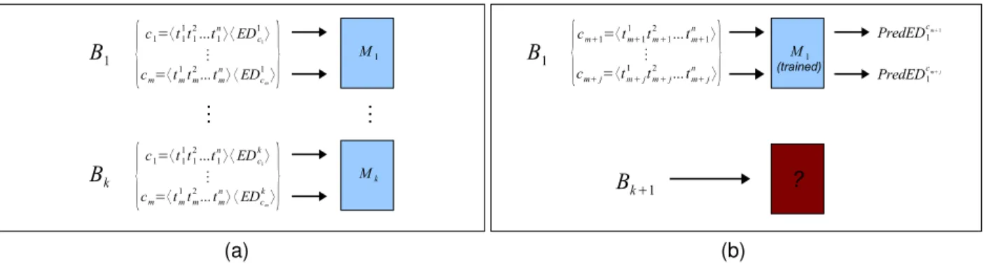
This section describesreaction-based modeling, a tech-nique for building accurate models that can predict the be-havior of unseen programs on a large set of architecture configurations simply by observing the program’s behav-ior on a very small subset of configurations chosen a pri-ori. Previous works [7, 8, 11, 12] have used automatic techniques to build predictive models. However, these tech-niques have required building a model for every new bench-mark as shown in Figure 3. As shown in this figure, in pre-vious approaches a new model is trained for every bench-mark whose behavior we want to predict. Each model is trained by feeding input vectors, each of which consists of different architecture parameters (t1throughtn) that make
up each configuration (c1throughcm) and trying to learn a
benchmark’s behavior of interest, e.g., energy-delay (EDic1
throughEDi
ck). For example, Figure 3(a) shows the
train-ing of model M1 for benchmarkB1 and model Mk for
benchmarkBk. ModelM1 can used to accurately predict
the behavior of benchmarkB1on unseen architecture con-figurations,cm+1throughcm+j, that it was not trained with.
However, we can not use any of these previously trained models to reliably predict the behavior of a new benchmark
Bk+1, as in Figure 3(b).
Figure 4 depicts our new technique which solves this problem. The approach works as follows. First, we ran-domly choose a small set of architectural configurations, we
callcanonical configurations, that will be used as a
charac-terization of a benchmark. We then obtain the energy-delay, for each benchmark in the training set on the canonical con-figurations. We call these resultsreactions. For example, in Figure 4(b) we obtain the set of reactionsR1throughRyfor
each benchmark. Suppose we use two canonical configura-tions, configurations A and B, to obtain reactions for each benchmark. The set of reactions will consist of obtaining energy-delay by running each benchmark with configura-tions A and B, giving us reactionR1 for configuration A
andR2for configuration B. Again, the reactions serve as
a characterization orsignatureof each benchmark and are used as inputs into our model along with each of the config-urations we use to train the model. The model then learns for each benchmark the metric (e.g., energy-delay) obtained when running that benchmark on each training configura-tion. Note, as depicted in Figure 4(a), that we only have to train one model now for all the benchmarks in our training set.
This model can be used to predict the performance of new unseen configurations (cm+1throughcm+j) for each
of the training benchmarks. However, the main difference between our approach and previous approaches in
perfor-(a) (b)
Figure 3. Building a predictor per program. The predictor is (a) trained and (b) probed for a prediction.
(a) (b)
Figure 4. Using reactions to do cross program prediction. The predictor is (a) trained and (b) probed for a prediction.
mance prediction is that we can use our trained model to accurately predict the performance of unseenbenchmarks
not in the training set, which we show in Figure 4(b), by predicting the behavior of benchmarkBk+1. When training
the model without using reactions, we simply use the con-figuration (t1t2...tn) as input. However, in reaction-based
modeling, we extend the input with the reactions for each canonical configuration (R1...Ry). To use the model to
pre-dict energy-delay for a new unseen benchmark, we simply need to obtain energy-delay results (reactions) for the new application by running it with the pre-determined canoni-cal configurations. These reactions are then used as inputs into the model along with the architecture configuration we want a prediction of. The intuition is, if previously studied programs had similar reactions, the new program may be classified to be similar to one or a combination of some of these previously seen programs.
This technique requiresyprogram runs for obtainingy
reactions used as input to the predictor. However, we em-pirically show in Section 5 that we can keepy very small (less than or equal to 8), and still get accurate predictions.
We formally describe the particular predictive model we chose in the next section.
3.3
Building the model using ANNs
There exist many modeling techniques that can be used to automatically produce a predictive model. In this paper we use a feed-forward ANN (Artificial Neural Network), with one hidden layer of ten units. Such an ANN is robust to noise in its input and capable of learning real-valued out-puts - both characteristics of our problem domain. ANNs are well studied and have been used in a wide range of do-mains [4] and our current experience suggests that ANNs may be practical for this prediction problem.
The model is constructed as follows: the inputs are they
reactions and the architecture configuration whose energy-delay (or performance) impact we want to predict, and the output is the predicted energy-delay (or performance) of the target configuration.
More formally, we build a modelf which takes as in-puts the reactions (e.g., energy-delay) of the program P
R1(c1;P), . . . , Ry(cy;P)toy canonical architecture
con-figurations, c1, . . . , cy, and a new architecture
configura-tion t. We use the model to predict the metric (sˆ), e.g., energy-delay, on new programs and architecture configura-tions:f(R1(c1;P), . . . , Ry(cy;P), t) = ˆs. The model can
not only be trained specific to a program, it can be trained on multiple programs, and can be applied to any unseen pro-gram thereafter, simply by running the unseen propro-gram with the canonical configurations. Figure 4 depicts the training and usage of our ANN models for both the case of using re-actions. In the figure, the superscript on each variablet cor-responds to an individual attribute (e.g., L1 DCache size) of the configuration.
The y reactions (or canonical) architecture configura-tions are chosen at random and provide a characteristization of the program behavior to be used todiscriminatebetween the training programs.
4 EVALUATION METHODOLOGY
4.1
Applications
To evaluate our techniques for predictive modeling of CMP configurations we chose parallel applications from two very different backgrounds. The first set of applica-tions are from the Splash-2 suite [23]. These are explicitly parallel, shared-memory, scientific applications and kernels written with a generic programming model based on locks and barriers. From these we did not includeradixand vol-rendbecause we could not correctly run them on our simu-lator. The second set of parallel applications are from the SPEC int 2000 suite [21], which were parallelized using the thread-level speculation (TLS) technique. From these we did not includeeonbecause it is in C++ andgcc,mcf,
andperlbmkbecause our TLS compiler infrastructure
(Sec-tion 4.2) failed to compile them.
4.2
Compilation, Simulation, and
Model-ing Environments
The SPEC int TLS applications were compiled with the POSH compiler infrastructure [13], which is based on gcc 3.5. For these applications, we exclude initialization and execute code sections that correspond to 500 million com-mitted instructions in the original sequential version (note that with TLS the same dynamic instruction may “commit” multiple times when a thread is squashed and re-executed). The reference input sets were used for these applications. The Splash-2 applications were compiled with the MIPSPro SGI compiler at the03optimization level. These applica-tions were executed to completion using the reference input sets.
For the detailed execution driven simulations we used the SESC simulator [17]. This simulator models in detail the CMP system and the internal microarchitecture of each core. The timings and power consumption estimates used by this simulator are based on CACTI 3.0 models [20]. For the TLS applications the CMP is augmented with hardware
support for TLS, which is built into SESC. This hardware support is described in [18]. For the neural network models we used Matlab and the neural network toolbox.
4.3
Learning Model
We use a standard two layer feedforward neural network for prediction. The network has hyperbolic tangent sigmoid activation for hidden layer neurons and linear activation for the output. Each configuration is presented as a 9 dimen-sional input vector to the ANN. For cross-program predic-tion, this input vector is extended with the reactions. To avoid overfitting, we use regularization using a bayesian ap-proach for parameter selection [14]. Regularization incor-porates the sum of squared weights from the network into the error function. Keeping the weight value low keeps the function that the network represents smooth and thus im-proves generalization. It has the added advantage over early stopping that we can train on all the data rather than keep-ing some for a stoppkeep-ing set. For all our predictions, we use a network with one hidden layer of 10 neurons.
4.4
Designs Evaluated
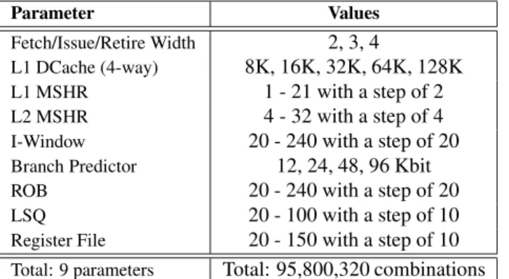
As discussed in the previous sections, we look at a CMP design space. More specifically, we look into different branch prediction sizes, issue/rename/commit widths, re-order buffer sizes, window and load-store queue size, differ-ent numbers of L1 and L2 miss handling registers (MSHR) and different register file sizes. The detailed values for the parameters we varied can be seen in Table 1. We choose not to vary the instruction cache parameters, because our appli-cations have very small instruction miss-rates and even sub-optimal configurations did not affect their performance. For the branch predictor, we used a hybrid bimodal-gshare [15], a well established and reasonably accurate predictor. Due to its fast learning component (bimodal), it is also ideal for the thread-switch behavior of TLS systems. We assume a one cycle access latency and a minimum of 11 cycles branch misprediction latency. We also employ speculative updates of the global history register similar to previous work [9]. We use a four core CMP for all our experiments. The total number of possible value combinations (design space) is in excess of 95 million.
5 EXPERIMENTAL RESULTS
We run a number of experiments to establish a base-line and evaluate the improvements in prediction accuracy achieved by using reactions. We concentrate on predic-tions for the energy-delay metric but present some results for predictions of execution time. We first evaluate predic-tions without using reacpredic-tions in Section5.2. We then look at
Parameter Values Fetch/Issue/Retire Width 2, 3, 4
L1 DCache (4-way) 8K, 16K, 32K, 64K, 128K
L1 MSHR 1 - 21 with a step of 2
L2 MSHR 4 - 32 with a step of 4
I-Window 20 - 240 with a step of 20
Branch Predictor 12, 24, 48, 96 Kbit
ROB 20 - 240 with a step of 20
LSQ 20 - 100 with a step of 10
Register File 20 - 150 with a step of 10
Total: 9 parameters Total: 95,800,320 combinations Table 1. Parameters of architectures consid-ered in our Design Space Exploration
cross-program prediction using reactions in Section5.3 and Section5.4
5.1
Characteristics of the Design Space
The design space we look at is described in Section 4.4. We see fairly high variation in the energy-delay and exe-cution time across the space, as can be seen in Figure 5. This is not a trivially predictable space. For instance, if we use the mean of the energy-delay as a prediction, we have mean absolute error of 30.5% in the energy-delay predic-tions across the 1500 samples per benchmark we obtained.
We observe clustering in the space between similarly behaving applications. This is demonstrated in Figure 6, where we see thatvprandbzipshow similar behavior, as do
fmmandfft. Here we show the 55 configurations with high-est energy-delay (i.e., those at the right end of Figure 5). This suggests that predictions can be made by assigning benchmarks to existing clusters, as is implicitly done by re-actions.
5.2
Predict Same Benchmark from N
Training Points
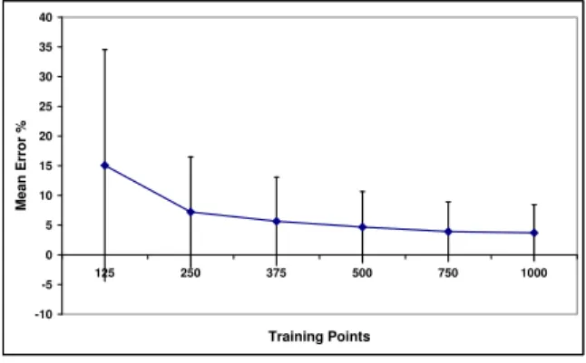
First we train a predictor per benchmark on randomly chosen configurations and predict energy-delay and execu-tion time for the same benchmark on new configuraexecu-tions. The results for varying number of training points are shown in Figure 7. As would be expected, increasing the size of the training set improves prediction accuracy significantly. For energy-delay, mean error across all the benchmarks for 125 training samples is 15.2%, dropping to 3.7% for 1000 training samples. For execution time, the mean error is 5.6% for 125 training samples and 0.9% for 1000. We see the error dropping as we increase the training set up to 1000 points.We expect small further improvements with
0 100 200 300 400 500 600 700 800 900 1000 0 0.5 1 1.5 2
Configurations sorted by energy delay
Normalized energy delay
Figure 5. Normalized energy-delay averaged across all benchmarks. Configurations are sorted by increasing energy-delay.
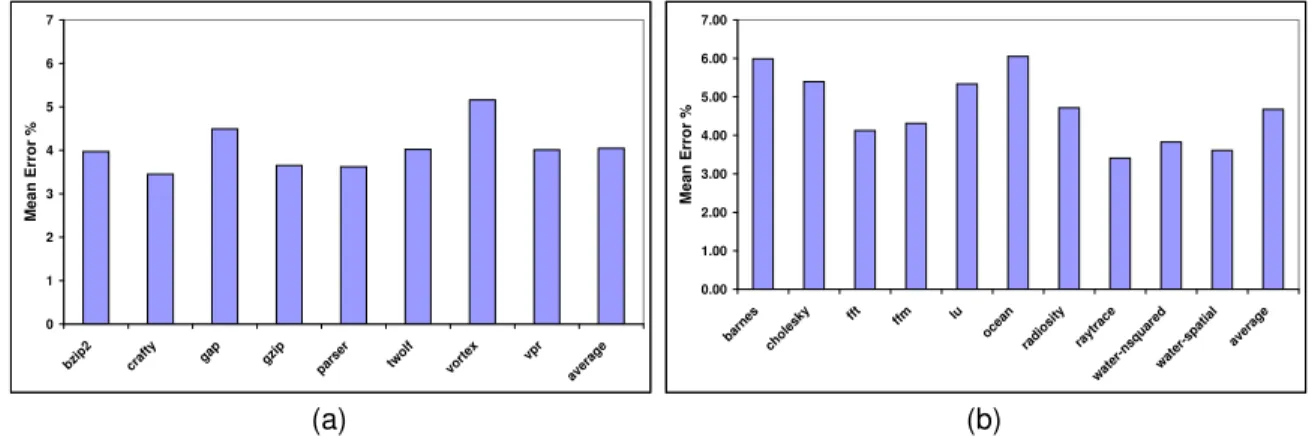
additional training points. Figures 8(a) and 8(b) show the mean error in energy-delay and performance prediction for the benchmarks when trained on 1000 configurations. We see that performance is more easily predicted with mean er-ror of 0.9% compared to energy-delay with 3.7% across the benchmarks. It can be seen from Figure 8 that there is some variation in the predictability of different programs. It is also interesting to see that, for the same number of train-ing samples, energy-delay is consistently harder to predict accurately. The three programs with worst prediction accu-racy are the same for energy-delay and performance:ocean,
choleskyandbarnes.
5.3
Cross-Program Prediction with Seen
Configurations
We now train a predictor using training points from N-1 benchmarks and attempt to do cross-program prediction. First we predict only configurations already seen in the
training set. We perform two sets of experiments. First
we train only on programs from the same benchmark suite as the program to be predicted. For all these predictions we use eight randomly chosen reactions. From Figure 9 we see that the predictor generalizes well across programs. We then predict each program with a model trained from all the other programs, from both suites. For all these predictions we again use eight randomly chosen reactions. The result-ing mean errors are in Figure 10. We see that the mean absolute error ranges between 3.4% forraytraceandcrafty
and 6.0% forocean, with a mean error of 3.9% across the benchmarks.
945 950 955 960 965 970 975 980 985 990 995 1.4 1.5 1.6 1.7 1.8 1.9 2 2.1 2.2 2.3 2.4
Configurations sorted by average energy delay
Normalized energy delay
bzip vpr fmm fft
Figure 6. Normalized energy-delay for four benchmarks. Configurations are sorted by increasing energy-delay.
5.4
Cross-Program Prediction for New
Configurations
Again, our training set consists of randomly sam-pled configurations from N-1 benchmarks, and we predict energy-delay and execution time forunseen configurations
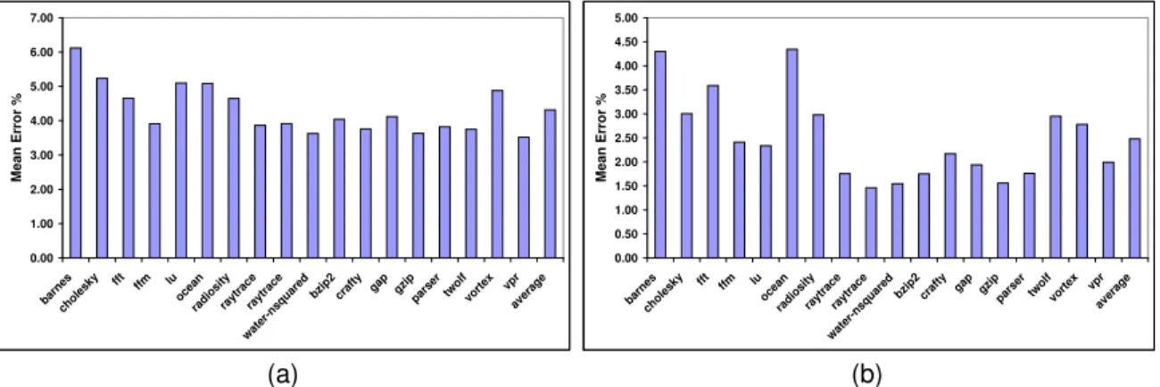
for the Nth benchmark. We first train models on each of the benchmark suites seperately. For each benchmark, we train the model on the rest of the programs from that bench-mark suite and repeat the process for each program. The mean prediction errors for 1000 training points per bench-mark are in Figure 11. We then put all the programs into one bag and cross predict performance and energy-delay. The results for this are detailed in Table 2. We evaluate predictions with different numbers of reactions, starting at zero. When no reactions are used for cross-program predic-tion, only the configuration vector is used for training and prediction. This incorporates no program specific informa-tion. This, surprisingly, performs relatively well. With 1000 training points per benchmark, mean error for energy-delay is 5.5% and that for performance is 4.2%. This suggests that the programs in the pool scale fairly similarly to each other across the configuration space. We can improve the prediction using reactions, however. When we extend the feature vector to use two reactions instead of none, we see the error rate drop by about 20% on average. We see fur-ther incremental improvements if we increase the number of reactions. We see that on some of the hard to predict bench-marks, the error rate drops sharply as we add reactions; by as much as 42% forwater-spatial. We also see the variance of the errors dropping with adding reactions. The change in the error as we change the number of reactions can be seen
graphically in Figure 13. For training with 1000 training points per benchmark, and using 8 reactions, the mean error observed in energy-delay predictions is 4.3%, and for 4 re-actions it is 4.5%. In contrast, if we train on samples from the same benchmark, we would require at least 500 to 750 samples to achieve the same prediction accuracy as we do with 4 or 8 reactions. Predictions for execution time show the same trend. The mean error for 8 reactions is 2.5% and for 4 reactions is 2.5% as well. This is better than the error obtained by training a model with 250 simulation results for just the same benchmark. Hence, using information from previously executed benchmarks, we can very quickly pre-dict the behaviour of a new program.
Error rates using cross-program prediction compare fa-vorably with the error rates observed when models are trained on the same program with many more simulations required. A direct comparison is made in Figure 2. As can be seen from the figure, this technique provides the option of trading less than 1% in mean absolute error for very sig-nificantly reducing the number of simulations needed.
-10 -5 0 5 10 15 20 25 30 35 40 125 250 375 500 750 1000 Training Points M e a n E rr o r %
Figure 7. Mean absolute error in energy-delay predictions for increasing size of training data.
6 RELATED WORK
6.1
Predictive Modeling for Architecture
Design Space Exploration
There has been significant interest recently in using pre-dictive modeling to accelerate design space exploration. We discuss the work most closely related to ours.
Recently, Ipeket al.[7] proposed the use of an ANN (Ar-tificial Neural Network) to predict the impact of hardware parameter variations (e.g., cache size, memory latency, etc) on the performance behavior of a target architecture. Af-ter training on less than 1% of the design space, the model
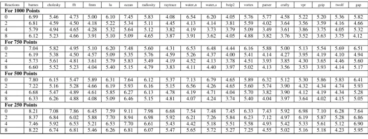
Reactions barnes cholesky fft fmm lu ocean radiosity raytrace water n water s bzip2 vortex parser crafty vpr gzip twolf gap For 1000 Points 0 6.99 5.46 4.73 5.00 6.10 7.45 5.83 4.08 6.54 6.20 4.05 5.76 5.77 4.58 5.22 5.20 5.36 5.82 2 6.81 4.59 4.50 4.18 5.22 5.34 5.11 4.45 4.13 4.14 3.81 5.59 4.02 3.64 3.56 3.59 4.16 4.66 4 5.79 4.94 4.65 4.28 5.32 5.64 5.12 3.82 4.19 3.73 3.79 5.09 3.49 3.61 3.86 3.75 4.05 5.32 8 6.12 5.23 4.66 3.91 5.10 5.09 4.65 3.87 3.91 3.62 4.05 4.88 3.82 3.76 3.52 3.63 3.75 4.12 For 750 Points 0 7.04 5.82 4.95 5.10 6.20 7.48 5.60 4.31 6.53 6.48 4.44 6.16 5.88 5.00 5.13 5.54 5.69 6.51 2 6.19 5.38 4.50 4.57 5.09 5.35 5.76 4.59 5.26 4.37 4.00 5.41 4.14 4.27 3.95 4.19 4.10 4.94 4 5.73 5.61 4.81 3.61 5.79 5.83 5.49 4.19 4.52 4.13 3.78 4.51 3.93 3.85 4.30 3.65 4.46 5.60 8 6.60 5.52 5.23 4.04 5.40 5.15 4.79 3.83 4.11 4.40 3.97 5.02 4.13 3.56 3.53 3.93 4.14 5.17 For 500 Points 0 7.80 6.15 5.47 5.89 6.31 7.64 6.12 5.37 7.13 6.79 4.65 5.89 6.32 5.12 5.30 5.86 5.83 6.41 2 7.22 5.16 5.28 4.66 6.19 5.93 6.16 5.15 6.56 4.26 4.65 5.60 5.74 3.90 4.32 4.34 4.74 5.93 4 6.68 5.47 4.89 4.61 5.85 6.27 6.13 4.78 4.19 4.71 4.04 5.70 3.82 3.90 4.12 4.19 4.34 5.28 8 6.33 6.26 4.88 4.08 5.09 6.46 5.15 4.81 4.07 4.24 3.74 5.40 4.04 3.97 3.64 4.02 4.15 5.05 For 250 Points 0 8.21 7.08 7.86 6.45 7.59 9.11 7.98 6.68 7.54 7.48 7.45 6.33 7.43 5.92 6.98 7.10 6.28 7.64 2 8.37 6.84 6.02 5.88 7.70 8.94 6.98 5.92 6.21 7.26 5.84 6.23 7.12 4.97 6.19 5.87 5.28 6.86 4 7.46 5.92 6.53 5.21 6.53 7.70 6.61 5.43 4.42 5.18 5.51 5.58 4.93 5.42 5.33 5.61 5.12 6.90 8 8.22 6.74 6.81 5.46 6.26 6.81 6.07 5.47 5.65 5.72 5.27 7.25 4.55 5.02 5.16 5.18 4.23 5.95
Table 2. Mean absolute error with varying number of reactions and training points for Splash-2 benchmarks 0.00 1.00 2.00 3.00 4.00 5.00 6.00 barne s chol esky fft ffm luocean radi osity rayt race wat er-ns qua red wat er-s patia l bzip2craf ty gapgzip pars er twol f vor tex vpr aver age % M e a n E rr o r (a) 0.00 0.50 1.00 1.50 2.00 2.50 barne s chol esky fft ffm luocean radi osity rayt race wat er-ns qua red wat er-s patia l bzip2craf ty gap gzip pars er twol f vor tex vpr aver age M e a n E rr o r % (b)
Figure 8. Mean absolute error of predictions for (a) energy-delay and (b) execution time. A model is trained per program from 1000 randomly sampled configurations for the same program.
can still accurately predict performance variations with less than 5% error. One model is built for each benchmark, i.e., the model does not learnacrossbenchmarks as ours does.
Lee and Brooks [11] use piecewise polynomial regres-sion to predict IPC and power on a multiprocessor design space. They obtain 4,000 random samples from a design space with approximately 1 billion points. Each sample maps a set of architectural and application-specific pre-dictors to observed performance and power. These sam-ples are used to formulate models that predict the perfor-mance and power of previously unseen architecture config-urations. The authors obtain error rates as low as 4.1% for performance and 4.3% for power. Again, the models are benchmark-specific, that is, several thousand sample points from the design space are required to build accurate models for any new program.
In another paper, Leeet al.[12] build predictors for mul-tiprocessor application performance when varying the ap-plication’s input parameters. They compare piecewise poly-nomial regression and neural network approaches on two multiprocessor applications for three different multiproces-sor platforms. Both regression and neural networks are accurate with median rates ranging from 2.2% to 10.5%. These models, too, need to be built per benchmark and no cross-program prediction is done.
Josephet al.[8] describe using radial basis functionRBF
networks to predict CPI for several SPEC CPU2000 bench-marks. The RBF’s can capture non-linear effects in the space being modeled and are compared to and outperform linear regression models. The models are benchmark, in-put, and architecture specific and a new model must be con-structed if either one of these changes. In contrast, the
mod-0 1 2 3 4 5 6 7 bzip2 craf ty gap gzip pars er twol f vor tex vpr aver age M e a n E rr o r % (a) 0.00 1.00 2.00 3.00 4.00 5.00 6.00 7.00 barne s chol esky fft ffm lu ocea n radi osity rayt race wat er-ns qua red wat er-s patia l aver age M e a n E rr o r % (b)
Figure 9. Mean absolute error for energy-delay predictions for (a) TLS programs and (b) Splash-2 programs. For each program predicted, the model is trained on 1000 configurations from each of the other programs in the same suite. Only configurations present in the training set are predicted.
0 1 2 3 4 5 6 7 8 bzip 2 craf ty gap gzip pars er two lf vort ex vpr aver age M ean E rr o r % (a) 0 1 2 3 4 5 6 7 8 barne s chol esky fft ffm lu ocean radi osity rayt race wat er-ns qua red wat er-s patia l aver age M e a n E rr o r % (b)
Figure 11. Mean absolute error for energy-delay predictions using 8 reactions for (a) TLS programs and (b) Splash-2 programs. For every prediction, the model is trained on 1000 configurations from each of the remaining programs of the same suite. Predictions are made for configurations not found in the training set.
els described in this paper can accurately predict new un-seen programs.
6.2
Fast Simulation Techniques
Orthogonal to the aforementioned techniques, and to ours, is the effort to cut down the time of individual simu-lations. Initial efforts to provide faster simulations resorted to simple truncated execution, that is, skipping a number of instructions to avoid capturing initialization behavior, and then simulating a further, hopefully representative, section of the program. Unfortunately, as noted in [24], the results obtained this way are in many cases far from representative. To alleviate this problem, statistical simulation tech-niques have been proposed. Sherwoodet al.[19] propose
first to profile the benchmark to find simulation points rep-resentative of the overall behavior and then simulating only those. The results obtained, are then further processed to generate the final simulation results. Ipek et. al. [7] demonstrate that this technique is mostly orthogonal to the use of ANN based predictive modeling. A similar approach has been followed by Wunderlichet al.[25], with the main difference being that profiling is not used to determine sim-ulation points. Instead, the simulated points are periodically selected. In order to avoid picking a sub-optimal sampling frequency, the mechanism tries to estimate the error and reg-ulate the frequency accordingly.
Karkhaniset al. [10] propose an analytical model for hardware exploration that captures the key performance fea-tures of superscalar processors. This model can potentially
0.00 1.00 2.00 3.00 4.00 5.00 6.00 7.00 barne s chol esky fft ffm lu ocea n radi osity rayt race rayt race wat er-ns qua red bzip2craf ty gapgzip pars er twol f vor tex vpr aver age M e a n E rr o r % (a) 0.00 0.50 1.00 1.50 2.00 2.50 3.00 3.50 4.00 4.50 5.00 barne s chol esky fft ffm lu ocea n radi osity rayt race rayt race wat er-ns qua red bzip2craf ty gap gzip pars er twol f vor tex vpr aver age M e a n E rr o r % (b)
Figure 12. Mean absolute error using 8 reactions for predictions of (a) energy-delay and (b) execution time. For every prediction, the model is trained on 1000 configurations each fromallof the remaining programs. Predictions are made for configurations not found in the training set.
0.00 1.00 2.00 3.00 4.00 5.00 6.00 7.00 barne s chol esky fft ffm lu ocea n radi osity rayt race wat er-ns qua red wat er-s patia l bzip2craf ty gap gzip pars er twol f vor tex vpr aver age M e a n E rr o r %
Figure 10. Mean absolute error for energy-delay prediction of all programs using 8 reac-tions. For each program predicted, the model is trained on 1000 configurations each from
all the other programs. Only configurations already present in the training set are pre-dicted.
be used for software exploration, unfortunately this work is not directly applicable to the multicore environment we are interested in. More specifically the model does not capture thread interaction due to shared resources which inevitably renders it inaccurate. Eeckhoutet al.[6] use statistical sim-ulation to similarly capture processor characteristics, and generate synthetic traces that are later run on a simplified superscalar simulator. After any program transformation, a new trace needs to be generated if this approach were to be used for software exploration, requiring a full functional simulation.
Recently, IBM has highlighted the issue of software
tun-0 1 2 3 4 5 6 7 8 250 500 750 1000 Training Points % M e a n E rror
0 Reactions 2 Reactions 4 Reactions 8 Reactions
Figure 13. Average Mean Error with varying number of reactions and training points.
ing early on in the design cycle. For the Blue Gene/L, it was shown that an approximate but fast performance model, as a replacement for more detailed but slow simulators, can be very useful in practice [2]; still, the approximate model proposed was designed manually and in an ad-hoc manner.
6.3
Predictive Modeling for Compilation
Machine learning has recently also been investigated by a number of researchers in the area of compiler optimiza-tion. Much of the prior work in machine learning-based compilation relies onprogram feature-based characteriza-tion. For instance, Monsifrot et al. [16], Stephenson et al.[22], and Agakovet al.[1] all use static loop nest fea-tures. Cavazoset al.[5] considered a reaction-based scheme that uses the sequence of transformations applied to a pro-gram as an input to a learnt model.
7
CONCLUSIONS
In this paper we evaluate cross-program prediction to speed up the exploration of CMP design spaces. We employ neural network based predictive models to predict energy-delay and execution time. For cross-program prediction, we use a technique based on reactions to allow prediction for new programs with a very small number of additional sim-ulations, once the model has been built for other programs. We show that for two parallel application classes, Thread Level Speculation (TLS) and the Splash-2 benchmarks, we can get prediction accuracies similar to a model learnt with many hundreds of configuration points (involving running as many simulations) with as little as 2-8 reactions, thus re-sulting in a significant reduction in simulation time for these predictions.
REFERENCES
[1] F. Agakov, E. Bonilla, J.Cavazos, B.Franke, G. Fursin, M. O’Boyle, J. Thomson, M. Toussaint, and C. Williams. “Using Machine Learn-ing to Focus Iterative Optimization.” Intl. Symp. on Code Genera-tion and OptimizaGenera-tion, pages 295-308, March 2006.
[2] L. Bachega, J. Brunheroto, L. DeRose, P. Mindlin, and J. Moreira. “The Bluegene/L Pseudo Cycle-Accurate Simulator.”Intl. Symp. on Performance Analysis of Systems and Software, pages 36-44, March 2004.
[3] H. Berry, D. G. Prez, and O. Temam. “Chaos in computer perfor-mance.”Chaos, 16(1), December 2005.
[4] C. Bishop.Neural Networks for Pattern Recognition. Oxford Uni-versity Press, 2005.
[5] J. Cavazos, C. Dubach, F. Agakov, E. Bonilla, M. O’Boyle, G. Fursin, and O. Temam. “Automatic Performance Model Con-struction for the Fast Software Exploration of New Dardware De-signs.” Intl. Workshop on Compiler and Architecture Support for Embedded Systems, pages 24-34, October 2006.
[6] L. Eeckhout, R. H. Bell Jr., B. Stougie, K. D. Bosschere, and L. K. John. “Control Flow Modeling in Statistical Simulation for Accu-rate and Efficient Processor Design Studies.” Intl. Symp. on Com-puter Architecture, pages 350–363, June 2004.
[7] E. Ipek, S. A. McKee, B. R. de Supinski, M. Schulz, and R. Caru-ana. “Efficiently Exploring Architectural Design Spaces via Predic-tive Modeling.”Intl. Conf. on Architectural Support for Program-ming Languages and Operating Systems, pages 195-206, October 2006.
[8] P. J. Joseph, K. Vaswani and M. J. Thazhuthaveetil. “A Predictive Model for Superscalar Processor Performance.” Intl. Symp. on Mi-croarchitecture, pages 161-70, December 2006.
[9] S. Jourdan, J. Stark, T. H. Hsing, and Y. N. Patt. “Recovery Require-ments of Branch Prediction Storage Structures in the Presence of Mispredicted-Path Execution.”Intl. Journal of Parallel Program-ming, 25(5), pages 363-383, 1997.
[10] T. Karkhanis and J. E. Smith. “A First-Order Superscalar Processor Model.”Intl. Symp. on Computer Architecture, pages 338–349, June 2004.
[11] B. C. Lee and D. M. Brooks. “Accurate and Efficient Regression Modeling for Microarchitectural Performance and Power Predic-tion.”Intl. Conf. on Architectural Support for Programming Lan-guages and Operating Systems, pages 185-194, October 2006. [12] B. C. Lee, D. M. Brooks, B. R. de Supinski, M. Schulz, K. Singh,
and S. A. McKee. “Methods of Inference and Learning for Perfor-mance Modeling of Parallel Applications.”Symp. on Principles and Practice of Parallel Programming, pages 249-258, March 2007. [13] W. Liu, J. Tuck, L. Ceze, W. Ahn, K. Strauss, J. Renau, and J.
Tor-rellas. “POSH: A TLS Compiler that Exploits Program Structure.”
Symp. on Principles and Practice of Parallel Programming, pages 158-167, March 2006.
[14] D. J. C. MacKay. “Bayesian Interpolation.” Neural Computation, 4(3), pages 415-447, 1992.
[15] S. McFarling. “Combining Branch Predictors.” WRL Technical
Note, TN-36, 1993.
[16] A. Monsifrot, F. Bodin, and R. Quiniou. “A Machine Learning Approach to Automatic Production of Compiler Heuristics.” Intl. Conf. on Artificial Intelligence: Methodology, Systems, Applica-tions, LNCS 2443, pages 41–50, 2002.
[17] J. Renau, B. Fraguela, J. Tuck, W. Liu, M. Prvulovic, L. Ceze, S. Sarangi, P. Sack, K. Strauss, and P. Montesinos. SESC Simulator.
http://sesc.sourceforge.net, January 2005.
[18] J. Renau, J. Tuck, W. Liu, L. Ceze, K. Strauss, and J. Torrellas. “Tasking with Out-of-Order Spawn in TLS Chip Multiprocessors: Microarchitecture and Compilation.” Intl. Conf. on Supercomput-ing, pages 179-188, June 2005.
[19] T. Sherwood, E. Perelman, G. Hamerly, and B. Calder. “Automati-cally Characterizing Large Scale Program Behavior.”Intl. Symp. on Architectural Support for Programming Languages and Operating Systems, pages 45-57, December 2002.
[20] P. Shivakumar, and N. P. Jouppi. CACTI 3.0: An Integrated Cache Timing, Power, and Area Model.WRL Research Report, 2001/2. [21] SPEC Benchmark Suite.http://www.spec.org.
[22] M. Stephenson and S. P. Amarasinghe. “Predicting Unroll Factors Using Supervised Classification.” Intl. Symp. on Code Generation and Optimization, pages 123-134, March 2005.
[23] S. C. Woo, M. Ohara, E. Torrie, J. P. Singh, and A. Gupta. “The SPLASH-2 Programs: Characterization and Methodological Con-siderations.”Intl. Symp. on Computer Architecture, pages 24-36, June 1995.
[24] J. J. Yi, S. V. Kodakara, R. Sendag, D. J. Lilja, and D. M. Hawkins. “Characterizing and Comparing Prevailing Simulation Techniques.”
Intl. Symp. on High-Performance Computer Architecture, pages 266-277, February 2005.
[25] R. Wunderlich, T. F. Wenish, B. Falsafi, and J. C. Hoe. “SMARTS: Accelerating Microarchitectural Simulation via Rigorous Statistical Sampling”Intl. Symp. on Computer Architecture, pages 84-95, June 2003.