NBER WORKING PAPER SERIES
THE CENTRAL-BANK BALANCE SHEET AS AN INSTRUMENT OF MONETARY POLICY
Vasco Curdia Michael Woodford Working Paper 16208
http://www.nber.org/papers/w16208
NATIONAL BUREAU OF ECONOMIC RESEARCH 1050 Massachusetts Avenue
Cambridge, MA 02138 July 2010
Prepared for the 75th Carnegie-Rochester Conference on Public Policy, "The Future of Central Banking,'' April 16-17, 2010. We thank Harris Dellas, Gauti Eggertsson, Marvin Goodfriend, Bob Hall, James McAndrews, Shigenori Shiratsuka, Oreste Tristani, Kazuo Ueda and Tsutomu Watanabe for helpful discussions, Ging Cee Ng for research assistance, and the NSF for research support of the second author. The views expressed in this paper are those of the authors and do not necessarily reflect positions of the Federal Reserve Bank of New York, the Federal Reserve System, or the National Bureau of Economic Research.
NBER working papers are circulated for discussion and comment purposes. They have not been peer-reviewed or been subject to the review by the NBER Board of Directors that accompanies official NBER publications.
© 2010 by Vasco Curdia and Michael Woodford. All rights reserved. Short sections of text, not to exceed two paragraphs, may be quoted without explicit permission provided that full credit, including © notice, is given to the source.
The Central-Bank Balance Sheet as an Instrument of Monetary Policy Vasco Curdia and Michael Woodford
NBER Working Paper No. 16208 July 2010
JEL No. E52,E58
ABSTRACT
While many analyses of monetary policy consider only a target for a short-term nominal interest rate, other dimensions of policy have recently been of greater importance: changes in the supply of bank reserves, changes in the assets acquired by central banks, and changes in the interest rate paid on reserves. We extend a standard New Keynesian model to allow a role for the central bank's balance sheet in equilibrium determination, and consider the connections between these alternative dimensions of policy and traditional interest-rate policy. We distinguish between “quantitative easing” in the strict sense and targeted asset purchases by a central bank, and argue that while the former is likely be ineffective at all times, the latter dimension of policy can be effective when financial markets are sufficiently disrupted. Neither is a perfect substitute for conventional interest-rate policy, but purchases of illiquid assets are particularly likely to improve welfare when the zero lower bound on the policy rate is reached. We also consider optimal policy with regard to the payment of interest on reserves; in our model, this requires that the interest rate on reserves be kept near the target for the policy rate at all times.
Vasco Curdia
Federal Reserve Bank of New York 33 Liberty Street, 3rd Floor
New York, NY 10045 Vasco.Curdia@ny.frb.org Michael Woodford Department of Economics Columbia University 420 W. 118th Street New York, NY 10027 and NBER michael.woodford@columbia.edu
An online appendix is available at:
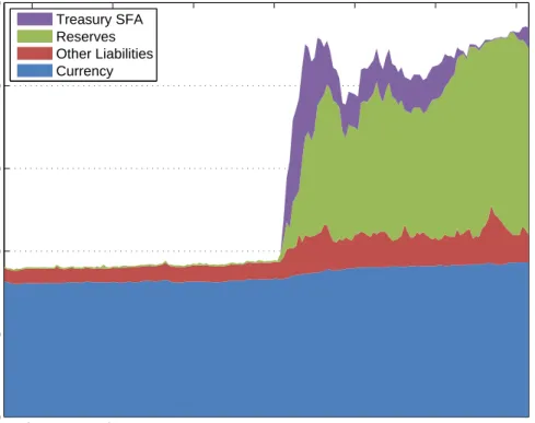
The recent global financial crisis has confronted central banks with a number of questions beyond the scope of standard accounts of the theory of monetary policy. Monetary policy is ordinarily considered solely in terms of the choice of an operating target for a short-term nominal interest rate, such as the federal funds rate in the case of the Federal Reserve. Yet during the recent crisis, other dimensions of policy have occupied much of the attention of central bankers. One is the question of the appropriate size of the central bank’s balance sheet. In fact, the Fed’s balance sheet has grown dramatically in size since the fall of 2008 (Figures 1 and 2).
As shown in Figure 1, the component of the Fed’s liabilities constituted by reserves held by depository institutions has changed in an especially remarkable way: by the fall of 2008 reserves were more than 100 times larger than they had been only a few months earlier. This explosive growth has led some commentators to suggest that the main instrument of US monetary policy has changed, from an interest-rate policy to one often described as “quantitative easing.” Does it make sense to regard the supply of bank reserves (or perhaps the monetary base) as an alternative or superior operating target for monetary policy? Does this (as some would argue) become the only important monetary policy decision once the overnight rate (the federal funds rate) has reached the zero lower bound, as it effectively has in the US since December 2008? And now that the Federal Reserve has legal authorization to pay interest on reserves (under the Emergency Economic Stabilization Act of 2008), how should this additional potential dimension of policy be used?
The past two years have also seen dramatic developments with regard to the composition of the asset side of the Fed’s balance sheet (Figure 2). Whereas the Fed had largely held Treasury securities on its balance sheet prior to the fall of 2007, other kinds of assets — a variety of new “liquidity facilities”, new programs under which the Fed essentially became a direct lender to certain sectors of the economy, and finally targeted purchases of certain kinds of assets, including more than a trillion dollars’ worth of mortgage-backed securities — have rapidly grown in importance, and decisions about the management of these programs have occupied much of the attention of policymakers during the recent period. How should one think about the aims of these programs, and the relation of this new component of Fed policy to traditional interest-rate policy? Is Federal Reserve credit policy a substitute
for interest-rate policy, or should it be directed to different goals than those toward which interest-rate policy is directed?
These are clearly questions that a theory of monetary policy adequate to our present cir-cumstances must address. Yet not only have they been the focus of relatively little attention until recently, but the very models commonly used to evaluate the effects of alternative pre-scriptions for monetary policy have little to say about them. Many models used for monetary policy analysis — both theoretical models used in normative discussions of ideal monetary policy commitments, and quantitative models used for numerical simulation of alternative policies — abstract altogether from the central bank’s balance sheet, simply treating a short-term nominal interest rate as if it were under the direct control of the monetary authorities, and analyzing how that interest rate should be adjusted.1 But such a framework rules out
the kinds of questions that have recently preoccupied central bankers from the start.
In this paper, we extend a basic New Keynesian model of the monetary transmission mechanism to explicitly include the central bank’s balance sheet as part of the model. In addition to making more explicit the ways in which a central bank is able to (indirectly) exert control over the policy rate, the extended model allows us to address questions about other dimensions of policy of the sort just posed. In order to make these questions non-trivial, we also introduce non-trivial heterogeneity in spending opportunities, rather than adopting the familiar device of the “representative household,” so that financial intermediation matters for the allocation of resources; we introduce imperfections in private financial intermediation, and the possibility of disruptions to the efficiency of intermediation, for reasons taken here as exogenous, so that we can examine how such disturbances affect the desirability of central-bank credit policy; and we allow central-central-bank liabilities to supply transactions services, so that they are not assumed to be perfect substitutes for privately-issued financial instruments of similar maturity and with similar state-contingent payoffs. Finally, we consider the con-duct of policy both when the zero lower bound on the policy rate is not a binding constraint, and also when it is.
In section 1, we begin with a general discussion of whether (and when) one should expect aspects of the central bank’s balance sheet to matter for equilibrium determination. This
is intended both to motivate our modeling exercise, by explaining what features a model must have in order for policies affecting the balance sheet to be of possible significance, and to introduce some important distinctions among alternative dimensions of policy. Section 2 outlines the structure of our model, with primary attention to the way that we model financial intermediation and the policy choices available to the central bank. Section 3 then uses the model to discuss changes in the supply of bank reserves as a dimension of policy, and the related question of the rate of interest that should be paid on reserves. Section 4 turns to the question of the optimal composition of the central bank’s asset portfolio, considering the conditions under which the traditional “Treasuries only” policy would be optimal in the context of our model. Section 5 then considers the optimal size and duration of central-bank credit policy in those cases where “Treasuries only” is not the optimal policy, and section 6 concludes.
1
When
Does
the
Central-Bank
Balance
Sheet
Matter?
It might be thought that monetary policy analysis would haveto be involve explicit consid-eration of the central bank’s balance sheet, at least to the extent that one believes in the importance of general-equilibrium analysis. Yet monetary DSGE models often abstract from any discussion of the central bank’s balance sheet. In fact, this is not only possible (in the sense that the models have at least a logically consistent structure), but is quite innocuous, under a certain idealized view of the functioning of financial markets. Neither the size nor the composition of the central bank’s balance sheet matter for equilibrium prices or quan-tities except because of financial imperfections. This is important, both to understand why additional dimensions of policy may suddenly become relevant when the smooth functioning of financial markets can no longer be taken for granted, and to understand why we emphasize certain types of frictions in our analysis below. The introduction of credit frictions requires a significant complication of our analysis, and before undertaking this modeling effort, it may be useful to clarify why our assumptions about credit frictions are essential to the conclusions
that we obtain.
1.1
An Irrelevance Result
It is often supposed that open-market purchases of securities by the central bank must inevitably affect the market prices of those securities (and hence other prices and quantities as well), through what is called a “portfolio-balance effect”: if the central bank holds less of certain assets and more of others, then the private sector is forced (as a requirement for equilibrium) to hold more of the former and less of the latter, and a change in the relative prices of the assets will almost always be required to induce the private parties to change the portfolios that they prefer. In order for such an effect to exist, it is thought to suffice that private parties not be perfectly indifferent between the two types of assets; and there are all sorts of reasons why differences in the risky payoffs associated with different assets should make them not perfect substitutes, even in a world with frictionless financial markets.2
But this doctrine is inconsistent with the general-equilibrium theory of asset prices, at least to the extent that financial markets are modeled as frictionless. It is clearly inconsistent with a representative-household asset pricing theory (even though the argument sketched above makes no obvious reference to any heterogeneity on the part of private investors). In the representative-household theory, the market price of any asset should be determined by the present value of the random returns to which it is a claim, where the present value is calculated using an asset pricing kernel (stochastic discount factor) derived from the repre-sentative household’s marginal utility of income in different future states of the world. Insofar as a mere re-shuffling of assets between the central bank and the private sector should not change the real quantity of resources available for consumption in each state of the world, the representative household’s marginal utility of income in different states of the world should not change. Hence the pricing kernel should not change, and the market price of one unit of a given asset should not change, either, assuming that the risky returns to which the asset represents a claim have not changed.
The flaw in the “portfolio-balance” theory is the following. It assumes that if the private 2Explanations by central banks of what they believe is accomplished by targeted asset purchases frequently
sector is forced to hold a portfolio that includes more exposure to a particular risk — say, a low return in the event of a real-estate crash — then private investors’ willingness to hold that particular risk will be reduced: investors will anticipate a higher marginal utility of income in the state in which the real-estate crash occurs, and so will pay less than before for securities that have especially low returns in that state. But the fact that the central bank takes the real-estate risk onto its own balance sheet, and allows the representative household to hold only securities that pay as much in the event of a crash as in other states, does not make the risk disappear from the economy. The central bank’s earnings on its portfolio will be lower in the crash state as a result of the asset exchange, and this will mean lower earnings distributed to the Treasury, which will in turn mean that higher taxes will have to be collected by the government from the private sector in that state; so the representative household’s after-tax income will be just as dependent on the real-estate risk as before. This is why the asset pricing kernel does not change, and why asset prices are unaffected by the open-market operation.3
The irrelevance result is easiest to derive in the context of a representative-household model, but in fact it does not depend on the existence of a representative household, nor upon the existence of a complete set of financial markets. All that one needs for the argument are the assumptions that (i) the assets in questionare valued only for their pecuniary returns
— they may not be perfect substitutes from the standpoint of investors, owing to different risk characteristics, but not for any other reason — and that (ii) all investors can purchase arbitrary quantities of the same assets at the same (market) prices. Under these assumptions, the irrelevance of central-bank open-market operations is essentially a Modigliani-Miller result, as noted by Wallace (1981). If the central bank buys more of assetxby selling shares of asset y, private investors should wish purchase more of asset y and divest themselves of asset x, by exactly the amounts that undo the effects of the central bank’s trades. The reason that they optimally choose to do this is in order to hedge the additional tax/transfer income risk that they take on as a result of the change in the central bank’s portfolio. If share θh of the returns on the central bank’s portfolio are distributed to household h, where
3Eggertsson and Woodford (2003) show in the context of a representative-household model that it does
the {θh} are a set of weights that sum to 1, then household h should choose a trade that
cancels exactly fraction θh of the central bank’s trade, in order to afford exactly the same
state-contingent consumption stream as before. Summing over all households, the private sector chooses trades that in aggregate precisely cancel the central bank’s trade. The result obtains even if different households have very different attitudes toward risk, different time profiles of income, different types of non-tradeable income risk that they need to hedge, and so on, and regardless of how large or small the set of marketed securities may be. One can easily introduce heterogeneity of the kind that is often invoked as an explanation of time-varying risk premia without this implying that any “portfolio-balance” effects of central-bank transactions should exist.
As Wallace (1981) notes, this implies thatboththe size and the composition of the central-bank balance sheet should be irrelevant for market equilibrium in a world with frictionless financial markets (more precisely, a world in which the two postulates hold). This does not,
however, mean, as is sometimes thought, thatmonetary policyis irrelevant in such a world; it simply means that monetary policy cannot be implemented through open-market operations. Control of a short-term nominal interest rate by the central bank remains possible in the frictionless environment. The central bank is still free to determine the nominal interest rate on overnight balances at the central bank as an additional dimension of policy (alongside its decisions about the quantity of liabilities to issue and the particular types of assets that it buys with them).4 This interest rate must then be linked in equilibrium to other short-term
interest rates, through arbitrage relations; and hence the central bank can determine the level of short-term nominal interest rates in general. Moreover, the central bank’s adjustment of nominal interest rates matters for the economy. Even in an endowment economy with flexible prices for all goods, the central bank’s interest-rate policy can determine the evolution of the general level of prices in the economy; in a production economy with sticky prices and/or wages, it can have important real effects as well.5
4The existence of these three independent dimensions of central-bank policy is discussed further below in
section 2.3, in the context of an explicit model.
5Both the way in which the central bank can determine the level of short-term interest rates in a frictionless
economy, and the macroeconomic implications of interest-rate policy in such models, are treated in detail in Woodford (2003, chaps. 2, 4).
In analyzing monetary policy options for a world of this kind, there would be no need to include the central bank’s balance sheet in one’s model at all: it would suffice that the short-term nominal interest rate be one of the asset prices in the model, and that it be treated as under the control of a monetary authority. This provides a potential justification for the use of “cashless” models in monetary policy analysis, in which no balance-sheet quantities at all appear.6 At the same time, the assumptions required for the irrelevance result are still
fairly strong (even if not so special as discussions of “portfolio-balance” effects often seem to assume), and it worth considering the consequences of relaxing them.
1.2
Allowing a Transactions Role for Central-Bank Liabilities
Many readers of Wallace (1981) are likely to have found the result paradoxical, and doubted the practical relevance of the entire line of reasoning, for one reason in particular. Wallace’s result implied, not only that exchanges of Treasuries for mortgage-backed securities by the Federal Reserve, holding fixed the overall size of the Fed’s balance sheet, should have no effect, but also that increases in the supply of bank reserves as a result of open-market purchases of Treasuries should have no effect. Yet the latter kind of operation had long been routinely used by the Fed to bring about desired changes in the federal funds rate, as every undergraduate learns. The theory seemed patently inapplicable to the operations of actual central banks in actual market economies.
Moreover, it is clear that overnight balances at the Fed have often been held despite being dominated in rate of return; until October 2008, these balances earned a zero nominal return, while other overnight interest rates (such as the federal funds rate) were invariably higher, for reasons that cannot be attributed purely to default risk. A natural (and thoroughly 6Of course, no one has proposed that any actual economies literally satisfy the two postulates; in
partic-ular, some central-bank liabilities are clearly valued in ways that are inconsistent with the two postulates. The use of “cashless” models for practical monetary policy analysis accordingly requires a further argument, which is that the transactions frictions that account for the observed demand for base money are not likely to make a large quantitative difference for the structural relations that matter for the analysis of alternative interest-rate policies, even if they matter a great deal for the precise way in which a central bank is able to implement interest-rate policy. See, e.g.,McCallum (2000, 2001), Woodford (2003, chap. 2, sec. 3, and chap. 4, sec. 3), and Ireland (2004).
conventional) inference is that this particular asset is (or at least, has often been) held for reasons beyond its pecuniary return alone; we may suppose that reserves at the Fed (and base money more generally) supply transactions services, by relaxing constraints that would otherwise restrict the transactions in which the holders of the asset can engage. The existence of these non-pecuniary returns — which may be modeled using any of a variety of familiar devices — will invalidate the Wallace (1981) neutrality result, at least insofar as open-market purchases of securities that increase the supply of reserves are concerned.
We can introduce a transactions role for reserves, or for liabilities of the central bank more generally, however, while still entertaining the hypothesis that with regard toall assets other than monetary liabilities of the central bank,the two postulates still hold: assets other than “money” are valued only for their pecuniary returns, and all investors can purchase arbitrary quantities of any of these assets at the same (market) prices. In this case, a weaker irrelevance result for central-bank trades still applies. No open-market operation that changes the composition of the central bank’s asset portfolio, while keeping unchanged the outstanding volume of the monetary liabilities of the central bank, should have any effects on asset prices, goods prices, or the allocation of resources.7 Again, the argument is essentially
a Modigliani-Miller theorem, and holds despite an arbitrary degree of heterogeneity in the situations of different households, and regardless of the size of the set of traded securities.
The result in this case validates the classic monetarist position: the supply of monetary liabilities by the central bank matters for macroeconomic equilibrium, but it does not matter at all what kinds of assets might “back” those liabilities on the other side of the central bank’s balance sheet, or how the base money gets to be in circulation. Hence a generation or two of texts in monetary economics have found it convenient to analyze monetary policy using models in which there is no central-bank balance sheet — merely a government printing press which creates additional “money” at a greater or lesser rate, which is then put in the hands of private parties, perhaps by dropping it from helicopters. Again, the omission is completely justifiable, if financial markets function efficiently enough for the two postulates to hold, except for the qualification regarding the special properties of “money.”
7This is the result obtained by Eggertsson and Woodford (2003), in the context of a
Under this view, there would be still be no ground for viewing targeted asset purchases as a relevant dimension of central-bank policy, though variations in the supply of monetary central-bank liabilities would matter. It might seem, then, Bernanke’s (2009) assertion that the Federal Reserve’s expansion of its balance sheet in the fall of 2008 represented “credit easing” rather than “quantitative easing” had matters backward: that the only real effect that should have been expected would have resulted from the expansion in the supply of bank reserves, regardless of the nature of the lending financed by that expansion in reserves. Yet this is not the conclusion that we draw at all. Expansion of the supply of bank reserves stimulates aggregate demand under normal circumstances, because it has ordinarily been the means by which the Fed has lowered the federal funds rate; yet once the supply of reserves is sufficient to drive the funds rate essentially to zero (as has been the case since late in 2008), there is no reason to expect further increases in the supply of reserves to increase aggregate demand any further, as we explain in the context of an explicit model in section 3. Once banks are no longer foregoing any otherwise available pecuniary return in order to hold reserves, there is no reason to believe that reserves continue to supply any liquidity services at the margin; and if they do not, the Modigliani-Miller reasoning applies once again to open market operations that increase the supply of reserves, just as in the model of Wallace.
While this reasoning cannot correctly be applied to conclude that open-market securities purchases that increase the supply of reserves canneverhave any effect, it can quite plausibly be used to conclude that such purchases should have no effect once the opportunity cost of reserves has fallen to zero. (It is fairly obvious that an open-market purchase of riskless short-term Treasury securities by issuing similarly riskless nominal short-term liabilities of the Fed should have no effect, once there is no longer any shortage of cash. But if pure changes in the central bank’s asset portfolio have no effect, then an increase in reserves to purchase short-term Treasuries should have the same effect as an increase in reserves to purchase some other asset, which effect must then be zero.) Hence it is not plausible that “quantitative easing” can be an effective strategy for providing further monetary stimulus once the zero lower bound is reached.
1.3
Do Targeted Asset Purchases Ever Matter?
The previous analysis suggests that Bernanke (2009) was right to be skeptical about the effectiveness of “quantitative easing.” But is there any more reason to expect “credit easing” to be of avail? Under the two postulates mentioned above, the answer is no. Yet there is some evidence suggesting that at least some of the Fed’s special credit facilities, and similar programs of other central banks, have affected asset prices8
As a simple example, Figure 3 shows the behavior of the spreads between yields on various categories of commercial paper and the one-month overnight interest-rate swap rate (essentially, a market forecast of the average federal funds rate over that horizon), over the period just before and after the introduction of the Fed’s Commercial Paper Funding Facility at the beginning of October 2008. (The darkest solid line shows the quantity of purchases of commercial paper by the Fed, which spikes up sharply at the introduction of the new facility.) The reason for the introduction of the new facility had been a significant disruption of the commercial paper market, indicated by the explosion of spreads in September 2008 for all four of the types of commercial paper shown in the figure. The figure also shows that spreads came back down again immediately with the introduction of the new facility, for three of the classes of paper (all except the A2/P2 paper) — these three series being precisely the ones for commercial paper of types that qualified for purchases under the CPFF. The spread for the A2/P2 paper instead remained high for several more months, though this spread as well has returned to more normal levels eventually, with the general improvement of financial conditions.9
Not only the sudden reduction in spreads for the other three types of paper, but the fact that spreads did not decline in the case of paper not eligible for purchase by the new facility, suggests that targeted asset purchases by the Fed did change the market prices of the assets in question. Hence some further modification of the two postulates is required in 8See,e.g.,Ashcraftet al. (2010), Babaet al. (2006), Gagnonet al. (2010), Sarkar (2009) and Sarkar and
Shrader (2010). For skeptical readings of the evidence, see instead Taylor (2009) and Stroebel and Taylor (2009).
9For further discussion of the crisis in the commercial paper market, this Fed program, and its effects,
order to allow a realistic analysis of the effects of programs of this kind. We propose that it is the assumption that all investors have equal opportunities to invest in all assets on the same terms that must be modified. If only certain specialists have the expertise required to invest in commercial paper, then developments that adversely affect the capital of those specialists (or their ability to fund themselves) can result in an increase in commercial paper yields relative to those on other instruments of similar maturity, as occurred in the fall of 2008. And central-bank purchases of commercial paper will not be offset by a corresponding reduction in private-sector purchases of that specific asset — even if the implications of the policy for state-contingent tax liabilities are correctly understood by everyone — if the parties whose state-contingent tax liabilities change are largely investors whocannotinvest in commercial paper in any event, and so cannot hold less of it even if the central bank’s action causes them to bear more income risk that is correlated with commercial-paper returns.
Hence in developing a model to assess the conditions under which “unconventional” dimensions of monetary policy may be relevant, it is important that we not assume that all financial-market participants can costlessly trade the same set of financial instruments. (A fortiori, it is important that we not adopt the simplification of assuming a representative agent.) In the next section, we sketch a relatively simple model that possesses the minimal elements required for a non-trivial discussion of the issues raised in the introduction.10
We assume heterogeneity in the spending opportunities available to different households at any point in time, so that some will have a motive to borrow while others are willing to save; and we assume that the households without current urgent needs for funds lack the expertise required to directly extend credit themselves to the borrowing households, so that they must instead deposit funds with competitive intermediaries who are in turn able to offer loan contracts to the borrowing households. We also allow the central bank a choice between holding “liquid” assets (Treasury debt) that can also be held by saving households on the same terms, and “illiquid” assets (the debt of private borrowers) that can otherwise only be held by the specialist intermediaries. Finally, we allow the central bank to create liabilities (reserves) that supply liquidity services, and so may be held in equilibrium even 10Other recent examples of DSGE models that can be used to address some of these same issues include
when they earn a lower interest rate than that on Treasury debt.
We model these various frictions in relatively reduced-form ways; our interest here is not in illuminating the sources of the frictions, but in exploring their general-equilibrium consequences. In particular, we wish to understand the extent to which they give rise to a multiplicity of independent dimensions for central-bank policy, and the interrelations that exist between variations of policy along these separate dimensions.
2
A Model with Multiple Dimensions of Monetary
Policy
Here we sketch the key elements of our model, which extends the model introduced in C´urdia and Woodford (2009a) to introduce the additional dimensions of policy associated with the central bank’s balance sheet. (The reader is referred to our earlier paper, and especially its technical appendix, for more details.)
2.1
Heterogeneity and the Allocative Consequences of Credit Spreads
Our model is a relatively simple generalization of the basic New Keynesian model used for the analysis of optimal monetary policy in sources such as Goodfriend and King (1997) and Woodford (2003). The model is still highly stylized in many respects; for example, we abstract from the distinction between the household and firm sectors of the economy, and instead treat all private expenditure as the expenditure of infinite-lived household-firms, and we similarly abstract from the consequences of investment spending for the evolution of the economy’s productive capacity, instead treating all private expenditure as if it were non-durable consumer expenditure (yielding immediate utility, at a diminishing marginal rate).
We depart from the assumption of a representative household in the standard model, by supposing that households differ in their preferences. Each household iseeks to maximize a
discounted intertemporal objective of the form E0 ∞ X t=0 βt · uτt(i)(c t(i);ξt)− Z 1 0 vτt(i)(h t(j;i) ;ξt)dj ¸ , (2.1)
where τt(i)∈ {b, s} indicates the household’s “type” in period t. Here ub(c;ξ) and us(c;ξ)
are two different period utility functions, each of which may also be shifted by the vector of aggregate taste shocksξt,andvb(h;ξ) andvs(h;ξ) are correspondingly two different functions
indicating the period disutility from working. As in the basic NK model, there is assumed to be a continuum of differentiated goods, each produced by a monopolistically competitive supplier;ct(i) is a Dixit-Stiglitz aggegator of the household’s purchases of these differentiated
goods. The household similarly supplies a continuum of different types of specialized labor, indexed by j, that are hired by firms in different sectors of the economy; the additively separable disutility of work vτ(h;ξ) is the same for each type of labor, though it depends on
the household’s type and the common taste shock.
Each agent’s type τt(i) evolves as an independent two-state Markov chain. Specifically,
we assume that each period, with probability 1−δ (for some 0 ≤ δ < 1) an event occurs which results in a new type for the household being drawn; otherwise it remains the same as in the previous period. When a new type is drawn, it is b with probabilityπb and s with
probabilityπs, where 0< πb, πs<1, πb+πs= 1.(Hence the population fractions of the two
types are constant at all times, and equal to πτ for each type τ .) We assume moreover that ub
c(c;ξ)> usc(c;ξ)
for all levels of expenditure c in the range that occur in equilibrium. Hence a change in a household’s type changes its relative impatience to consume, given the aggregate stateξt; in addition, the current impatience to consume of all households is changed by the aggregate disturbanceξt. We also assume that the marginal utility of additional expenditure diminishes at different rates for the two types, as is also illustrated in the figure; typebhouseholds (who are borrowers in equilibrium) have a marginal utility that varies less with the current level of expenditure, resulting in a greater degree of intertemporal substitution of their expenditures in response to interest-rate changes. Finally, the two types are also assumed to differ in the marginal disutility of working a given number of hours; this difference is calibrated so
that the two types choose to work the same number of hours in steady state, despite their differing marginal utilities of income. For simplicity, the elasticities of labor supply of the two types are not assumed to differ.
The coexistence of the two types with differing impatience to consume creates a social function for financial intermediation. In the present model, as in the basic New Keynesian model, all output is consumed either by households or by the government; hence inter-mediation serves an allocative function only to the extent that there are reasons for the intertemporal marginal rates of substitution of households to differ in the absence of finan-cial flows. The present model reduces to the standard representative-household model in the case that one assumes that ub(c;ξ) =us(c;ξ) and vb(h;ξ) = vs(h;ξ).
We assume that most of the time, households are able to spend an amount different from their current income only by depositing funds with or borrowing from financial intermedi-aries, that the same nominal interest rate id
t is available to all savers, and that a (possibly)
different nominal interestib
t is available to all borrowers,11independent of the quantities that
a given household chooses to save or to borrow. For simplicity, we also assume that only one-period riskless nominal contracts with the intermediary are possible for either savers or borrowers. The assumption that households cannot engage in financial contracting other than through the intermediary sector represents one of the key financial frictions. We also allow households to hold one-period riskless nominal government debt, but since government debt and deposits with intermediaries are perfect substitutes as investments, they must pay the same interest rate id
t in equilibrium, and the decision problem of the households is the
same as if they have only a decision about how much to deposit with or borrow from the intermediaries.
Aggregation is simplified by assuming that households are able to sign state-contingent contracts with one another, through which they may insure one another against both aggre-gate risk and the idiosyncratic risk associated with a household’s random draw of its type, but that households are only intermittently able to receive transfers from the insurance agency; between the infrequent occasions when a household has access to the insurance agency, it 11Here “savers” and “borrowers” identify households according to whether they choose to save or borrow,
can only save or borrow through the financial intermediary sector mentioned in the previous paragraph. The assumption that households are eventually able to make transfers to one another in accordance with an insurance contract signed earlier means that they continue to have identical expectations regarding their marginal utilities of income far enough in the future, regardless of their differing type histories.
It then turns out that in equilibrium, the marginal utility of a given household at any point in time depends only on its type τt(i) at that time; hence the entire distribution of
marginal utilities of income at any time can be summarized by two state variables, λb t and λst, indicating the marginal utilities of each of the two types. The expenditure level of type
τ is similarly the same for all households of that type, and can be obtained by inverting the marginal-utility functions to yield an expenditure demand function cτ(λ;ξ
t) for each type.
Aggregate demand Yt for the Dixit-Stiglitz composite good can then be written as
Yt = X
τ
πτcτ(λτt;ξt) +Gt+ Ξt, (2.2)
whereGtindicates the (exogenous) level of government purchases and Ξtindicates resources
consumed by intermediaries (the sum of two components, Xipt representing costs of the private intermediaries and Ξcb
t representing costs of central-bank activities, each discussed
further below). Thus the effects of financial conditions on aggregate demand can be sum-marized by tracking the evolution of the two state variables λτt. The marginal-utility ratio Ωt≡λbt/λst ≥1 provides an important measure of the inefficiency of the allocation of
expen-diture owing to imperfect financial intermediation, since in the case of frictionless financial markets we would have Ωt= 1 at all times.
In the presence of heterogeneity, instead of a single Euler equation each period, relating the path of the marginal utility of income of the representative household to “the” interest rate, we instead have two Euler equations each period, one for each of the two types, and each involving a different interest rate —ib
t in the case of the Euler equation for typeb (who
choose to borrow in equilibrium) and id
t in the case of the Euler equation for type s (who
choose to save). These are of the form
λτt =βEt · 1 +iτ t Πt+1 © [δ+ (1−δ)πτ]λt+1τ + (1−δ)π−τλ−t+1τ ª¸ , (2.3)
for each of the two types τ =b, s, where for either typeτ , we use the notation−τ to denote the opposite type, and Πt+1 ≡Pt+1/Pt(wherePt is the Dixit-Stiglitz price index) is the gross
rate of inflation. These two equations determine the two marginal utilities of expenditure — and hence aggregate demand, using (2.2) — as a function of the expected forward paths of the two real interest rates (1 + iτ
t)/Πt+1 and the expected average marginal utility of
expenditure far in the future. This generalizes the relation between real interest rates and aggregate demand in the basic New Keynesian model. Note that in the generalized model, the paths of the two different real interest rates (those faced by borrowers and those faced by savers) are both relevant for aggregate-demand determination; alternatively, the forward path of the credit spread matters for aggregate demand determination, in addition to the forward path of the general level of interest rates, as in the basic model. (See C´urdia and Woodford, 2009a, for further discussion.)
Under an assumption of Calvo-style staggered price adjustment, we similarly obtain struc-tural relations linking the dynamics of inflation and real activity that are direct generaliza-tions of those implied by the basic New Keynesian model (as presented, for example, in Benigno and Woodford, 2005). As in the representative-household model, inflation is deter-mined by a relation of the form12
Πt= Π(Zt), (2.4)
where Zt is a vector of two forward-looking endogenous variables,13 determined by a pair of
structural relations that can be written in recursive form as
Zt =z(Yt, λbt, λts;ξt) +Et[Φ(Zt+1)] (2.5)
where z(·) and Φ(·) are each vectors of two functions, and the vector of exogenous distur-bancesξt now includes shocks to technology and tax rates, in addition to preference shocks. (The relations (2.5) reduce to precisely the equations in Benigno and Woodford, 2005, in the case that the two marginal utilities of income λτt are equated.) This set of structural equations makes inflation a function of the expected future path of output, generalizing the 12The definition of the function Π(·),and similarly of the functions referred to in the remaining equations
of this section, are given in the Appendix.
13These are the variables denotedK
tandFtin Benigno and Woodford (2005) and similarly in C´urdia and
familiar “New Keynesian Phillips curve”; but in addition to the expected paths of aggregate output and of various exogenous disturbances, the expected future path of the marginal-utility gap {Ωt} also matters,14 and hence the expected future path of the credit spread
(which determines the marginal-utility ratio). Thus this part of the model is completely standard, except that “cost-push” effects of credit spreads are taken into account. C´urdia and Woodford (2009a) show that equations (2.4)–(2.5) can be log-linearized to yield a re-lation identical to the standard “New Keynesian Phillips curve,” except with additional additive terms for the effects of credit spreads.
Finally, our model of the effects of the two interest rates on the optimizing decisions of households of the two types imply an equation for aggregate private borrowing. The effects of interest rates both on expenditure and on labor supply (and hence on labor income) can be summarized by the effects of the expected paths of interest rates on the two marginal utilities of income. In the case of an isoelastic disutility of labor effort function, the degree of asymmetry between the amount by which expenditure exceeds income for type b relative to type s households can be written as a function B(λbt, λst, Yt,∆t;ξt), where ∆t is an index of
price dispersion andξtincludes disturbances to both technology and preferences. The index of price dispersion is a positive quantity, equal to 1 if and only if all goods prices at that date are identical, and higher than 1 when prices are unequal. Price dispersion matters because total hours worked (and hence the wage income of both types), for any given quantity of demand Yt for the composite good, is proportional to ∆t; greater price dispersion results in
a less efficient composition of output and hence an excess demand for inputs relative to the quantity consumed of the composite good.
Real per capita private debt bt then evolves in accordance with a law of motion of the
form (1 +πbωt)bt = πbπsB ¡ λbt, λst, Yt,∆t;ξt ¢ −πbbgt +δ£bt−1(1 +ωt−1) +πbbgt−1 ¤1 +id t−1 Πt , (2.6)
14Note that using (2.2) and the definition of Ω
t,one observes that the values of Yt,Ωtand the exogenous
where ωt is the short-term credit spread defined by 1 +ωt ≡ 1 +ib t 1 +id t , (2.7)
andbgt is real per capita government debt (one of the exogenous disturbance processes in our model). The supply of government debt matters for the evolution of private debt because it is another component (in addition to the deposits with intermediaries that finance their lending) of the financial wealth of types households; because in our model government debt and deposits are substitutes from the standpoint of type s households (who hold positive quantities of both in equilibrium), in equilibrium government debt must also earn the interest rate id
t.15 Hence the interest rates idt and ibt (or alternatively, idt and the spread ωt) are the
only ones that matter for the evolution of private debt. (Note that equation (2.6) does not correspond to any equation of the basic New Keynesian model, as there can be no private debt in a representative-household model.)
Finally, as in Benigno and Woodford (2005), the assumption of Calvo-style price adjust-ment implies that the index of price dispersion evolves according to a law of motion of the form
∆t =h(∆t−1,Πt), (2.8)
where for a given value of ∆t−1, h(∆t−1,·) has an interior minimum at an inflation rate
that is near zero (Πt = 1) when initial price dispersion is negligible (∆t−1 near 1), and the
minimum value of the function is itself near 1 (i.e.,price dispersion continues to be minimal). Relative to this minimum, either inflation or deflation results in a greater degree of price dispersion; and once some degree of price dispersion exists, it is not possible to achieve zero price dispersion again immediately, for any possible choice of the current inflation rate.
The system of equations (2.2) consists of eight equations per period, to determine the eight endogenous variables {Πt, Yt, λbt, λst, Zt, bt,∆t}, given two more equations per period to
15Thus we abstract from any transactions role for the deposits that typeshouseholds hold with
interme-diaries. The model can easily be extended to allow deposits to supply transactions services, at the cost of introducing an additional interest-rate spread into the model. Note, however, that neither our account of the way in which the central bank controls short-term interest rates nor our account of the role of credit in macroeconomic equilibrium depends on any monetary role for the liabilities of private intermediaries.
determine the evolution of the interest rates {id
t, ibt} (and hence of the credit spread). The
latter equations follow from the decisions of private intermediaries and of the central bank.
2.2
Financial Intermediaries
We assume an intermediary sector made up of identical, perfectly competitive firms. In-termediaries take deposits, on which they promise to pay a riskless nominal return id
t one
period later, and make one-period loans on which they demand a nominal interest rate of
ib
t. An intermediary also chooses a quantity of reserves Mt to hold at the central bank, on
which it will receive a nominal interest yield ofim
t . Each intermediary takes as given all three
of these interest rates. We assume that arbitrage by intermediaries need not eliminate the spread between ib
t and idt, for either of two reasons. On the one hand, resources are used in
the process of loan origination; and on the other hand, intermediaries may be unable to tell the difference between good borrowers (who will repay their loans the next period) and bad borrowers (who will be able to disappear without having to repay), and as a consequence have to charge a higher interest rate to good and bad borrowers alike.
We suppose that origination of good loans in real quantity Lt requires an intermediary
to also originate bad loans in quantity χt(Lt),where χ0t, χ00t ≥0, and the functionχt(L) may
shift from period to period for exogenous reasons. (While the intermediary is assumed to be unable to discriminate between good and bad loans, it is able to predict the fraction of loans that will be bad in the case of any given scale of lending activity on its part.) This scale of operations also requires the intermediary to consume real resources Ξpt(Lt;mt) in the period
in which the loans are originated, where mt ≡Mt/Pt, and Ξpt(L;m) is a convex function of
its two arguments, with ΞpLt ≥ 0,Ξpmt ≤0, ΞpLmt ≤0. We further suppose that for any scale of operations L, there exists a finitesatiation level of reserve balances ¯mt(L),defined as the
lowest value ofm for which Ξpmt(L;m) = 0.(Our convexity and sign assumptions then imply that Ξpmt(L;m) = 0 for allm ≥m¯t(L).) We assume the existence of a finite satiation level of
reserves in order for an equilibrium to be possible in which the policy rate is driven to zero, a situation of considerable practical relevance at present that raises interesting theoretical issues.
mt to hold, we assume that it acquires real deposits dt in the maximum quantity that it
can repay (with interest at the competitive rate) from the anticipated returns on its assets (taking into account the anticipated losses on bad loans). Thus it chooses dt such that
(1 +id
t)dt = (1 +ibt)Lt+ (1 +imt )mt.
The deposits that it does not use to finance either loans or the acquisition of reserve balances,
dt−mt−Lt−χt(Lt)−Ξpt(Lt;mt),
are distributed as earnings to its shareholders. The intermediary chooses Lt and mt each
period so as to maximize these earnings, given id
t, ibt, imt . This implies that Lt and mt must
satisfy the first-order conditions
ΞpLt(Lt;mt) +χLt(Lt) = ωt ≡ ib t −idt 1 +id t , (2.9) −Ξpmt(Lt;mt) = δmt ≡ id t −imt 1 +id t . (2.10)
Equation (2.9) can be viewed as determining the equilibrium credit spread ωt as a function ωt(Lt;mt) of the aggregate volume of private credit and the real supply of reserves. As
indicated above, a positive credit spread exists in equilibrium to the extent that Ξpt(L;m), χt(L), or both are increasing in L. Equation (2.10) similarly indicates how the equilibrium differentialδmt between the interest paid on deposits and that paid on reserves at the central bank is determined by the same two aggregate quantities.
In addition to these two equilibrium conditions that determine the two interest-rate spreads in the model, the absolute level of (real) interest rates must be such as to equate the supply and demand for credit. Market-clearing in the credit market requires that
bt=Lt+Lcbt , (2.11)
where Lcb
t represents real lending to the private sector by the central bank, as discussed
next. Equations (2.9)–(2.11) then provide three more equilibrium conditions per period, to determine the three additional endogenous variables{ıd
t, ibt, Lt}along with those discussed in
the previous section, given paths (or rules for the determination of) the central-bank policy variables {Mt, imt , Lcbt }.
2.3
Dimensions of Central-Bank Policy
In our model, the central bank’s liabilities consist of the reserves Mt (which also constitute
the monetary base in our simple model), on which it pays interest at the rate im
t . These
liabilities in turn fund the central bank’s holdings of government debt, and any lending by the central bank to type b households. We let Lcb
t denote the real quantity of lending by
the central bank to the private sector; the central bank’s holdings of government debt are then given by the residual mt−Lcbt . We can treat mt (or Mt) and Lcbt as the bank’s choice
variables, subject to the constraints
0≤Lcb
t ≤mt. (2.12)
It is also necessary that the central bank’s choices of these two variables satisfy the bound
mt< Lcbt +bgt,
wherebgt is the total outstanding real public debt, so that a positive quantity of public debt remains in the portfolios of households. In the calculations below, however, we shall assume that this last constraint is never binding. (We confirm this in our numerical examples.)
We assume that central-bank extension of credit other than through open-market pur-chases of Treasury securities consumes real resources, just as in the case of private inter-mediaries, and represent this resource cost by a function Ξcb(Lcb
t ), that is increasing and
at least weakly convex, with Ξcb0(0) > 0, as is discussed further in section 4. The central
bank has one further independent choice to make each period, which is the rate of interest
im
t to pay on reserves. We assume that if the central bank lends to the private sector, it
simply chooses the amount that it is willing to lend and auctions these funds, so that in equilibrium it charges the same interest rate ib
t on its lending that private intermediaries do;
this is therefore not an additional choice variable for the central bank. Similarly, the central bank receives the market-determined yield id
t on its holdings of government debt.
The interest rate id
t at which intermediaries are able to fund themselves is determined
each period by the joint inequalities
δmt ≥0, (2.14) together with the “complementary slackness” condition that at least one of (2.13) and (2.14) must hold with equality each period. Here md
t(L, δm) is the demand for reserves defined by
(2.10), and defined to equal the satiation level ¯mt(L) in the case that δm = 0. (Condition
(2.13) may hold only as an inequality, as intermediaries will be willing to hold reserves beyond the satiation level as long as the opportunity costδmt is zero.) We identify the rateid t
at which intermediaries fund themselves with the central bank’spolicy rate (e.g.,the federal funds rate, in the case of the US).
The central bank can influence the policy rate through two channels, its control of the supply of reserves and its control of the interest rate paid on them. By varyingmt, the central
bank can change the equilibrium differentialδmt ,determined as the solution to (2.13)–(2.14). And by varying im
t , it can change the level of the policy rate idt that corresponds to a
given differential. Through appropriate adjustment on both margins, the central bank can control id
t and imt separately (subject to the constraint that imt cannot exceed idt). We also
assume that for institutional reasons, it is not possible for the central bank to pay a negative interest rate on reserves. (We may suppose that intermediaries have the option of holding currency, earning zero interest, as a substitute for reserves, and that the second argument of the resource cost function Ξpt(b;m) is actually the sum of reserve balances at the central bank plus vault cash.) Hence the central bank’s choice of these variables is subject to the constraints
0≤imt ≤idt. (2.15)
There are thus three independent dimensions along which central-bank policy can be varied in our model: variation in the quantity of reserves Mt that are supplied; variation in
the interest rate im
t paid on those reserves; and variation in the breakdown of central-bank
assets between government debt and lendingLcb
t to the private sector. Alternatively, we can
specify the three independent dimensions asinterest-rate policy,the central bank’s choice of an operating target for the policy rate id
t; reserve-supply policy, the choice of Mt, which in
turn implies a unique rate of interest that must be paid on reserves in order for the reserve-supply policy to be consistent with the bank’s target for the policy rate;16 andcredit policy,
the central bank’s choice of the quantity of funds Lcb
t to lend to the private sector.17
We prefer this latter identification of the three dimensions of policy because in this case our first dimension (interest-rate policy) corresponds to the sole dimension of policy emphasized in many conventional analyses of optimal monetary policy, while the other two dimensions are additional dimensions of policy introduced by our extension of the basic New Keynesian model.18 Changes in central-bank policy along each of these dimensions
has consequences for the bank’s cash flow, but we abstract from any constraint on the joint choice of the three variables associated with cash-flow concerns. (We assume that seignorage revenues are simply turned over to the Treasury, where their only effect is to change the size of lump-sum transfers to the households.)
Given that central-bank policy can be independently varied along each of these three dimensions, we can independently discuss the criteria for policy to be optimal along each
would correspond to something that the Board of Governors makes an explicit decision about under current US institutional arrangements, as is also true at most other central banks. But description of the second dimension of policy as “reserve-supply policy” allows us to address the question of the value of “quantitative easing” under this heading as well.
17Here we only consider the kind of credit policy that involves direct lending by the central bank to ultimate
borrowers, or (equivalently, in our model, since the loan market is competitive) targeted asset purchases. Thus our “credit policy” is intended to represent, in a stylized way, the kind of programs that became an important part of Fed policy after September 2008, such as the Commercial Paper Funding Facility mentioned in section 1, or the Fed’s purchases of mortgage-backed securities. We do not take up the separate question of what might be accomplished by central-bank lending to intermediaries rather than to ultimate borrowers, as under the “liquidity facilities” that played such an important role in the Fed’s response to the financial crisis up until September 2008. In our model, central-bank lending to intermediaries can also be effective; and as with our analysis of credit policy below, the welfare consequences of such intervention will depend crucially on whether financial disruptions involve increases in the real resource costs of private intermediation or not. Other analyses that distinguish the effects of these two types of credit policy include Reis (2009) and Gertler and Kiyotaki (2010).
18Goodfriend (2009) similarly describes central-bank policy as involving three independent dimensions,
corresponding to our first three dimensions, and calls the first of those dimensions (the quantity of reserves, or base money) “monetary policy.” We believe that this does not correspond to standard usage of the term “monetary policy,” since the main focus of policy deliberations at many central banks prior to the crisis was frequently the choice of an operating target for the policy rate. Reis (2009) also distinguishes among the three dimensions of policy in terms similar to ours.
dimension. Here we restrict our analysis to the two “unconventional” dimensions of pol-icy, reserve-supply policy and credit policy. The consequences of heterogeneity and credit frictions for interest-rate policy (i.e.,conventional monetary policy) are addressed in C´urdia and Woodford (2009a, 2009b). Of course, we have to make some assumption about interest-rate policy when considering adjustments of policy along the other two dimensions; in some of the analysis reported below, we assume that interest-rate policy is optimal (despite not seeking here to characterize optimal interest-rate policy), while in other places we assume a simple conventional specification for interest-rate policy (a “Taylor rule”). It is also true that the changes in reserve-supply policy and credit policy have consequences for optimal interest-rate policy; but these are not the concern of the present study, except to the extent that they influence the optimal use of the unconventional policies themselves.
2.4
The Welfare Objective
In considering optimal policy, we take the objective of policy to be the maximization of average expected utility. Thus we can express the objective as maximization of
Et0 ∞ X t=t0 βt−t0U t (2.16)
where the welfare contribution Ut each period weights the period utility of each of the two
types by their respective population fractions at each point in time. As shown in C´urdia and Woodford (2009a),19 this can be written as
Ut =U(Yt,Ωt,Ξt,∆t;ξt), (2.17)
where Ωt is again the marginal-utility gap, Ωt ≡ λbt/λst; Ξt is total resources consumed in
financial intermediation (also including resources used by the central bank, to the extent 19C´urdia and Woodford (2009a) analyze a special case of the present model, in which central-bank lending
and the role of central-bank liabilities in reducing the transactions costs of intermediaries are abstracted from. However, the form of the welfare measure (2.17) depends only on the nature of the heterogeneity in our model, and the assumed existence of a credit spread and of resources consumed by the intermediary sector; the functions that determine how Ωt and Ξt are endogenously determined are irrelevant for this
calculation, and those are the only parts of the model that are generalized in this paper. Hence the form of the welfare objective in terms of these variables remains the same.
that it lends to the private sector, as discussed further in sections 4 and 5); ∆t is the index
of price dispersion appearing in (2.6)–(2.8); and ξt is a vector of exogenous disturbances to preferences, technology, and government purchases.
It may be useful to briefly explain why the arguments in (2.17) suffice, and the way each of them affects welfare. In order to derive the period objective in (2.17), we sum the utility of consumption and disutility of labor for the two types, weighting each type τ by its population fraction πτ. The average utility of consumption is equal to
P
τπτuτ(cτt;ξt),
which depends oncb
t, cst,and exogenous shocks to preferences (i.e.,to spending opportunities).
But it is possible to solve uniquely for cb
t, cst given values for Yt,Ωt,Ξt, and the exogenous
disturbances (including Gt), using (2.2) and the definition of Ωt; hence the arguments of
(2.17) suffice to determine this component of average utility. The total disutility of work can be written as a product of factors
Λ(Ωt)˜v(Yt;ξt)∆t,
where ˜v(Yt;ξt) would be the disutility of supplying quantity Yt of the composite good, if a
common quantity yt(j) =Yt were produced of each of the individual goods, and if the labor
effort involved in producing them were efficiently divided between households of the two types;20 and Λ(Ω
t) is a distortion factor that arises as a result of differing marginal utilities
of income of the two types (which means that their relative wages no longer correctly reflect their relative marginal disutilities of work), leading to an inefficient division of equilibrium work effort across the two types of households. Given these other two factors, the total disutility of work is proportional to ∆t because greater price dispersion results in a less
efficient composition of the output that comprises a quantity Yt of the composite good.
(Note that except for the presence of the factor Λ(Ωt), the total disutility of work is the
same as in the representative household model.) Hence the arguments of (2.17) also suffice for the calculation of this term, and so for the calculation of the period t contribution to average utility.
From this discussion, it should be evident how each of the four endogenous variables in (2.17) affects welfare. Given the values of the other variables, increasing Yt increases the
20Note that this disutility will depend both on the state of productivity and on preferences regarding labor
average utility of consumption but also the total disutility of work, as in the representative household model. Under standard assumptions about preferences and technology, there is diminishing marginal utility from consumption and increasing marginal disutility of work as Yt increases, so that there should be an interior maximum for Ut as a function of Yt
(the location of which will depend on preferences, technology, government purchases, etc.). And given the values of the other variables, Ut is monotonically decreasing in ∆t. Both
of these effects are similar to those in the representative household model, where {Yt,∆t}
are the only endogenous variables that matter for welfare.21 With heterogeneity and credit
frictions, additional variables become relevant as well. Given values of the other variables,
Ut is monotonically decreasing in both Ωt and Ξt. Average utility is reduced by an increase
in Ωt because both the efficiency of the allocation of total private expenditure across the two
types and the efficiency of the allocation of total work effort across the two types is reduced; it is reduced by an increase in Ξt because, for given values of Yt andGt, a higher value of Ξt
means less total private expenditure and hence lower values of both cb
t and cst (given a value
for Ωt).
Other variables matter for welfare purely through their effects on the paths of these four endogenous variables. For example, the level of real bank reserves matters in our model, because of its effect on the resources Ξt consumed by financial intermediaries. Central-bank
credit policy can matter in our model as well, to the extent that it reduces credit spreads and as a consequence the size of the equilibrium marginal-utility gap Ωt. We turn now to
an analysis of the optimal use of these additional dimensions of policy in the light of this objective.
3
Reserve-Supply Policy
We shall first consider optimal policy with regard to the supply of reserves, taking as given (for now) the way in which the central bank chooses its operating target for the policy rateid
t,
21Because the evolution of price dispersion is determined entirely by the path of inflation, as indicated by
(2.8), we can alternatively state that aggregate output and inflation are the only endogenous variables that matter for welfare in the representative-household model.
and the state-contingent level of central-bank lendingLcb
t to the private sector. Under fairly
weak assumptions, we obtain a very simple result: optimal policy requires that intermediaries be satiated in reserves, i.e.,that Mt/Pt≥mt(¯Lt) at all times.
For levels of reserves below the satiation point, an increase in the supply of reserves has two effects that are relevant for welfare: on the one hand, the resource cost of financial intermediation Ξpt is reduced (for a given level of lending by the intermediary sector); and on the other hand, the credit spread ωt is reduced (again, for a given level of lending) as
a consequence of (2.9). Each of these effects raises the value of the objective (2.16); note that reductions in credit spreads increase welfare because of their effect on the path of the marginal-utility gap Ωt.22 Hence an increase in the supply of reserves is unambiguously
desirable, in any period in which they remain below the satiation level.23Once reserves are at
or above the satiation level, however, further increases reduce neither the resource costs of intermediaries nor equilibrium credit spreads (as in this case Ξpmt= ΞpLmt = 0), so that there would be no further improvement in welfare. Hence policy is optimal along this dimension if and only if Mt/Pt ≥mt(¯Lt) at all times,24 so that
Ξpmt(Lt;mt) = 0. (3.1)
This is just another example in which the familiar “Friedman Rule” for “the optimum quantity of money” (Friedman, 1969) applies. Note, however, that our result has no con-sequences for interest-rate policy. While the Friedman rule is sometimes taken to imply a strong result about the optimal control of short-term nominal interest rates — namely, that the nominal interest rate should equal zero