Questioni di Economia e Finanza
(Occasional Papers)
Is there a role for funding in explaining recent US bank failures?
by Pierluigi Bologna
103
Questioni di Economia e Finanza
(Occasional papers)
Number 103 – October 2011
Is there a role for funding in explaining recent US bank failures?
The series Occasional Papers presents studies and documents on issues pertaining to the institutional tasks of the Bank of Italy and the Eurosystem. The Occasional Papers appear alongside the Working Papers series which are specifically aimed at providing original contributions to economic research.
The Occasional Papers include studies conducted within the Bank of Italy, sometimes in cooperation with the Eurosystem or other institutions. The views expressed in the studies are those of the authors and do not involve the responsibility of the institutions to which they belong.
IS THERE A ROLE FOR FUNDING
IN EXPLAINING RECENT US BANK FAILURES?
by Pierluigi Bologna*
Abstract
This paper tests the role of different banks’ liquidity funding structures in explaining the bank failures that occurred in the United States between 2007 and 2009. The results highlight that funding is indeed a significant factor in explaining banks’ probability of default. By confirming the role of funding as a driver of banking crisis, the paper also recognizes that the new liquidity framework proposed by the Basel Committee on Banking Supervision appears to have the features needed to strengthen banks’ liquidity conditions and improve financial stability. Its correct implementation, together with closer supervision of banks’ liquidity and funding conditions, appear decisive, however, if such improvements are to be achieved.
JEL Classification: G01, G20, G21, G28.
Keywords: banks, default, crises, liquidity, funding, brokered deposits, liquidity regulation, deposit insurance, United States.
Contents
I. Introduction ... 5
II. The literature... 6
A. Defaults literature ... 6
B. Deposits literature ... 7
III. The rationale... 8
IV. Empirical analysis ... 10
A. Scope of the analysis ... 10
B. Data and definitions ... 11
C. The model ... 13 D. Results ... 16 E. Robustness ... 21 V. Conclusions ... 26 References ... 27
I. INTRODUCTION1
The financial crisis that shook the global financial system with such force continues to affect many dimensions of the financial landscape, from individual banks’ business strategy to sovereign stability, to the authorities’ policy response and regulatory reforms.
One critical dimension of the crisis for many banks around the world has been the problem of funding liquidity. Very often, banks and non-bank financial institutions found themselves in the midst of the crisis with little or no access to the markets and unable to refinance their wholesale, short-term funding positions. Some institutions were severely hit by these funding shocks because of their heavy reliance on wholesale funding. Notable examples are some investment banks in the United States, who found themselves illiquid almost overnight; the Landesbanken in Germany; and several banks in the United Kingdom, as well as banks in countries like Australia which, despite their sound asset quality, faced major funding challenges owing to their extensive reliance on short-term wholesale funding.2
The policy response to these widespread funding weaknesses has come in the form of ample liquidity support measures by all of the most important central banks around the world, who have played the role of lenders of last resort. Since then, new regulations aimed at addressing the liquidity shortcomings faced by many banks during the crisis have been proposed or introduced. The new regulatory framework for liquidity risk approved by the Basel Committee on Banking Supervision (2010) is the most notable reform in this direction.3
Against this background, the present study investigates the role of the different funding structures at bank-by-bank level to assess whether any significant weakness in the funding liquidity profile may have helped to drive banks towards more vulnerable situations and eventually to default.
In particular, focusing on the defaults of US banks that have occurred in recent years the paper explores whether and to what extent different funding profiles might contribute to explaining bank failures. In other words, it aims to identify whether any specific funding structure can be considered a possible indicator of banks’ fragility and higher likelihood of default.
1
I wish to thank Stijn Claessens, Francesco Columba, Sonali Das, Erlend Nier, Lev Ratnovski and Roberto Rinaldi for their valuable comments. Christine Stone provided excellent editorial assistance. The views expressed in this paper are those of the author and do not necessarily represent those of the Bank of Italy. 2
See Viñals et al. (2010) for a discussion of the interbank and repo market weaknesses involved in the case of Lehman Brothers. Bologna et al. (2011) describe the problems with the German Landesbanken. See Bologna (2010) for a review of Australian banks’ liquidity conditions.
3
New regulations for liquidity risk have also been approved and have already been introduced in some countries, such as the United Kingdom and New Zealand.
This paper focuses on the United States where the financial crisis has produced a large wave of bank defaults that appears still to be under way during the writing of this paper. This large number of defaults is driving a higher level of consolidation in the system and, possibly, other more profound structural changes. At the same time, it provides an interesting set for analysis and research in the sphere of bank distress. Not only does the large number of defaults represent a meaningful statistical set, but the degree and quality of the information available on funding for US banks also allow a more in-depth analysis than would be possible for many other countries.
The contribution of this analysis is original in at least two respects. First, it is one of the very few studies investigating the recent wave of defaults of US banks, with particular focus on the role of funding. Second, in analysing banks’ deposits, it differentiates between different deposit features and, in particular, between insured and uninsured deposits.
The paper proceeds as follows. Section II provides a review of the literature on bank defaults and on the role of depositors in monitoring and disciplining banks’ behaviour. Section III provides the economic rationale for the empirical analysis presented in the following section. Section IV discusses the scope of the empirical analysis, the data, the econometric modelling, the results, and the robustness of the findings. Section V presents the conclusions.
II. THE LITERATURE
Two strands of literature are of interest for the purpose of this work, one focusing on the analysis of bank failures and the other looking at the market discipline role of depositors.
A. Literature on Defaults
The empirical literature on bank defaults studies banking crises and the factors predicting failures by applying econometric and statistical techniques to identify the ex-post determinants of the event analysed, be it a systemic crisis or a financial institution distress. The methodologies most often used range from Logit or Probit regression models, to discriminant analysis, to hazard-function models.4
The analysis of the determinants of systemic crises is largely based on the assessment of the role of macroeconomic variables. Demirguc-Kunt and Detragiache (1998), among others, look at the determinants of banking crises in a number of countries between 1980 and 1994. They find that crises are more likely in countries with low GDP growth, high real interest rates, high inflation, higher likelihood of balance-of-payment crisis, and explicit deposit insurance. Demirguc-Kunt and Detragiache (2002) confirm the relevance of the latter element as a risk factor for the stability of banks.
4
Works based on hazard models, which also assess the timing of failure, are those by Lane et al. (1986), Whalen (1991), Cole and Gunter (1995), and Gonzales-Hermosillo (1999).
Particularly relevant to this work, however, is the literature on forecasting bank failure, distress and closure. These analyses are mainly focused on the early identification of institutions in financial difficulty, based on balance-sheet and profit-and-loss information, but also controlling for macroeconomic and other institutional factors. Studies in this area were developed in the 1970s.5 Altman (1981) provides a comprehensive review of this early-stage
literature.
Demyanyk and Hasan (2009) provide an updated review of the literature on prediction methods for financial crises and bank failures. Wheelock and Wilson (2000) analyse the bank-specific factors that help to explain bank defaults in the United States during the period 1984–1993. They find that banks with lower capitalization, lower profitability and poorer asset quality are more likely to fail than other banks. A proxy for bank liquidity appears in the model with a sign counter to ex ante expectation. Comparable results are found by Bongini et al. (2001) when analysing financial institutions’ distress during the Asian crisis of the late 1990s.
Cole and Wu (2009) present a comparison between a dynamic hazard model and a Probit model as a bank failure early warning system, performing both in-sample and out-of-sample estimation using data on US banks from 1980 to 1992. They found that smaller banks with higher levels of non-performing loans and relying more on large certificates of deposit for their funding are more likely to fail. Larger banks with higher capital adequacy and profitability, and higher liquidity levels, are relatively safer. They also found that, while both models perform well, a hazard model seems to perform better than a Probit model in forecasting bank failures. A comparison of the performance of models predicting bank default is also provided by van der Ploeg (2010); using data for US banks between 1987 and 2008, it shows that all the models considered (Logit, Probit, hazard, and neural networks) provide adequate and non-divergent performances. Cole and While (2010) analyse the determinants of the bank failures that occurred in the United States in 2009 and found that traditional proxies for the CAMEL components do a good job in explaining the failures of banks that closed in 2009, just as they did in the banking crisis of 1985–1992.
B. Literature on Deposits
Deposits play a pivotal role in bank funding, as a major portion of a commercial bank’s assets is usually financed through customer deposits. The literature dealing with deposits and their role for banks is therefore also vast and well-developed. Among others, Diamond and Dybvig (1983) argue that deposits are subject to bank runs and for this reason can be costly for banks because of their asset-liability maturity mismatches. Calomiris and Kahn (1991), Flannery (1994) and Diamond and Rajan (2001) argue, however, that demand deposits have positive effects on banks’ governance with a disciplining effect on bank managers.
5
When assessing the role of deposit insurance, most literature tends to maintain its distortional effect on depositors’ incentives to monitor banks.6 Some studies argue, however, that, even
when insured, depositors may still continue their monitoring of banks as they might not feel completely protected by the insurance scheme (Flannery 1998, and Cook and Spellman 1994).
The usefulness of short-term wholesale funding as a way of supplementing traditional retail deposits, particularly during the years preceding the global financial crisis, has been supported by most of the existing literature on the topic, pointing to the positive effects of wholesale funding. Calomiris (1999) finds that wholesale funding allows sophisticated investors to monitor banks effectively, provides market discipline, and lets banks exploit investment opportunities without being constrained by the deposit supply. The recent global financial crisis has, however, highlighted the limits of excessive reliance on short-term wholesale funding (Acharya et al. 2008, Huang and Ratnovski 2009 and Goldsmith-Pinkham and Yorulmazer 2010). Moreover, Huang and Ratnovski (2010) show that in an environment with a costless but noisy public signal on bank project quality, short-term wholesale financiers might have less incentives to conduct costly monitoring and may instead withdraw their funds based on negative public signals, triggering inefficient liquidations.
The empirical evidence of the monitoring efforts of customer depositors and their disciplining effect on banks is not unidirectional. A number of works find that depositors have a disciplining effect on banks, particularly in the United States.7 They include Goldberg
and Hudgins (1996 and 2002), Park and Peristiani (1998), Billet et al. (1998), and Berger and Turk-Ariss (2011). Opposite findings, however, are reported by Gilbert and Vaughan (2001), Jordan et al. (1999) and Jagtiani and Lemieux (2001). It is interesting to note that most of the existing literature assesses the role of deposits without being able to distinguish between insured and uninsured, while the existing economic theory indicates that different behaviour by these two categories of deposits should be expected.
III. THE RATIONALE
A fundamental argument for the need to regulate and supervise banks is the preservation of financial stability and, maybe more importantly, the protection of depositors, who own most of the banks’ debt (Dewatripont and Tirole, 1994). The need to protect depositors stems from the fact that banks, like many other financial and non-financial institutions, are subject to adverse selection and moral hazard. This would require investors and creditors, including depositors, to carry out close monitoring of banks. However, not all depositors are willing or skilled enough to exercise an adequate level of monitoring on banks’ conditions and
6
Bruche and Suarez (2010) argue that deposit insurance might also affect the functionality of the interbank money market. According to their analysis, in the presence of deposit insurance a rise in counterparty risk may in fact cause a freeze of interbank money markets.
7
An analysis has also been conducted, however, on a few European (Poland, Russia and Switzerland) and Latin American countries (Argentina, Chile, Colombia and Mexico) as well as for India, Japan and Jordan (see Berger and Turk-Ariss 2011 for a review).
riskiness. Smaller depositors in particular have little or no incentive at the individual level to monitor banks’ conditions.
If the theory of different levels of monitoring by different banks’ creditors is correct, with depositors being less willing — and with fewer incentives — to monitor banks but more willing to rely on banking supervision and deposit insurance to look after them, it should also be true that depositors are more stable providers of funding to banks than other credits.
Based on this argument, the first hypothesis assessed in this paper is the following:
(i) The greater the reliance on non-deposit funding the higher, ceteris paribus, is banks’ vulnerability to default.
The level of awareness of depositors and their stability should, however, vary amongst different kinds of depositors, also given the different levels of protection they enjoy, with only some benefiting from explicit insurance coverage.
Hence, depositors with lower protection can be expected to behave somewhat differently from the more protected ones, particularly when the conditions of a bank start to deteriorate. Under these circumstances, the insured depositors would remain stable as they perceive no risk associated with maintaining their funds with the bank, while the less secure ones would take flight more easily. If this is true, then the composition of customer deposits would also matter for banks’ stability and therefore:
(ii) The larger the share of less stable deposits, the higher is the banks’ probability of default, all other things being equal.
More formally, hypotheses (i) and (ii) can be represented as follows:
jit k it k
t i f y deposits Pd, ,, , , with
0 ,tk i deposits ,t i Pd and
jit k it k
ti, g y ,, less stable deposits,
Pd , _ _ with
0 _ _ , , k t i t i deposits stable less Pd where Pdi,t is the probability of default of bank i at time t, depositsi,t-kis the level of customer deposits of bank i at time t-k, less stable depositsi,t-k is the share of less stable deposits out of the total customer deposits of bank i at time t-k, and yj,i,t-k is the control variable j for bank i at time t-k.
IV. EMPIRICAL ANALYSIS
A. Scope of the Analysis
The empirical analysis aims to test the two hypotheses described in the previous section in the context of the US banking system. In particular, having shown funding fragility to be one of the main factors of fragility in the recent financial crisis (and in the distress of several large financial institutions), this work proposes a formal assessment of the role played by funding in the defaults of commercial banks that occurred in the United States between 2007 and 2009.
The role of funding is assessed using a statistical model that controls for variables which, according to the literature, have systematically been shown to explain bank defaults. These variables reflect both bank-specific conditions and macroeconomic and structural conditions.
Hypothesis (i) in particular is tested by looking at the composition of funding between customer deposits and other sources. If hypothesis (i) is correct, then the probability of a bank default should increase with less use of customer deposits funding.
Once the role of deposits is assessed vis-à-vis other funding sources, the analysis moves to test hypothesis (ii). It investigates whether any specific form of customer deposit considered ex ante to be potentially more volatile than others has in fact been a significant driver of bank defaults.
In particular, leveraging on the granularity of the information available for US banks on the composition of deposits at bank-by-bank level, the paper tests whether deposits above the level of coverage provided by the deposit insurance scheme are a meaningful indicator of the riskiness of a bank. It also tests for the demand versus time nature of these deposits.
It then moves to test the role of brokered deposits. Brokered deposits were a source of significant risk during the savings and loan (S&L) crisis of the 1980s, growing rapidly ahead of the crisis, particularly among institutions that were later sold or liquidated by the authorities (Barth et al. 1990). A high probability of use of brokered deposits in the 1980s has been associated with low capital ratios and risky asset quality (Moore 1991). As a consequence, the US authorities introduced regulations to limit their use.8 Investigating
whether brokered deposits have had a role as a source of risk for banks in the most recent crisis as well allows an assessment to be made of the effectiveness of the policy response put in place at the time by the U.S. authorities.
8
Limits were introduced by the Financial Institutions Reform, Recovery, and Enforcement Act of 1989 (FIRREA) and the Federal Deposit Insurance Corporation Improvement Act of 1991 (FDICIA). For further details see Davison (2000).
By testing the role of deposits as a driver of bank failure and, hence, as an indicator of banks’ riskiness, this analysis also allows some observations to be made regarding the market discipline and monitoring efforts of different kinds of depositors in the most recent crisis.
B. Data and Definitions
For the purpose of the analysis it is necessary to define what a bank is and when a bank default occurs.
A bank is a regulated depository institution licensed in the United States and subject to the oversight within the country of one or more regulatory authorities and with its customer deposits insured by the Federal Deposit Insurance Corporation (FDIC). Other non-depository financial institutions such as investment banks, insurance companies, and brokers and hedge funds are therefore not included in the analysis.
A bank is in default when it is considered “failed” by the Federal Deposit Insurance Corporation (FDIC) and listed as such on its website.9 Under these circumstances, the
liquidation of the bank, or its restructuring through purchase and assumption or similar transactions, usually occurs.
On the basis of the above definitions, 168 banks failed in the United States between 2007 and 2009. The number of failures registered increased dramatically in 2008 and then 2009, with defaults occurring well beyond the peak of the global financial crisis in 2007/2008 and continuing in significant numbers also in 2010 and 2011. Before 2007 very few or no defaults occurred for a number of years.
Figure 1. Bank defaults in the United States 2004 - 2010 0 20 40 60 80 100 120 140 160 180 2000 2001 2002 2003 2004 2005 2006 2007 2008 2009 2010 0.0 0.5 1.0 1.5 2.0 2.5 Defaults (units)
Default frequency (rhs, per cent)
Source: FDIC
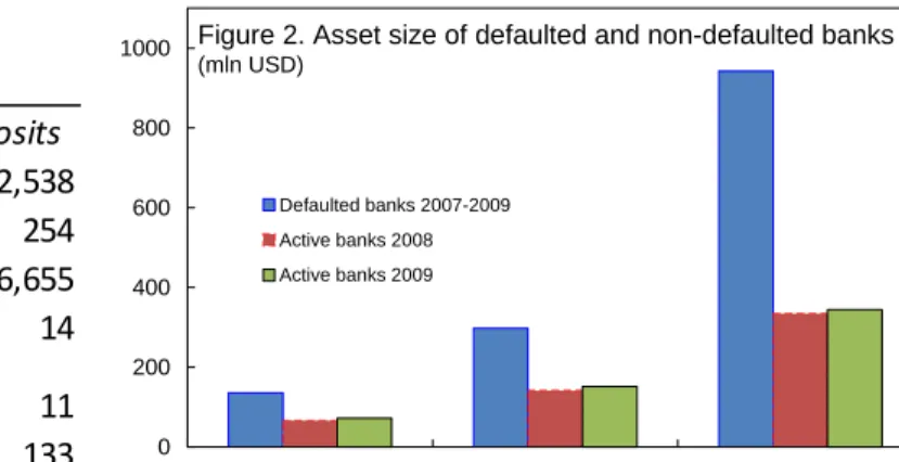
The 168 bank failures between 2007 and 2009 are distributed among relatively larger banks compared with the universe of active banks in 2008 and 2009. All quartiles of the distribution of the defaulted banks are higher than those of the entire population of active banks. The
9
statistics for the defaulted banks, referred to the year before default, are reported in Table 1 and Figure 2. Assets Deposits Mean 4,008 2,538 Median 297 254 Max 325,809 186,655 Min 14 14 Skewness 11 11 Kurtosis 138 133
Table 1. US bank failures 2007-2009: descriptive statistics (USD mn)
Source: FDIC, SNL Financials.
0 200 400 600 800 1000
1 Quartile Median 3 Quartile
Defaulted banks 2007-2009 Active banks 2008 Active banks 2009
Source: FDIC
Figure 2. Asset size of defaulted and non-defaulted banks
(mln USD)
For the purpose of the statistical analysis, a bank is considered defaulted in a given year t
based on the information released by the FDIC, provided that a balance sheet referred to the previous year t-1 is available. On a few occasions, when defaults occurred at the beginning of the calendar year t and the defaulting banks had not yet released their balance-sheet information for the period t-1,defaults were conventionally assigned to the previous calendar year t-1 so that a balance sheet existed one year before the default (i.e. at t-2).10
A paired sample of defaults and non-defaults was then selected for each given year from 2007 to 2009. Non-defaulted banks were selected from the entire universe of active banks by matching their asset size and year with that of the defaulted banks. After this procedure, the average asset size of the two paired sub-samples should not be, by construction, significantly different from one another. This null hypothesis is tested and accepted, with a t-test for paired samples (Table 2).
10
Sample
Average Asset Size at t-1 (USD mn)
Defaults 4,008
Non-defaults 4,847
One-tail t-test probability 16.15 Two-tails t-test probability 32.29 Table 2. Paired samples t-test: defaults and non-defaults 1/
1/ Non-sgnificance of the test statistic means that the null hypotesis of the two samples having the average is accepted.
The estimation sample therefore includes 336 banks, of which 168 failed over the period 2007–2009 and 168 were still going concerns at the end of the observation period (end-2009).
Using a matched sample is intuitively attractive compared with the use of the entire population, for which the estimates are affected by changes in the population characteristics and composition from one period to the next. By using a paired sample, the impact of these changes is avoided, reducing the volatility of the estimates. A low-default frequency potential problem is also addressed. However, the common sample has a reduced sample size and the sampling error can be partially offset by the reduced volatility on the matched sample estimates. More importantly, the sampling procedure does not ensure that the sample is representative of the population. This limitation can be overcome, however, by recalibrating the estimated model to the actual population, if need be, so that it can be used for forecasting purposes. In any case, this is not the immediate purpose of this work, for which the use of a paired sample appears desirable.
C. The Model
A Logit model is used to analyse the role of funding in explaining bank defaults. Logit regression models are applied very frequently in the field of credit risk to estimate probabilities of default because they have the advantage of being able to deal with dichotomous response variables, taking 0–1 values.11
In this work, as in much of the literature on credit and default risk, the binary dependent variable Si,t is a variable representing the status of bank i at time t. When Si,t =1 a bank is in default and when Si,t =0 a bank is a going concern.
11
As a first step in the model identification process, a base model of the likelihood of bank default is estimated. The model is based on a set of explanatory variables, which are intuitively related to the solvency conditions of a bank and which have consistently been shown in the existing literature to be significant predictors of banks’ likelihood of default.
A combination of bank-specific balance sheets and profit-and-loss variables as well as macro-economic variables has been selected, so that a satisfactory explanatory power is achieved while keeping the model efficient and limiting the number of variables used. The selection of the set of explanatory variables is based on both a statistical and a graphical analysis, always verifying the economic meaningfulness of each variable in order to include only those that would be acceptable not just from a statistical but also from an economic standpoint ex ante, and would show the expected sign ex post.12
Hence, only statistically significant variables with the correct signs have been selected in an iterative approach aimed at maximizing the log likelihood function of the model. The final specification has been identified through a two-step procedure: first the univariate predictive power of each variable has been assessed, and then the optimal multivariate specification has been identified. The variables chosen represent banks’ profitability, asset quality and capital adequacy and the interest rates prevailing in the market.
To address the non-existence of the explanatory variables for defaulted banks at time t, only lagged variables (with 1 to 4 lags) have been used in the process of model selection. The decision to use only lagged explanatory variables also limits the extent of any endogeneity issue in the model.
As a result, the following multivariate Logit model has been identified and estimated:
i t t t i t i t i t i NPL RBC ROAE PLR Size S , 1 2 ,13 ,14 ,15 2 6 1 ( 1 ) with Si,t being the status of each bank i at time t, NPLi,t-1, RBCi,t-1, ROAEi,t-1 being respectively the non-performing loans ratio, the risk-based capital ratio and the return on equity for bank i at time t-1, PLRt-2 being the level of the prime rate on short-term loans at time t-2 and Sizet-1the natural logarithm of the banks’ asset size at t-1 (Table 3).
The specification of the model described in equation (1) has been then amended to test for the hypothesis (i) and (ii) previously mentioned and, hence, to assess whether funding can be considered a meaningful indicator of banks’ risk conditions. In particular, variables representing bank funding conditions have been introduced.
12
The graphical analysis involves representing each variable on a scatter plot to see if there is an apparent separation of the values between the different statuses of default and non-default. However, this is not reported for parsimony.
The first augmented model aims in particular to test hypothesis (i) by using the loan-to-deposit ratio, LTDi,t, as explanatory variable, as specified by equation (2). This ratio provides a measure of the funding mix chosen by a bank to finance its loan portfolio. The higher the LTD ratio the less the bank is using customer deposits to finance its loan portfolio.
i t i t t i t i t i t i t i NPL RBC ROAE PLR Size LTD S, 12 .13 ,14 ,15 ,2 6 17 ,3 ( 2 ) If hypothesis (i) is correct, then a higher loan-to-deposit ratio should be positively related to banks’ riskiness and probability of default. It implies, in fact, that a larger share of bank assets is financed with forms of funding intrinsically more volatile than deposits.
Once the role of the composition of funding between deposits and non-deposits has been considered, an investigation of the role of different forms of deposits Di,k,t (with k being the different subset of deposits) is carried out to test hypothesis (ii). The alternative model specifications look at those deposits which, ex ante, can be considered potentially more volatile.
In particular, deposits that can be considered ex ante potentially less stable are those exceeding the level of coverage provided by the FDIC.13 Brokered deposits are also assessed
for the role they played in the S&L crisis. The time and non-time nature of deposits has been analysed as well. The variables used in the model are therefore the following:
- Brokered deposits to total deposits
- Deposits over $100,000 (or $250,000) to total deposits - Time deposits over $100,000 to total deposits
- Non-time deposits over $100,000 to total deposits - Non-time deposits to total deposits
The equation including the deposit variables listed above is the following.
i j t k i t t i t i t i t i t i NPL RBC ROAE PLR Size D S, 12 ,13 ,14 ,15 ,26 17 ,, ( 3 ) 13
The threshold used is $100,000 in line with the maximum coverage provided by the FDIC before the crisis. The limit, however, has been temporarily increased to $250,000 as of 3 October 2008 (Our usage and it avoids too many commas). On 20 May 2009, the temporary measure was extended to the end of 2013. On 21 July 2010, the approval of the Dodd-Frank Wall Street Reform and Consumer Protection Act permanently raised the maximum coverage to $250,000 (FDIC 2010a). On 9 November 2010, the FDIC issued a Final Rule implementing Section 343 of the Dodd-Frank Wall Street Reform and Consumer Protection Act that provides for unlimited insurance coverage of non-interest-bearing transaction accounts (FDIC 2010b).
D. Results
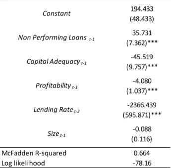
The basic results confirm the findings of the literature on bank defaults, which show clear evidence of the relationship between probability of default and capital adequacy, profitability and asset quality. These variables are all very significant in explaining bank defaults in the United States between 2007 and 2009 (Table 4).
Looking at the role of funding, the results also indicate clearly that funding played a key role in determining banks’ default risk. A weaker deposit base negatively affects the likelihood of bank failure. In particular, both the level and the composition of deposit funding appear to matter.
It is found that both the extent to which a bank is funding its asset through deposits (rather than other forms) and the intrinsic stability of the deposit base play a key role in explaining bank default. Both these dimensions are relevant for the sample analysed, after controlling for bank-specific variables (profitability, capitalization, asset quality and size) and macro-economic variables.
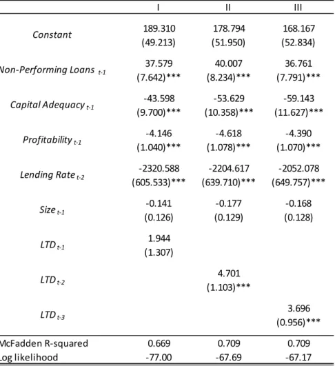
In particular, a higher level of the loan-to-deposit ratio or, in other words, a heavier reliance by banks on alternative forms of funding to deposits, significantly increases banks’ probability of default.14 Defaults are more likely not only immediately after a higher level of
the loan-to-deposit ratio is observed but also two to three years after such an increase. This implies that banks need to achieve a balanced funding position in a structural and stable manner, since temporary improvements in the funding profile (or temporary weakening) are not likely to affect banks’ stability in a significant way (Table 5).
Not all deposits, however, contribute equally to banks’ funding stability. Although results are subject to some uncertainties, they seem to suggest clearly that different types of deposits have different effects on banks’ likelihood of default, with the reliance on more volatile sources of deposits appearing to be a significant risk factor.
Deposits above the level of coverage provided by the deposit insurance scheme contribute, however, to explaining bank defaults in a specific way. While there is no apparent effect of the stock of deposits above the level of deposit insurance, there is still some indication that higher reliance on deposits above the level of coverage might imply a higher probability of default. In particular, deposits above the level of coverage and with time-nature appear to be correlated to the default risk (Table 6). This finding might indicate that when a bank’s conditions tend to deteriorate, the bank’s managers increase their preference for large time-deposits, possibly in the knowledge that their time feature will make them inherently more stable than large demand deposits if the bank’s conditions worsen.
14
Merrouche and Nier (2010) provide empirical evidence of the possible reasons behind the build-up of financial imbalances (as measured by the loan-to-deposit ratio) in OECD countries ahead of the global financial crisis.
Hardly anything can be said, however, for the entire stock of deposits above the level of coverage which, in this analysis, is non-significant in explaining bank default. There is in fact no clear evidence of more stringent bank monitoring by uninsured depositors that one would expect ex ante. However, the variable representing large demand deposits, although non-significant, shows a negative sign, suggesting some consistency with the hypothesis of more active monitoring by large demand depositors.
Brokered deposits are still a significant variable in explaining bank defaults, despite the regulatory limitations introduced after the S&L crisis. Higher levels of brokered deposits are in fact significantly associated with higher default probabilities. Such a relation appears to be stable and persistent, provided that the significance of this variable is observed from one to three periods before default. Hence, it can be argued that the more persistently problematic institutions tend to rely more than sound institutions on such a form of funding without being able to achieve any improvement in their funding conditions, but rather further increase their default risk. The effectiveness of the regulations introduced after the S&L crisis appears questionable.
Overall, banks’ management actions seem to signal weak conditions better than depositors’ monitoring efforts. With the variables approximating the latter not being significant, the variables most likely to reflect banks’ managerial actions, such as time-deposits and brokered deposits, show a much clearer relationship with the banks’ probability of default.
However, in either case it is evident that the banks’ funding choices do affect their probability of default and clearly indicate deteriorating conditions well ahead of the actual failure.
18
Table 4. Basic determinants of bank defaults 1/ 194.433 (48.433) 35.731 (7.362)*** -45.519 (9.757)*** -4.080 (1.037)*** -2366.439 (595.871)*** -0.088 (0.116) McFadden R-squared 0.664 Log likelihood -78.16
*** Shows significance at 1 per cent.
Lending Ratet-2
Constant
Non Performing Loans t-1
Capital Adequacyt-1
Profitabilityt-1
Sizet-1
1/ Dependent variable is bank status (default/non-default).
Variable Name Bank status (S) Non-performing loans (NPL) Capital adequacy (RBC) Profitability (ROAE) Lending rate (PLR) Size LTD Brokered deposits Large time deposits Large non-time deposits All large deposits All non-time deposits
average prime rate on short-term loans to business
loan-to-deposit ratio
Source: Board of Governors of the Federal Reserve System, FDIC, SNL Financials, US Bureau of Economic Analysis, US Bureau of Labor Statistics.
deposits above $ 100.000 to total deposits
1/ A bank is considered to be in default when US authorities intervene and it is included in the list of failed banks by the FDIC.
non-time deposits to total deposits natural logarithm of the bank's total asset size
brokered deposits to total deposits Time deposits above $ 100.000 to total deposits non time-deposits above $ 100.000 to total deposits
return on average equity Table 3. Definition of variables used in the main model
Definition
non-performing loans to total gross loans risk-based captial ratio
default/non-default 1/
19 189.310 178.794 168.167 (49.213) (51.950) (52.834) 37.579 40.007 36.761 (7.642)*** (8.234)*** (7.791)*** -43.598 -53.629 -59.143 (9.700)*** (10.358)*** (11.627)*** -4.146 -4.618 -4.390 (1.040)*** (1.078)*** (1.070)*** -2320.588 -2204.617 -2052.078 (605.533)*** (639.710)*** (649.757)*** -0.141 -0.177 -0.168 (0.126) (0.129) (0.128) 1.944 (1.307) 4.701 (1.103)*** 3.696 (0.956)*** McFadden R-squared 0.669 0.709 0.709 Log likelihood -77.00 -67.69 -67.17
1/ Dependent variable is bank status (default/non-default). *** Shows significance at 1 per cent.
II III LTDt-2 LTDt-3 Sizet-1 Non-Performing Loans t-1 Capital Adequacyt-1 Profitabilityt-1 Lending Ratet-2 LTDt-1 Constant
Table 5. Introducing funding. The impact of the loan-to-deposit ratio on bank defaults 1/
20
IX Table 6. Bank defaults. Does deposit composition matter? Looking at size, contractual maturity (demand vs time ), and brokered 1/
I II III IV V VI VII VIII
195.427 182.051 185.400 167.756 149.028 148.922 193.524 187.291 194.068 (50.358) (49.817) (50.159) (50.325) (53.645) (52.834) (48.326) (49.197) (48.460) 35.563 34.476 35.202 37.464 33.301 29.03 36.426 35.086 35.726 (7.630)*** (7.567)*** (7.484)*** (7.813)*** (7.792)*** (7.702)*** (7.519)*** (7.396)*** (7.357)*** -39.705 -40.574 -39.984 -43.678 -45.257 -43.704 -45.835 -44.477 -45.717 (9.673)*** (9.595)*** (9.686)*** (9.843)*** (10.805)*** (12.141)*** (9.837)*** (9.699)*** (9.912)*** -4.122 -4.209 -4.085 -4.044 -4.054 -3.579 -4.081 -4.071 -4.086 (1.040)*** (1.053)*** (1.051)*** (1.034)*** (1.031)*** (1.201)*** (1.045)*** (1.023)*** (1.038)*** -2394.988 -2222.935 -2263.046 -2059.617 -1803.660 -1797.489 -2357.988 -2280.533 -2362.963 (620.412)*** (613.178)*** (617.108)*** (619.162)*** (660.756)*** (652.023)*** (594.765)*** (605.0989)*** (595.816)*** -0.084 -0.100 -0.103 -0.036 -0.142 -0.187 -0.099 -0.050 -0.083 (0.120) (0.119) (0.118) (0.123) (0.136) (0.146) (0.117) (0.122) (0.123) 4.335 (1.527)*** 5.413 (2.084)*** 3.644 (2.032)* 5.099 (2.088)** 4.415 (2.127)** 4.705 (1.927)** 0.876 (1.304) -1.640 (1.388) 0.457 (3.556)
All Large Depositst-1
Large Non-Time Depositst-1
All Non-Time Depositst-1
Brokered Depositst-1
Brokered Depositst-2
Brokered Depositst-3
Large Time Depositst-1
Large Time Depositst-2
Large Time Depositst-3
Profitabilityt-1 Lending Ratet-2 Constant Non-Performing Loans t-1 Capital Adequacyt-1 Sizet-1
E. Robustness
The Logit model presented above has been tested for robustness to the use of an alternative set of explanatory variables. First, a number of macroeconomic variables have been tested in alternative specifications of the model by replacing the lending rate previously used (the average prime rate on short-term loans to business) with the GDP growth rate, the unemployment rate, the consumer price index and an alternative measure of the lending rate (the conventional mortgage rate) (Table 7).
The unemployment rate and the alternative lending rate are shown to be significant and their introduction confirms the general findings of the main model specification presented above. GDP growth rate and CPI are also significant, but the former presents a sign that is not consistent with the economic rationale, while the interpretation of the latter is not immediate due to the unclear ex ante relationship between CPI and banks’ probability of default. Even in these cases, however, the funding variables remain highly significant, confirming the robustness of the estimates (Table 8).
The robustness of the results concerning the sensitivity of the banks’ probability of default to their funding conditions is also confirmed when using a different set of bank-specific variables to represent capital adequacy, profitability and asset quality. In practice, the tangible common equity ratio, net income before taxes to total assets, and provisions to total assets are now used instead of the risk-based capital ratio, the return on average equity and the non-performing loans ratio (Table 7). The results show that in all cases there is no loss of significance of the funding variables (Table 9).
This is also confirmed when jointly substituting the banks’ specific variables and the macroeconomic variable. In this last specification of the alternative model, all but one (bank size) of the control variables have been replaced from the original model and all three significant funding variables still retain, and even improve, their level of significance (Table 9). The difference here is that with the alternatively specified set of bank-specific variables the bank size variable, which was previously never significant, now becomes somewhat significant.
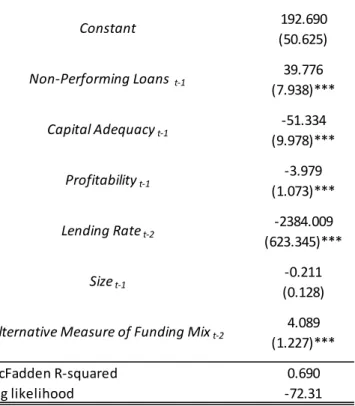
The results are also robust to the use of alternative specifications of the banks’ funding mix. While in the main model the LTD ratio has been used as the best performing proxy for funding composition, alternative variables could also have been used to measure the bank funding mix. To verify the robustness of results to this choice a commonly used alternative to the LTD ratio, the assets-to-deposits ratio, has also been tested. Results show that the assets-to-deposits ratio is as significant as the LTD ratio in explaining banking crises (Table 10).
22 Variable Name Asset Quality Capital Adequacy Profitability GDP Inflation Rate Unemplyment Rate
GDP Growth Rate, Real (Percentage Change) CPI-U Non-Seasonally Adjusted
Definition Provisions to Total Assets
Tangible Common Equity Ratio
Source: Board of Governors of the Federal Reserve System, SNL Financials, US Bureau of Economic Analysis, US Bureau of Labor Statistics.
Unemployment Rate Seasonally Adjusted Table 7. Definition of bank-specific and macroeconomic variables used in the alternative models
Net Income Before Taxes to Total Assets
Contract Rate on 30Y Fixed Rate Conventional Home Mortgage Commitments
25.803 28.927 25.305 -13.904 -14.720 -13.342 0.677 1.650 1.122 0.773 1.803 1.220 (7.259) (6.964) (7.009) (4.122) (3.956) (3.929) (1.951) (1.885) (1.991) (1.949) (1.897) (1.999) 39.770 35.580 37.683 39.996 36.090 38.081 39.972 35.964 38.011 39.221 34.775 36.920 (8.104)*** (7.512)*** (7.760)*** (8.056)*** (7.554)*** (7.742)*** (8.117)*** (7.570)*** (7.800)*** (8.027)*** (7.376)*** (7.634)*** -50.537 -36.519 -39.978 -49.939 -36.068 -39.936 -50.480 -36.598 -40.135 -50.319 -36.031 -39.459 (9.915)*** (9.078)*** (9.199)*** (9.825)*** (9.204)*** (9.288)*** (9.906)*** (9.143)*** (9.261)*** (9.878)*** (8.956)*** (9.069)*** -4.284 -3.812 -3.701 -4.261 -3.854 -3.745 -4.309 -3.869 -3.746 -4.192 -3.682 -3.595 (1.037)*** (0.997)*** (0.990)*** (1.032)*** (1.005)*** (0.996)*** (1.040)*** (1.005)*** (0.996)*** (1.027)*** (0.979)*** (0.979)*** -0.177 -0.067 -0.026 -0.185 -0.089 -0.045 -0.079 -0.037 -0.159 -0.044 -0.006 (0.124) (0.114) (0.115) (0.123) (0.114) (0.116) (0.114) (0.115) (0.123) (0.114) (0.115) -385.297 -418.459 -371.129 (102.646)*** (99.060)*** (98.573)*** 343.454 387.485 342.466 (92.324)*** (88.420)*** (87.927)*** 120.945^ 133.871 ^ 118.285 ^ (31.917)*** (30.963)*** (30.643)*** 52.035 ^ 54.823 ^ 48.758 ^ (14.332)*** (13.639)*** (13.719)*** 4.618 4.580 4.585 4.696 (1.061)*** (1.049)*** (1.057)*** (1.066)*** 4.275 4.483 4.352 4.171 (1.496)*** (1.510)*** (1.505)*** (1.481)***
Large Time Depositst-1 4.767 4.957 4.782 4.815
(2.006)** (1.975)** (1.998)** (2.010)**
McFadden R-squared 0.694 0.665 0.658 0.692 0.659 0.659 0.695 0.667 0.660 0.692 0.660 0.654
Log likelihood -71.21 -78.01 -79.38 -71.64 -79.15 -79.16 -71.11 -77.59 -79.05 -71.81 -79.15 -80.31
1/ Dependent variable is bank status (default/non-default). *, **, *** Show significance at 10, 5 and 1 per cent respectively.
^ Indicates that the sign is either not the expected one or its interpretation is not univocal.
I d Table 8. Bank defaults and funding relevance. Testing for robustness to alternative macroeconomic variables 1/
III c II d III d III a I b I c II c Sizet-1 II a Constant III b Non-Performing Loans t-1 Capital Adequacyt-1 Profitabilityt-1 I a II b Brokered Depositst-1 CPIt-1
Alternative Lending Ratet-3
Unemployment Ratet-3
LTDt-2
240.970 260.263 234.210 -12.487 -13.227 -12.656 (55.013) (57.914) (55.357) (4.276) (4.325) (4.161) -1.147 -1.038 -1.201 -1.233 -1.183 -1.339 (0.376)*** (0.385)*** (0.383)*** (0.370)*** (0.399)*** (0.391)*** -72.493 -63.215 -66.283 -70.635 -60.386 -64.505 (12.116)*** (11.287)*** (11.415)*** (11.944)*** (11.032)*** (11.203)*** -44.558 -43.112 -40.968 -43.451 -41.482 -39.801 (8.752)*** (8.457)*** (8.301)*** (8.617)*** (8.311)*** (8.197)*** -0.386 -0.299 -0.228 -0.382 -0.295 -0.223 (0.134)*** (0.127)** (0.125)* (0.131)*** (0.125)** (0.122)* -2913.715 -3136.585 -2827.246 (674.711)*** (710.410)*** (678.386)*** 427.962 474.537 435.971 (101.286)*** (103.617)*** (99.986)*** 4.092 4.580 (1.103)*** (1.049)*** 5.385 5.322 (1.566)*** (1.543)***
Large Time Depositst-1 6.155 6.243
(2.006)*** (2.223)***
McFadden R-squared 0.633 0.623 0.608 0.623 0.613 0.600
Log likelihood -82.35 -84.57 -87.66 -84.49 -86.84 -89.53
1/ Dependent variable is bank status (default/non-default). *, **, *** Show significance at 10, 5 and 1 per cent respectively.
I b II b
Constant
I a II a III a III b
LTDt-2
Brokered Depositst-1
Table 9. Bank defaults and funding relevance. Testing for robustness to alternative bank-specific variables 1/ Alternative Profitability t-1 Sizet-1 Lending Ratet-3 Unemployment Ratet-3 Alternative Capital Adequacy Ratio t-1
Alternative Asset Quality Ratio t-1
192.690 (50.625) 39.776 (7.938)*** -51.334 (9.978)*** -3.979 (1.073)*** -2384.009 (623.345)*** -0.211 (0.128) 4.089 (1.227)*** McFadden R-squared 0.690 Log likelihood -72.31
1/ Dependent variable is bank status (default/non-default). *** Shows significance at 1 per cent.
Alternative Measure of Funding Mixt-2
Constant
Non-Performing Loans t-1
Sizet-1
Table 10. Testing for robustness of results to an alternative measure of funding mix 1/
Capital Adequacyt-1
Profitabilityt-1
V. CONCLUSIONS
The experience of the latest financial crisis has shown how crucial liquidity conditions can be for banks’ operations under stress and their likelihood of survival. For medium and large banks in particular, critical liquidity conditions can spill over to other parts of the financial system, with negative consequences on stability. The evidence of this paper confirms that funding liquidity conditions significantly affect banks’ risk profile and, ultimately, their likelihood of default.
The empirical evidence for US banks therefore provides clear support for more careful regulation and supervision of banks’ liquidity conditions by the supervisory and regulatory authorities. While this paper focuses on US banks only, the policy recommendation of tighter regulation and supervision of liquidity conditions can arguably be extended to a large number of countries.
The evidence of the relationship between banks’ funding profiles and their risk of default can be related to the new regulatory framework for liquidity risk adopted by the Basel Committee on Banking Supervision (2010). While the main purpose of the paper is neither to assess the new framework nor to discuss the optimal design of liquidity regulation, it is possible, however, to note that the new rules appear to have the potential and the features to help reduce the likelihood of banks’ experiencing liquidity weaknesses.16 In particular, by differentiating the treatment for
the more stable and the less-stable deposits in the context of both the liquidity coverage ratio and the net stable funding ratio, the regulatory framework correctly recognizes the different impacts that different deposits can have on banks’ stability. Nevertheless, the implementation of the new measures will be of great importance, as supervisory authorities will be called upon to identify those deposits that are more likely to have a destabilizing effect on banks.
It will be also important that the new regulation be applied extensively within and across banking systems. The findings of this analysis in fact suggest that it is advisable not to limit the application of the new liquidity regulations only to internationally active banks, but rather to extend their application also to medium- and small-sized institutions, whose survival too can be critically affected by a weak liquidity and funding profile.
The US authorities might also wish to reconsider the existing regulation on the use of brokered deposits, which does not appear to have been effective enough in reducing their abuse, as this remains a critical factor in explaining defaults of US banks.
Finally, while the introduction of prudential regulation on liquidity appears important, it is also essential for this to be combined with reinforced supervisory focus on the specific risk area, which was almost completely neglected by supervisory authorities worldwide ahead of the crisis.
16
Perotti and Suarez (2011) analyse the design of liquidity regulation and suggest that an optimal policy should involve both price and quantity rules.
REFERENCES
Acharya V.V., Gale D. and Yorulmazer, T. (2008). Rollover Risk and Market Freezes. Working Paper, NYU Stern.
Altman E. I. (1977). Predicting Performance in the Savings and Loan Association Industry.
Journal of Monetary Economics, 3(4), 443–66.
——— (1981). Application of Classification Techniques in Business, Banking and Finance. Contemporary Studies in Economic and Financial Analysis, 3. Greenwich, CT:
JAI Press Inc.
Barth J. R., Bartholomew P. and Labich, C. (1990). Moral Hazard and the Thrift Crisis: An Analysis of 1988 Resolutions. Consumer Finance Law Quarterly Report, Winter 1990. Basel Committee on Banking Supervision. (2010). Basel III: International Framework for
Liquidity Risk Measurement, Standards, and Monitoring, December 16, 2010.
Berger A.N., and Turk-Ariss R. (2011). Do Depositors Discipline Banks: an International Perspective. Unpublished.
Billet M., Garfinkel J., and O’Neal E. (1998). The Cost of Market Versus Regulatory Discipline in Banking. Journal of Financial Economics, 48, 333–358.
Bologna P. (2010). Australian Banking System Resilience: What Should Be Expected Looking Forward? An International Perspective. IMF Working Paper, WP/10/228.
——— Hardy D., Ivanova A. and Sodsriwiboon P. (2011). Germany: Banking Sector Structure. IMF Technical Note, unpublished.
Bongini P., Claessens S. and Ferri, G. (2001). The Political Economy of Distress in East Asian Financial Institutions. Journal of Financial Services Research, 19(1), 5–25.
Bruche M. and Suarez J. (2010). Deposit Insurance and Money Market Freezes. Journal of Monetary Economics, 57(1).
Calomiris C. and Kahn C. (1991). The Role of Demandable Debt in Structuring Optimal Banking Arrangements. American Economic Review, 81, 497–513.
———Building an Incentive-Compatible Safety Net. Journal of Banking and Finance, 23(10), 1499–1519.
Cole R. A. and Gunter J.W. (1995). Separating the Likelihood and Timing of Bank Failure.
Journal of Banking and Finance, 19(6), 1073–1089.
——— and Wu Q. (2009). Is Hazard or Probit More Accurate in Predicting Bank Failures? Paper presented at the 22nd Australasian Finance and Banking Conference
(December 15–17) and at the Federal Deposit Insurance Corporation Research Seminar (May 19).
——— and White L.J. (2010). Déjà Vu All Over Again: The Causes of the U.S. Commercial Bank Failures This Time Around. Presentation at the 2010 Federal Deposit Insurance Corporation Research Conference (October 28).
Cook D. and Spellman L. (1994). Repudiation Risk and Restitution Costs: Toward Understanding Premiums on Insured Deposits. Journal of Money Credit and Banking, 26(3), 439–459.
Davison L. (2000). Banking Legislation and Regulation. In Hanc G. (ed.). Histories of the 80s. i:
An Examination of the Banking Crises of the 1980s and Early 1990s. Washington D.C.: Federal Deposit Insurance Corporation.
Demirgüç-Kunt A. and Detragiache E. (1998). The Determinants of Banking Crises in Developing and Developed Countries. IMF Staff Papers, 45, 81–109.
——— and Detragiache E. (2002). Does Deposit Insurance Increase Banking System Stability? An Empirical Investigation. Journal of Monetary Economics, 49(7), 1373–1406.
Demyanyk Y. and Hasan I. (2009). Financial Crises and Bank Failures: A Review of Prediction Methods. Bank of Finland Research Discussion Papers, 35/2009.
Dewatripont M. and Tirole J. (1994). The Prudential Regulation of Banks. Boston: Massachusetts Institute of Technology.
Diamond D. and Dybvig P. (1983). Banks Runs, Deposit Insurance, and Liquidity. Journal of Political Economy, 91, 201–419.
——— and Rajan R. (2001). Banks, Short Term Debt and Financial Crises: Theory, Policy, Implications and Applications. Carnegie-Rochester Conference Series on Public Policy, 54, 37–31.
Federal Deposits Insurance Corporation. (2010a). Basic FDIC Insurance Coverage Permanently Increased to $250,000 Per Depositor. FDIC Press Release, July 21.
Federal Deposits Insurance Corporation. (2010b). Final Rule: Temporary Unlimited Coverage for Noninterest-Bearing Transaction Accounts. Financial Institution Letter,November 9.
Flannery M.J. (1994). Debt Maturing and the Deadweight Cost of Leverage: Optimally Financing Banking Firms. American Economic Review, 84(1), 320–331.
——— (1998). Using Market Information in Prudential Bank Supervision: A Review of the U.S. Empirical Evidence. Journal of Money Credit and Banking, 30, 273–305.
Gilbert R.A. and Vaughan M.D. (2001). Do Depositors Care About Enforcement Actions?
Goldberg L. and Hudgins S. (1996). Response of Uninsured Depositors to Impending SandL Failures: Evidence of Depositors’ Discipline. Quarterly Review of Economics and Finance, 36(3), 311–325.
——— and Hudgins S. (2002). Depositor Discipline and Changing Strategies for Regulating Thrift Institutions. Journal of Financial Economics, 63(1), 263–274.
Goldsmith-Pinkham P. and Yorulmazer T. (2010). Liquidity, Bank Runs and Bailouts: Spillover Effects During the Northern Rock Episode. Journal of Financial Services Research, 37 (2-3), 83–89.
Gonzales-Hermosillo B. (1999). Determinants of Ex Ante Banking System Distress: a Macro-Micro Empirical Exploration. IMF Working Paper, 99/33. Washington D.C.: International Monetary Fund.
——— and Ratnovski L. (2011). The Dark Side of Bank Wholesale Funding. Journal of Financial Intermediation, 20(2), 248–263.
Greene W.H. (2011). Econometric Analysis. 6th edn. Prentice Hall.
Gujarati D. N. (1995). Basic Econometrics. 3rd edn. Singapore: McGraw-Hill International Edition – Economic Series.
Huang R. and Ratnovski L. (2009). Why Are Canadian Banks More Resilient? IMF Working Paper, 09/152. Washington D.C.: International Monetary Fund.
Jagtiani J. and Lemieux C. (2001). Market Discipline Prior to Failure. Journal of Economics and Business, 53, 283–311.
Jordan J., Peek J. and Rosengren E. (1999). The Impact of Greater Banks Disclosure Amidst Banking Crises. Federal Reserve Bank of Boston Working Paper, 99–1.
Lane W. R., Loonoey S. W. and Wansley J. W. (1986). An Application of the Cox Proportional Hazard Model to Bank Failure. Journal of Banking and Finance, 10(4), 511–531.
Martin D. (1977). Early Warning on Bank Failure: a Logit Regression Approach. Journal of Banking and Finance, 1(3), 249–276.
Merrouche O. and Nier E. (2010). What Caused the Global Financial Crisis? Evidence on the Drivers of Financial Imbalances 1999–2007. IMF Working Paper, 10/265. Washington D.C.: International Monetary Fund.
Moore R.R. (1991). Brokered Deposits: Determinants and Implications for Thrift Institutions.
Federal Reserve Bank of Dallas Financial Industry Studies, December.
Park S. and Peristiani S. (1998). Market Discipline by Thrift Depositors. Journal of Money Credit and Banking, 30(3), 347–365.
Perotti E. and Suarez J. (2011). A Pigovian Approach to Liquidity Regulation. Tinbergen Institute Discussion Paper, 11-040/2/DSF15.
Pifer H.W. and Meyer P.A. (1970). Prediction of Bank Failures. Journal of Finance, 25(4), 853– 868.
Shin H.S. (2009). Reflections on Northern Rock. Journal of Economic Perspectives, 23(1), Winter 2009, 101–111.
Sinkey J. F. (1975). A Multivariate Statistical Analysis of the Characteristics of Problem Banks.
Journal of Finance, 30(1), 21–36.
——— and Pettaway R. H. (1980). Establishing On-Site Bank Examination Priorities: an Early Warning System Using Accounting and Market Information. Journal of Finance, 35(1), 137–150.
van der Ploeg S. (2010). Bank Default Prediction Models: a Comparison and an Application to Credit Rating Transitions. Erasmus University Rotterdam. Unpublished.
Viñals J., Fiechter J., Pazarbasioglu C., Kodres L., Narain A. and Moretti M. (2010). Shaping the New Financial System. IMF Staff Position Note, October 3, 2010, SPN/10/15.
Whalen G. (1991). A Proportional Hazard Model of Bank Failure: An Examination of its Usefulness as an Early Warning Tool. Economic Review, 27(1), 21–31. Cleveland: Federal Reserve of Cleveland.
Wheelock D.C. and Wilson P.W. (2000). Why Do Banks Disappear? The Determinants of U.S. Banking Failures and Acquisitions. Review of Economics and Statistics, 82(1), 127–138.