Openness and Inflation
∗Dudley Cooke†
University of Essex
Abstract: A general equilibrium model of a small open economy is developed to analyze the optimal rate of inflation under discretion. Once agents’ welfare is the sole policy objective it is possible to show that openness and inflation no longer have a simple inverse relationship. A greater degree of openness may lead the policy maker to want to exploit the short-run Phillips curve more aggressively, even if involves a smaller short-run benefit, because changes in export demand affect the terms of trade. Inflation can then be higher in a more open economy.
JEL Classification: E31, E52, F41.
Keywords: Inflation bias, terms of trade, export demand, small open economy.
∗I thank Martin Ellison, Philip Lane and Neil Rankin for helpful comments. Suggestions from seminar
participants at City University, Carlos III, Korea University, Sveriges Riksbank, Warwick and UCL have also helped the development of the paper. Financial support from the ESRC (#R42200134107) is gratefully acknowledged.
†Department of Economics, University of Essex. Wivenhoe Park, Colchester CO4 3SQ, Essex, UK.
1. Introduction
Will inflation rise or fall as an economy becomes more open? One way to approach this question is through the time inconsistency problem of monetary policy.1 Typically, the
answer is that inflation is lower in an open economy because deteriorations in the terms of trade increase the costs of surprise monetary expansions. As an economy becomes more open, the terms of trade effect becomes stronger, the associated costs greater, and inflation lower.2 However, this result is generated using a postulated loss function. I
develop a general equilibrium model of a small open economy to analyze the optimal rate of inflation under discretion. When the maximization of agents’ welfare is the sole policy objective it is possible to provide a simple explanation of why inflation may rise or fall as an economy becomes more open.
Determining the rate of inflation under discretion in a general equilibrium setting rests on the introduction of the costs and benefits of expansionary monetary policy. Previous work studying the welfare implications of monetary policy in open economies, such as Obstfeld and Rogoff (1995), Corsetti and Pesenti (2001) and Benigno (2002), does not incorporate an explicit welfare cost of current inflation. As a result it is not possible to generate a time-consistent (discretionary) equilibrium.3 One contribution of this paper is
to introduce such a welfare cost, in a relatively simple way, and so bring about the existence of a time-consistent equilibrium. This makes it possible to study the relationship between openness and inflation in detail.
In the analysis presented below, a direct cost to current inflation is introduced by assuming beginning-of-period real money balances directly enter the utility function. Households are then required to make a money holding decision before production and consumption decisions.4 Inflation is costly because it reduces purchasing power. The welfare benefits
1For example, see Rogoff’s (1985) Mundell-Fleming extension of Barro and Gordon’s (1983) analysis. 2Romer (1993) and Lane (1997) provide a starting point for the empirical analysis of this relationship.
Both of these studies suppose it is the inability of the government to commit to a policy action that determines the rate of inflation.
3Benigno (2002) can, in fact, generate a time-consistent equilibrium as a special case. The result
relies on some specific values for the structural parameters of the model.
worker-of inflation occur through increases in an inefficiently low level worker-of output. This is captured by supposing that labor is supplied in a monopolistically competitive market and that there are one period nominal wage rigidities. The costs and benefits of surprise inflation are introduced in this way for two reasons. First, even in an open economy, it allows the derivation of an explicit expression for inflation without linear approximations. Second, without sacrificing internal consistency, the assumptions help capture the type of results found using reduced-form models, allowing for some interesting comparisons.
The results show that openness alters inflation via two main mechanisms. First, there is a standard effect which operates through the Phillips curve; when an economy is more open the slope of the Phillips curve is steeper, increasing the inflation cost and reducing the output gain from a surprise monetary expansion. There is a second effect present, however, because export demand interacts with openness and this affects the terms of trade. For a given degree of openness, an increase in export demand improves the terms of trade. This creates a larger incentive for the government to inflate because more favorable terms of trade imply a one unit increase in output leads to a bigger increase in consumption and a larger utility gain. As a result, export demand also influences the openness-inflation relationship. If export demand is sufficiently high, a greater degree of openness may lead the policy maker to exploit the short-run Phillips curve, even if it involves a smaller short-run benefit from doing so. In a rational expectations equilibrium, inflation can then be higher in a more open economy, in contrast to the standard result. There is a related literature that focuses on discretionary monetary policy in a dynamic general equilibrium setting. Perhaps the most well known approach is Woodford’s (2003) cashless linear-quadratic analysis, in which a cost to inflation is introduced through the use of a staggered pricing structure similar to Calvo (1983). Because only a fraction of firms are allowed to re-optimize their price in response to a shock, the costs of expansionary policy (or rather positive levels of inflation) are associated with relative price distortions across goods.5 This approach has been extended to a two country framework by Clarida shopper argument used to motivate both CIA and MIU models. The specification used here can also be thought of as implying a precautionary demand for money. This approach has been adopted in Danthine and Donaldson (1986), Neiss (1999) and most recently Perrsonet al. (2006).
et al. (1999, 2002), Benigno and Benigno (2003) and Pappa (2004) to incorporate terms of trade effects. In all of these papers the benefits of expansionary monetary policy occur because of monopolistic competition and nominal rigidities.
A second approach, more related to this paper, is taken by Albanesiet al. (2003). In this case, a cost to current inflation is introduced by assuming that households use previously accumulated cash to buy a subset of goods consistent with Svensson’s (1985) timing change. Higher realized inflation then forces households to substitute towards non-cash goods, which lowers welfare. However, inflation also raises output because some prices are fixed. This reduces the monopoly distortion and raises welfare, generating a policy trade-off. Arseneau (2004) analyzes a two country model with a cash-in-advance constraint. Following Ireland (1997), he assumes there is an upper bound to the rate of money growth to generate a discretionary outcome. Interestingly, both Albanesi et al. and Arseneau show that there can be multiple discretionary Markov equilibria.6 This paper shows that
there is either an interior solution on no solution, depending on an interplay between openness and the monopoly distortion.
The remainder of the paper is organized as follows. In section two I describe the model economy. In section three I solve the model for an arbitrary rate of money growth. Section four computes the discretionary rate of inflation and looks in detail at it’s relationship with openness. Section five concludes.
2. Model Economy
There are two economies - domestic and foreign. Both consist of a continuum ofj ∈[0,1] households which supply a differentiated labor type, hold real money balances and nominal bonds and consume domestic and foreign goods. Firms produce a single specialized output using labor as the input. The government controls the supply of money through lump-sum transfers. The foreign economy is assumed to be large relative to the domestic economy implying that the domestic economy takes financial conditions in the foreign economy as given and that domestic exports form a negligible component of the foreign
of the LQ approach in the context of discretionary monetary policy making.
6Multiple discretionary equilibria also arise in Armenter and Bodenstein’s (2005) analysis of a model
economy’s consumption basket. Consumption, output and the nominal price of the domestic output are denoted with h-subscripts and for foreign consumption, output and prices f is used. Asterisks denote foreign economy variables.
2.1. Firms
Firms maximize profits, ϑt(j) =Ph,tyt−
R1
0 wt(j)lt(j)dj, choosing amongst differentiated
labor types, lt(j), subject to a constant elasticity of substitution production function,
yt= µZ 1 0 lt(j)(σ−1)/σdj ¶σ/α(σ−1) (1) where wt(j) is the jth individuals nominal wage, Ph,t is the GDP deflator, yt domestic
output, α > 1 measures the returns to scale in production, and σ > 1 measures the elasticity of input substitution. Conditional labor demand is,
lt(j) = (wt(j)/wt)−σytα (2)
where wt=
³R1
0 wt(j)1−σdj
´1/(1−σ)
is the wage index. Since all households set the same wage in equilibrium, final labor demand is given by,
yt= (αwt/Ph,t)1/(1−α) (3)
In an open economy, output depends on the GDP deflator. It is possible to setα= 1, but with predetermined nominal wages, the GDP deflator will also be predetermined such that the domestic component of the inflation rate will be independent of monetary surprises.7
2.2. Households
Suppressing the j index, household utility is,
U0 =
∞
X
t=0
βt[lnCt+υ(mt)−φlκt/κ] (4)
7In a closed economyα6= 1 is a necessary assumption for the overall price level not to be predetermined
when there is nominal wage rigidity. In an open economy the overall price may vary through changes in the exchange rate.
where consumption, Ct, is Cobb-Douglas index of domestic and foreign goods; Ch,t and
Cf,t respectively.
Ct≡Ch,tn Cf,t1−n/nn(1−n)1−n
The υ(mt) term captures the liquidity services of real money balances, mt ≡ Mt/Pt,
where Pt is the consumer price index (CPI), and is assumed to be strictly increasing and
strictly concave. Finally,lt is labor supply. The parameter nis a measure of the degree
of openness, β ∈(0,1) is the discount factor, φ >0 is a weight attached to the disutility of labor and 1/(1−κ) is the elasticity of labor supply, withκ >1.
Households maximize utility choosing a sequence of nominal bond and domestic nomi-nal money holdings, consumption, and a desired wage rate, subject to the sequence of constraints,
Bt+Mt+1 =ϑt+wtlt−Ph,tCh,t−Pf,tCf,t+Tt+Bt−1(1 +it−1) +Mt (5)
and conditional labor demand, where Bt are bonds denominated in domestic currency
which pay a nominal net rate of interest it and Tt are lump-sum transfers.
The optimal allocation of expenditure between domestic and imported goods is,
Ch,t =nPtCt/Ph,t and Cf,t= (1−n)PtCt/Pf,t (6)
where Pt ≡ Ph,tn Pf,t1−n, and total consumption expenditures by domestic households are
therefore Ph,tCh,t+Pf,tCf,t =PtCt. The following conditions also hold for all t≥0,
Pt+1Ct+1 =PtCtβ(1 +it) (7)
wt=σφPtCt/(σ−1)l1t−κ (8)
υ0(mt+1) =Ct+1/it (9)
where υ0(mt+1) is the derivative ofυ(mt+1). Equation (7) is the standard consumption
Euler equation. Equation (8) describes labor supply and includes the monopoly markup-up, σ/(σ −1), and the CPI. Once a rigid nominal wage is assumed labor is demand determined in the short-run because agents are always willing to supply more labor given
the existence of monopoly profits. Equation (9) expresses the demand for money. This expression is non-standard and reflects the assumption that money holdings are effectively chosen in periodt−1, and soMtis predetermined in periodt. Expansionary policy raises
the price level and this implies a utility cost in terms of forgone real balances.
The foreign economy is identical. But as it becomes infinitely large relative to the domestic economy the proportion of domestic goods in it’s consumption basket diminishes. That is, n∗ → 0, so that C∗
t ∼= Cf,t∗ and Pt∗ ∼= Pf,t∗ , which is normalized to unity as it is
exogenous. However, this does not mean export demand is zero since C∗
t itself is large.
Defining the inverse terms of trade as ρt≡Pf,t/Ph,t, as the law of one price holds for the
domestic good (i.e. Ph,t = stPh,t∗ ), foreign consumption of domestic production is given
by,
C∗
h,t =g∗tρt (10)
The composite variable g∗
t ≡n∗Ct∗ is a measure of export demand and is exogenous from
the viewpoint of the domestic economy.8
2.3. Government
The government’s budget constraint is given by the following.
Tt =Mt+1−Mt (11)
Now all the constraints have been introduced it is clear how the beginning-of-period real money balances assumption works. Because period t nominal money holdings are predetermined, a monetary expansion in period t is not an increase in Mt, rather Mt+1
increases, and this produces the increase in Pt. This explains how surprise inflation in
period t unambiguously reduces current real money balances. 2.4. Equilibrium
8PPP does not hold since there is a form of consumption home bias, that is,n 6=n∗. Defining the
consumption based real exchange rate asqt=st/Pt, it is clear thatqt=ρnt, so the less open the domestic economy, a given deterioration in the terms trade implies a greater real depreciation in the domestic currency.
The real side of the economy can be described by a simple supply and demand system. As perfect foresight is assumed, the labor market is in equilibrium for periods t ≥ 1, despite the nominal wage rigidity. From (3) and (8) the supply of goods takes the form,
yt=
£
αφσCtρ1t−n/(σ−1)
¤1/(1−κα)
(12) and domestic output depends on consumption and the terms of trade.
The second condition that describes the real side of the economy is a goods market equilibrium condition. This is derived by combining the resource constraint, yt=Ch,t+
C∗
h,t, with the CPI and the conditions that describe the demand for domestic goods. From
here on, the foreign economy is assumed to be in a zero inflation steady state such that
C∗
t = C∗ for all t. This implies export demand is constant, i.e. gt∗ = g∗. In this case,
goods market equilibrium is given by,
yt=nρ1t−nCt+g∗ρt (13)
fort≥0. Now an increase ing∗ can also be viewed as an output shifter or an alternative
openness parameter.
Finally, the national budget constraint can be written in the following way.
Bt−Bt−1(1 +it−1) = Ph,tyt−PtCt (14)
As usual, the end of period bond level is equal to domestic output minus the rate of absorption plus interest from claims on bonds.
3. Model Solution
To solve the model I show that the current account is zero for an arbitrary rate of money growth, µt. The logic is as follows. To understand how the current account behaves
it first is necessary to pin-down the nominal exchange rate. Because it’s evolution is governed by a UIP condition, a characterization of the domestic nominal interest rate is required. However, real money balances do not enter utility in a logarithmic manner, so the behavior of the nominal interest rate depends on the real interest rate and this, in turn, is affected by the rigid money wage.
3.1. Exchange Rate and Current Account
In periods t ≥1 market clearing requires both (12) and (13) to hold. These conditions show that output is an implicit function of consumption and the terms of trade, such that,
ρt=ρ(Ct) and yt =y(Ct). Once we account for these implicit functions, combining the
consumption Euler and real UIP conditions produces a self-contained first-order linear difference equation in the composite variable Ct/ρ(Ct).
Ct+1/ρ(Ct+1) =Ct/ρ(Ct) (15)
where β = β∗ is assumed to rule out the domestic economy becoming large over time.
Equation (15) impliesCt=Ct+1 fort≥1 so that the consumption profile of the domestic
economy is flat. This has the further implication that ρt = ρt+1, for t ≥ 1 and since
yt = y(Ct), that yt = yt+1 for t ≥ 1. I denote these solutions C, y, ρ. As a result,
the domestic real interest rate must be at its steady state value, 1 + rt = 1/β. This
argument does not tie down the initial period real interest rate, r0, since this depends on
the rigidity in the labor market and under such conditions (15) fails to hold. But given the timing assumptions over nominal money holdings it is not necessary to determine the initial level of the real interest rate to solve the model.
The nominal interest rate for periods t ≥ 0 can now be determined by transforming the money demand function into a difference equation in real money balances. The resulting expression also involves the endogenous real variables rt+1 and Ct+1. But since
1+rt+1 = 1/βandCt+1 =Cfor alltthe evolution of real money balances are not affected.
This leads to the following condition,
mt+2[1 +υ0(mt+2)C] =mt+1/βµt+1 (16)
where µt+1 ≡ Mt+1/Mt+2 is defined as the inverse growth rate of the money stock. As
mt+1 is non-predetermined, when money growth is constant at µt =µ, we need a saddle
path condition to hold such that that real balances jump to their steady state value for periods t≥1. Differentiating (16) and evaluating this expression at the steady state,
dmt+2
dmt+1
= 1 +i
This condition shows that following an unanticipated permanent change in the money supply the nominal interest rate must jump immediately to its steady state value, 1 +
it = 1/βµ for all t.9 It is now apparent that the timing of households decisions over
money balances implies the fixed money wage in period t does not affect the behavior of the nominal interest rate in period t. This rules out any exchange rate dynamics and determines the evolution of the exchange rate as st+1/st =µ for allt, but not the initial
value.
To solve for s0 explicitly the national intertemporal budget constraint is used. This is
derived by solving (14) forward. (1 +i−1)B−1 =−
∞
X
t=0
[stg∗−PtCt(1−n)]/[(1 +i0)...(1 +it−1)] (17)
where [(1 +i0)...(1 +it−1)] ≡ 1 when t = 0. Ponzi games are ruled out so that the
following condition also holds, lim
t→∞Bt/[(1 +it−1)...(1 +i0)] = 0. Setting the initial
level of debt equal to zero, noting 1 +it = 1/βµ holds in all periods, using the nominal
consumption Euler equation (7), the nominal UIP condition, and accounting for initial conditions as st = (1/µ)ts0 and PtCt = (1/µ)tP0C0, it is possible to rewrite the
right-hand side of (17) as βµ[P0C0(n−1) +g∗s0]/(1−β), because
P∞
t=0βt+1 = β/(1−β).
This implies there is an explicit expression for the initial value of the nominal exchange rate.
s0 =P0C0(1−n)/g∗ (18)
This condition holds for all periods, not just the current period. The time-invariance of (18) depends not only on the simplifying assumptions over consumer preferences (in particular, the Cobb-Douglas consumption index and unit intertemporal elasticity of sub-stitution of total consumption) but it also requires export demand to be constant. Given the solution for the nominal exchange rate it is also possible to solve for the current ac-count. Substituting the real version of (18) into the goods market equilibrium condition, (13), a zero current account condition holds in all periods. That is,
Ph,tyt=PtCt (19)
If the nominal interest rate is constant and at its steady state in all periods, and in the initial period the bond stock is assumed to be zero, in all future periods the bond stock will remain at zero. Thus a zero current account in the initial period implies a zero current account in all periods, and following a change in the money supply the economy does not run a current account imbalance. This result is central in obtaining a closed form solution to the model.10
3.2. Natural Rate of Output and Social Planning Problem
As there is a zero current account it is possible to derive an explicit solution for the natural rate of output, yt = y ∀t ≥ 1, by appealing to the labor market equilibrium condition,
equation (12).
Remark 1 The natural rate of output is below the competitive level and depends on pref-erences and technology, y= [(σ−1)/σφα]1/κα. The natural rate of output is independent of the openness parameter and export demand.
The labor market becomes more competitive asσ → ∞(y→(1/φα)1/κα ≡ypc) and thus
it might appear that the presence of monopolistic competition gives the government an incentive to increase output by making a larger than expected money transfer.11 But this
decision must depend on the optimal level of output. Since households have access to two traded goods it does not necessarily follow that the perfect competition and optimal levels of output coincide.
To examine this idea in more detail I setup the social planning problem for the economy. The social planners’ constrained optimization problem (droppingtsubscripts) is to choose
Ch,Cf and l to maximize,
U = ln£Cn
hCf1−n/nn(1−n)1−n
¤
−φlκ/κ (20)
10Here the preference restrictions on the model required to derive this solution are somewhat more
stringent than in Corsetti and Pesenti (2001) because PPP does not hold.
such that, y = l1/α (21) y = Ch+Ch∗ (22) Ch∗ = ρCf (23) C∗ h = ρg∗ (24)
Equation (20) is the utility function without the real money balances term (i.e. ignoring monetary frictions) and with the consumption sub-index replacing C, (21) is the pro-duction function, (22) is the resource constraint, (23) is a balanced trade condition and (24) is the export demand function. From (23) and (24), for any arbitrarily given value of g∗ and C
f the only possible solutions for ρ and Ch∗ are for them both to equal zero.
Relaxing the assumption that Cf is given, Cf = g∗, but in this case (23) and (24) no
longer uniquely determine ρand C∗
h as functions ofg∗ and Cf. Proceeding with the idea
thatCf is pegged tog∗ it is possible to substitute foreign goods consumption,Cf, directly
into the utility function and drop the final constraint (24). By imposingC∗
h =ρ= 0 the
problem is reduced still further by the elimination of (24) and then C∗
h from the resource
constraint. Substituting the remaining constraint into the maximand reduces (20)-(24) to a simple unconstrained problem of choosing Ch. The first-order condition is,
n−φαCακ h = 0
Re-substituting the transformed resource constraint (i.e. y = Ch) into the first order
condition gives the desired result.
Remark 2 The solution to the social planners’ problem depends on exogenous parameters and in particular on the degree of openness, n. The optimal output level is given by, e
y= (n/φα)1/κα. The optimal output level does not depend on export demand.
There are two important points concerning this result. First, althoughρ= 0 is a special type of result which derives from the specific assumption made over consumer preferences, there is an intuitive explanation. Foreign consumption of the domestic good (i.e. exports) and the terms of trade do not affect domestic utility directly, and since negative values are excluded, from the viewpoint of the social planner, their optimal values are zero. The fact
that it is feasible to drive these values to zero is a consequence of the particular unit-elastic demand functions implied by the model. In this case, domestic labor goes entirely into raising Ch as opposed to Ch∗, because only domestic consumption raises welfare. Under
these conditions the social planning outcome is a corner solution.12
The second point turns out to be important when considering optimal monetary policy. In the open economy, when the household has a choice over two goods, the social planning problem and the perfectly competitive market outcome diverge. In a closed economy these values would be the same because takingn →1 in the planning outcome or takingσ → ∞
in the market outcome both implyy= (1/φα)1/κα. The reason for this divergence follows similar lines to an optimal tariff argument. If a country is large enough in world markets it can impose a tariff on imports to alter the terms of trade, which increases welfare. The tariff reduces the overall volume of trade in the world and generates production and consumption costs, but by improving the terms of trade a moderate tariff can produce benefits that outweigh these costs. In trade theory the small open economy assumption usually implies that both the domestic and foreign prices of goods are taken as given by the domestic economy, but the Mundell-Fleming type assumptions employed here imply that the domestic economy has power over the domestic price level because it exports a specialized output. In a decentralized economy no individual private agent is able to affect the terms of trade despite monopolistic power over the wage rate, but the social planner does have this ability. The social planner therefore effectively coordinates the behavior of all private agents to the detriment of the foreign economy, increasing welfare by improving the terms of trade.13
4. Optimal Monetary Policy
Having solved the model for an arbitrary rate of money growth I now consider the optimal rate of money growth under discretion. I suppose the government and households play a one-shot game so there is no history dependence in the government’s decision process. 12This result has a natural analogy with the profit maximizing problem of a monopolist that faces by
a constant elasticity demand curve where the elasticity is less than one. In that case, it is optimal to set the price to infinity and the quantity sold to zero.
13Although the optimal tariff argument may seem a little strange in this context it is an application of
In this case, the government’s choice over money growth is equivalent to a choice over real balances and the resulting equilibrium is a Markov equilibrium. The key results examined here are; how the rate of inflation varies with (i) export demand, (ii) openness and (iii) how the openness-inflation relationship depends on export demand.
4.1. Government’s Optimization Problem
The governments constrained optimization problem (dropping t subscripts) is to choose
m to maximize, U = lnC+υ(m)−φlκ/κ (25) such that, C = [(1−n)/g∗]n−1yn (26) y = l1/α (27) l = (m/me)α/(n−α)l (28)
withmegiven. Equation (26) is the zero current account condition, that is (19), combined
with the solution for the exchange rate, (18). Equation (27) is the production function. Equation (28) is the Phillips curve for the economy and is derived by introducing ex-pectations into the labor demand equation.14 The Phillips curve is defined in terms of
expected real money balances,me
t ≡Mt/Pte, not inflation. However, choosing a value of
me
t is equivalent to choosing the inverse of the (fixed) money wage, wt, because expected
real balances are simply the expected price level normalized by the beginning of period (and therefore predetermined) nominal money supply. Deciding on wt requires a forecast
of the CPI so in this model mt and met play the role of actual and expected inflation.
Lower n, which is an increase in the degree of openness, reduces 1/(n −α) in absolute value and thus a given reduction in mt has a smaller effect on domestic output. This
type of relationship is stressed in previous studies because, given the wage rigidity, the terms of trade affect the slope of the Phillips curve.
14The economy’s Phillips curve is therefore similar to the new-classical Phillips curve, as only surprise
inflation matters. The New Keynesian Phillips curve, which can be obtained when there is a staggered pricing structure, emphasizes the role of expected future inflation.
The solution to the governments problem describes a reaction function, which makes real balances an implicit function of expected real balances. Writing this out with real money balances on the left-hand side,
m · φα n−αye ακ+mυ0(m) ¸(α−n)/ακ =me · φα n−αy ακ ¸(α−n)/ακ (29) Equation (29) also makes use of the definitions of the natural rate of output and the social planners’ output level, given in the previous section. Solving for equilibrium real balances requires the households reaction function, which is given by the long-run Phillips curve. To obtain the equilibrium level of real balances I set m=me =md, which makes
equilibrium real balances a function of the optimal and monopolistic levels of output.
mdυ0¡md¢= φα
n−α(y
ακ−eyακ) (30)
It is now clear that if the natural rate of output exceeds the optimal level, then the level of real money balances that obtains in equilibrium is undefined. The condition for a well defined equilibrium (ey > y) can be expressed as n > (σ−1)/σ ≡ δ ∈(0,1). Thus, because the optimal level of output is determined by the structural parameters of the model it cannot be guaranteed the openness-monopoly distortion ratio is greater than one and that the condition holds. In a closed economy, n →1, and the socially optimal level of output is always greater than the monopolistic natural rate, providing a well defined level of equilibrium real balances.
To further understand the properties of the equilibrium I derive the following condition from the government’s reaction function.
∂m ∂y ³y m ´ = φκα2yακ/(n−α) [υ0(m) +mυ00(m)]m
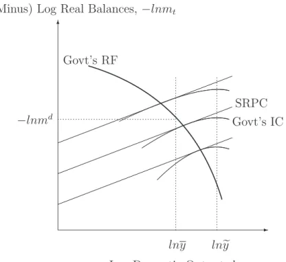
As α > n,υ(m) must be such thatυ0(m) +mυ00(m)<0, because, only in this case, will the marginal cost to inflating to be increasing in the discretionary rate of inflation. If, for example, υ(m) is logarithmic, the government’s reaction function will be vertical in (−lnm,lny) space, and a rational expectations equilibrium will only occur as a special case. Intuitively, this is because the governments set of indifference curves will be linear displacements of one another, which can be seen by holding utility constant, using the
constraint (26), and taking the derivative of (25) with respect to m. However, even if υ0(m) +mυ00(m) <0, y > ey is still a necessary condition for an equilibrium because otherwise the indifference curves will be negatively sloped in (−lnm,lny) space.15 These
two separate requirements are clear from the following representation of the optimization problem. -6 lny −lnmd lney Govt’s RF
Log Domestic Output, lnyt
(Minus) Log Real Balances, −lnmt
SRPC Govt’s IC
Figure 1: Government’s Optimization Problem
The short-run Phillips curve in figure one only allows for tangency points on the positively sloped portion of the government’s set of indifference curves, where the natural rate of output is below the socially optimal level. If the natural rate of output is above the social optimum the outcome of the game will not produce a feasible equilibrium. Second, the convex cost of holding nominal money (or rather of inflation) is also crucial for the equilibrium to be well defined. The special case in which the public and government reaction functions are vertical and coincide is similar to Beningo’s (2002) analysis of the 15It should be clear that asα > nthere are a family of positively sloped Phillips Curves in (−lnm,lny)
discretionary equilibrium. This case is also consistent with the ad-hoc Barro-Gordon model when the loss function is linear in inflation and quadratic in output.
4.2. Optimal Inflation
The final step in solving for the optimal rate of inflation is to equate equilibrium real balances with steady state real balances. In the steady state, real balances are stationary so mt = m and inflation is equal to the money growth rate such that µπ = 1, where
π denotes gross inflation. From the money demand function, this implies υ0(m) = (π−β)Cβ. Using (30), the discretionary rate of inflation, denotedπd, can be written in
the compact form,
πd/β = 1 +υ0¡md¢C
| {z }
inflation bias
(31)
Inflation is split between the Friedman rule level of inflation and a bias term representing the incentives that drive the government to inflate the economy. The Friedman level of inflation in this economy is πd =β and is the outcome when the government has access
to a commitment technology. The basic intuition for this result is that there is a wedge generated between the private and social marginal cost of holding money, and wheni >0, this generates an inefficiency. If there were no opportunity cost to holding money this inefficiency would disappear, but this requires that inflation equal the inverse of the real interest rate, which is given byβ. In turn, the bias term is split between consumption and real money balances. The consumption-real money balances split is important because, as I will argue, the consumption term, which appears from the use of micro-foundations, plays a role in overturning many of the results in the reduced-form literature, whilst the real balances part captures the essence of this approach.
To make progress I adopt the following functional form.
υ(m) = a²
²−1m
(²−1)/²
where a is the weight on real balances in utility and ² captures the elasticity of substi-tution between consumption and real money balances. The parameter ² also controls the convexity of the inflation cost and as ² → 1 the cost becomes linear such that it is
optimal for the government to raise the growth rate of money ever higher. To generate the discretionary equilibrium υ0(m) +mυ00(m) < 0 requires ² < 1.16 I now rewrite
inflation in terms of exogenous parameters only.
πd=β+aβ[(n−δ)/a(α−n)]1/(1−²) | {z } ≡(md)−1/² h (δ/φα)n/κα i [(1−n)/g∗]n−1 | {z } ≡C (32)
This makes clear that the equilibrium rate of inflation is a potentially complicated function of the degree of openness. There are three basic mechanisms through which openness affects inflation. The first term in square brackets represents the effect of changes in real money balances on utility, the second represents leisure and the final term the effect through trade-weighted export demand and the terms of trade.
4.2.1. Export Demand
An important preliminary result relates to the impact of export demand on inflation. It is clear that higher export demand leads to a higher rate of inflation, for a given degree of openness. The intuition for this result is straightforward because export demand only enters equation (32) through it’s impact on the terms of trade. Using the solution for the exchange rate and the natural rate of output, export demand can be shown to have a positive relationship with the terms of trade.
ρ= (1−n) (δ/φα)1/κα/g∗
whereρis the inverse terms of trade.17 When export demand rises, the terms of trade are
improved, and a one unit increase in output produces a bigger increase in consumption and a larger increase in utility. The temptation to inflate is greater and this increases inflation. This result can only be obtained once agents’ welfare is used to make policy decisions. Reduced-form approaches, such as Romer (1993), have not emphasized the significance of export demand on inflation. In the context of rising global inflation the analysis therefore presents a simple explanation of why inflation may rise in countries which exports commodities that are in high demand. Because export demand is exogenous from the
16This is also the empirically more reasonable case.
17Notice that a change in export demand has a larger effect on the terms of trade the more open the
viewpoint of the government this result also undermines the argument that it is possible to reduce any upward bias in inflation via institutional arrangements. Once there is an exogenous increase in export demand, any inflation already present in the economy will be exacerbated.
4.2.2. Openness
The major point I address is whether inflation has an inverse relationship with openness. However, inspecting (32) it is clear that inflation is related to inflation through all three channels stressed above. The reason is that it is not simply the Phillips curve that alters as openness changes. Previously it was shown that the optimal level of output changes with openness, and this is associated with the government’s set of indifference curves. A preliminary comment is that the relationship between openness and equilibrium real balances, which is associated with the Phillips curve, is unambiguous. Taking the derivative of (30) with respect to n,
∂md
∂n
1
md =²(α−δ)/(²−1)(α−n)(n−δ) (33)
The structural parameters of the economy are such that α > δ, n > δ, and ² < 1, and so (33) is negative. Relating this result back to inflation, recall from (31), that holding consumption constant,∂πd/∂md<0.18 Given this relationship, the effect of openness via
real balances is negative; a more open economy has a lower equilibrium rate of inflation. Thus the effect from real balances and the relationship between openness and inflation is similar to that in previous studies because surprise monetary expansions are more costly the more open the economy.
To fully describe the reaction of inflation it is necessary to consider how steady state con-sumption reacts to changes in openness. Taking the two parts of concon-sumption separately, see again (32), (δ/φα)n/κα is decreasing in n because δ/φα <1, and this counteracts the cost of lower real balances. The second term, [(1−n)/g∗]n−1, increases or decreases
with openness depending on level of export demand, g∗. We already know that inflation
is increasing in export demand because improvements in the terms of trade provide an 18Note also thatmdis independent ofg∗but thatπdis not because steady state consumption contains an interaction between openness and export demand.
incentive to inflate the economy. However, now it is clear that export demand influences the relationship between openness and inflation. Differentiating (32) with respect to n
results in the following expression.
∂πd
∂n
1
πd−β = 1 + [(α−δ)/Γ (1−²)] + [(1/κα) ln (δ/φα)] + ln [(1−n)/g
∗] (34)
where Γ ≡ (n−δ) (α−n) > 0. It is now possible to see how export demand affects the openness-inflation relationship and to identify the influence of openness on inflation through the three mechanisms which correspond to the three terms in square brackets in equation (34).19 It is again worth noting that the leisure effect, by itself, suggests
openness and inflation have a positive relationship and the real money balance effect suggests there is the standard negative relationship. Taking these two together, however, inflation has an unambiguously negative relation with openness.
Now consider the export demand channel. Recall that n is constrained from below by the monopoly distortion, δ, for the reasons discussed above. When the economy is very closed, (1−n) is near zero and this restriction becomes less important. In this case, the trade-weighted export demand term becomes more and more negative, giveng∗ >(1−n),
which must surely hold for high levels ofn. If (1−n)/g∗is sufficiently small, for example,
when n is near one and export demand is high, this term dominates the right-hand side of equation (34). In this case, inflation has a positive relation with openness. However, it is also clear that there is a limit to this effect. For a given level of export demand, as
n falls, the export demand term rises and may turn positive. A secondary role is played by the real money balances channel because the first term in square brackets is rising in openness for low values of n. Thus it is possible to identify a non-monotonic relationship between openness and inflation which, in this case, works through a tension between the impact of real balances and trade-weighted export demand on utility. If we think of g∗
as varying across time, which it surely must do, then this suggests a very tenuous link between openness and inflation in the data.
Initially, this result may appear surprising, but there is also a natural link with the existing theoretical literature. In analyzing the welfare implications of interdependence
and monetary policy Corsetti and Pesenti (2001) comment that domestic market failures, i.e. monopoly distortions, need not give rise to an inflation bias when looking at optimal policy because any bias in inflation depends on the relation of openness to other variables. This result essentially derives from the possibility of a beggar-thyself effect of monetary policy when an economy is relatively small via the terms of trade and disutility of leisure. That the analysis in Corsetti and Pesenti (2001) stops short of looking at optimal policy, instead focusing on the role of exogenous changes in the money supply, is less important. The analysis presented there and the three channels identified here both only arise when the representative agents utility function is used as the metric for policy decisions. 5. Conclusion
This paper develops a general equilibrium model of a small open economy to analyze the optimal rate of inflation under discretion. The paper makes two main contributions. First, it is one a few papers that analyzes discretionary monetary policy using a dynamic general equilibrium framework in an open economy. Second, it provides a strong case for the argument that the openness-inflation relationship is dependent on the structure of the economy. To repeat the basic argument. The standard mechanism suggests that inflation depends on openness because surprise monetary expansions affect the terms of trade. The more open the economy, the stronger this effect, and the more costly it is to inflate. Here, however, export demand also affects the terms of trade. This implies that inflation is dependent on export demand and the impact changes in export demand have on inflation depend on the degree of openness. The result is that the openness-inflation relationship depends on the level of export demand. If export demand is high this distorts the terms of trade to such an extent that inflation may rise with openness.
References
Albanesi, Stephania, Lawrence Christiano, and Varadarajan V. Chari (2003). Expecta-tions, Traps and Monetary Policy, Review of Economic Studies70, 715-741.
Arseneau, David, M. (2004). Expectations Traps in a New Keynesian Open Economy Model, Federal Reserve Board of Governors Finance and Economics Discussion Series 45. Armenter, Roc, and Martin Bodenstein (2005). Does the Time Consistency Problem Make Flexible Exchange Rates Look Worse than You Think?, mimeo, Federal Reserve Bank of New York.
Barro, Robert, J., and David B. Gordon (1983). A Positive Theory of Monetary Policy in a Natural Rate Model, Journal of Political Economy 91, 589-610.
Benigno, Pierpaolo (2002). A Simple Approach to International Monetary Policy Coor-dination, Journal of International Economics 57, 177-196.
Benigno, Gianluca, and Pierpaolo Benigno (2003). Price Stability in Open Economies, Review of Economic Studies 70, 743-764.
Clarida, Richard, Jordi Gali, and Mark Gertler (1999). The Science of Monetary Policy: A New Keynesian Perspective, Journal of Economic Literature 37, 1661-1707. Clarida, Richard, Jordi Gali, and Mark Gertler (2002). A Simple Framework for Inter-national Monetary Policy Analysis,Journal of Monetary Economics 49, 879-904. Corsetti, Giancarlo, and Paolo Pesenti (2001). Welfare and Macroeconomic Interdepen-dence, Quarterly Journal of Economics116, 421-446.
Danthine, Jean-Pierre, and John B. Donaldson (1986). Inflation and Asset Prices in an Exchange Economy, Econometrica 54, 585-606.
Ireland, Peter (1997). Sustainable Monetary Policies,Journal of Economic Dynamics and Control 22, 87-108.
King, Robert, and Alexander L. Wolman (2004). Monetary Discretion, Pricing Comple-mentarity and Dynamic Multiple Equilibria, Quarterly Journal of Economics 119, 1513-1553.
Lane, Philip (1997). Inflation in Open Economies, Journal of International Eco-nomics42, 327-347.
Nicolini, Juan-Pablo (1998). More on the Time Consistency Problem of Monetary Policy, Journal of Monetary Economics 41, 333-350.
Neiss, Katherine (1999). Discretionary Inflation in a General Equilibrium Model, Jour-nal of Money, Credit, and Banking 31, 357-372.
Obstfeld, Maurice, and Kenneth Rogoff (1983). Speculative Hyperinflations in Maximiz-ing Models: Can We Rule Them Out?, Journal of Political Economy 91, 675-687. Pappa, Evi (2004). Do the ECB and the Fed really need to Cooperate? Optimal Mone-tary Policy in a Two-Country World, Journal of Monetary Economics 53, 753-779. Persson, Mats, Thorsten Persson, Lars Svensson (2006). Time Consistency of Fiscal and Monetary Policy: A Solution, Econometrica 74, 193-212.
Rogoff, Kenneth (1985). Can International Monetary Co-operation be Counterproduc-tive?, Journal of International Economics 18, 199-217.
Romer, David (1993). Openness and Inflation: Theory and Evidence, Quarterly Jour-nal of Economics 108, 870-903.
Svensson, Lars (1985). Money and Asset Prices in a Cash-in-Advance Economy,Journal of Political Economy 93, 919-944.
Woodford, Michael (2003). Interest and Prices: Foundations of a Theory of Monetary Policy, Princeton NJ: Princeton University Press.