Alessandro Gavazza
, Simon Mongey, and Giovanni L.
Violante
Aggregate recruiting intensity
Article (Accepted version)
(Refereed)
Original citation: Gavazza, Alessandro and Mongey, Simon and Violante, Giovanni L (2017) Aggregate recruiting intensity.American Economic Review. ISSN 0002-8282
© 2017 American Economic Association
This version available at: http://eprints.lse.ac.uk/85652/
Available in LSE Research Online: November 2017
LSE has developed LSE Research Online so that users may access research output of the School. Copyright © and Moral Rights for the papers on this site are retained by the individual authors and/or other copyright owners. Users may download and/or print one copy of any article(s) in LSE Research Online to facilitate their private study or for non-commercial research. You may not engage in further distribution of the material or use it for any profit-making activities or any commercial gain. You may freely distribute the URL (http://eprints.lse.ac.uk) of the LSE Research Online website.
This document is the author’s final accepted version of the journal article. There may be differences between this version and the published version. You are advised to consult the publisher’s version if you wish to cite from it.
Aggregate Recruiting Intensity
∗
Alessandro Gavazza
, Simon Mongey
‡ §, and Giovanni L. Violante
¶August 22, 2017
Abstract
We develop an equilibrium model of firm dynamics with random search in the labor market where hiring firms exert recruiting effort by spending resources to fill vacancies faster. Con-sistent with microevidence, fast-growing firms invest more in recruiting activities and achieve higher job-filling rates. These hiring decisions of firms aggregate into an index of economy-wide recruiting intensity. We study how aggregate shocks transmit to recruiting intensity, and whether this channel can account for the dynamics of aggregate matching efficiency during the Great Recession. Productivity and financial shocks lead to sizable pro-cyclical fluctuations in matching efficiency through recruiting effort. Quantitatively, the main mechanism is that firms attain their employment targets by adjusting their recruiting effort in response to movements in labor market slackness.
Keywords: Aggregate Matching Efficiency, Firm Dynamics, Macroeconomic Shocks, Recruiting Intensity, Unemployment, Vacancies.
∗We thank Steve Davis, Jason Faberman, Mark Gertler, Bob Hall, Leo Kaas, Ricardo Lagos, and Giuseppe
Moscarini for helpful suggestions at various stages of this project, and our discussants Russell Cooper, Kyle Harkenoff, William Hawkins, Jeremy Lise, and Nicolas Petrosky-Nadeau for many useful comments. The views expressed herein are those of the authors and not necessarily those of the Federal Reserve Bank of Minneapolis or the Federal Reserve System.
‡London School of Economics and CEPR §Federal Reserve Bank of Minneapolis
1
Introduction
A large literature documents cyclical changes in the rate at which the US macroeconomy matches job seekers and employers with vacant positions. Aggregate matching efficiency, mea-sured as the residual of an aggregate matching function that generates hires from inputs of job seekers and vacancies, epitomizes this crucial role of the labor market. In fact, matching effi-ciency is a key determinant, over and above market tightness, of the aggregate job-finding rate, i.e. the speed at which idle workers are hired. Swings in the job-finding rate account for the bulk of unemployment fluctuations (Shimer,2012). Identifying the deep determinants of aggregate matching efficiency is therefore necessary to fully understand labor market dynamics.
The Great Recession represents a particularly stark episode of deterioration in aggregate matching efficiency. Our reading of the data, displayed in Figure 1, is that this decline con-tributed to a depressed vacancy yield, to a collapse in the job-finding rate, and to persistently higher unemployment following the crisis.
A number of explanations have been offered for the decline in aggregate matching efficiency during the recession, virtually all of which have emphasized the worker side.1 A shift in the composition of the pool of job seekers toward the long-term unemployed, by itself, goes a long way toward explaining the drop (Hall and Schulhofer-Wohl, 2015); however, as documented by Mukoyama, Patterson, and ¸Sahin (2014), workers’ job search effort is countercyclical and tends to compensate for compositional changes. Hornstein and Kudlyak (2016) include both margins in their rich measurement exercise and conclude that they offset each other almost exactly, leaving the entire drop in match efficiency from unadjusted data to be explained. A rise in occupational mismatch shows more promise, but it can account for at most one-third of the drop and for very little of its persistence (¸Sahin, Song, Topa, and Violante,2014).
The alternative view we set forth in this paper is that fluctuations in the effort with which firms try to fill their open positions affect aggregate matching efficiency. When aggregated over firms, we call this factor aggregate recruiting intensity. Our goal is to investigate whether this factor is an important source of the dynamics of aggregate matching efficiency, and to study the economic forces that shape how it responds to macroeconomic shocks.
1A notable exception is the model inSedláˇcek(2014) that generates endogenous fluctuations in match efficiency
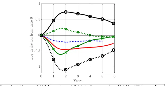
Figure 1: Labor market dynamics during the Great Recession (2008:01 - 2014:01) 0 1 2 3 4 5 6 Years -1 -0.5 0 0.5 1 L o g d ev ia ti o n fr o m d a te 0
Vacancies Vacancy yield Unemployment Jobfinding rate Agg. Matching Efficiency Entry
Notes:(i)VacanciesVtand hiresHt(used to compute vacancy yieldHt/Vt) taken from monthly Job Openings and Labor Turnover Survey
(JOLTS) data. Hires exclude recalls. (ii)UnemploymentUtis from the Bureau of Labor Statistics (BLS) and excludes workers on temporary
layoffs.(iii)The job-finding rate isHt/Ut.(iv)Aggregate matching efficiency is equal toHt/
Vα
tU1t−α
withα=0.5.(v)These first five series are measured from January 2001 to January 2014, expressed in logs and then HP-filtered. We plot level differences of these series from January 2008. (vi)(Firm) entry is taken from the Census Bureau’s Business Dynamics Statistics and computed annually as the number of firms aged less than or equal to one year at the time of survey and is available from 1977 to 2007. To this we fit and remove a linear trend. We plot log differences of this series from 2007.
Our main motivation is the empirical analysis of recruiting intensity at the micro level in
Davis, Faberman, and Haltiwanger(2013) (henceforthDFH)—the first paper to rigorously use JOLTS data to examine which factors are correlated with vacancy yields at the establishment level. The robust finding ofDFHis that establishments with a larger hiring rate (total hires per employment) fill their vacancies at a faster rate.2
One would therefore expect that, if an aggregate negative shock depresses firm growth rates, aggregate recruiting intensity—and, thus, aggregate match efficiency—declines since hiring firms use lower recruiting effort to fill their posted vacancies. We call this transmission chan-nel, whereby the macro shock affects the growth rate distribution of hiring firms, thecomposition
effect. Macro shocks also induce movements in equilibrium labor market tightness. When a
neg-ative shock hits the economy, job seekers become more abundant relneg-ative to vacancies, so firms
2The numerous exercises inDFHshow that this finding is not in any way spurious. For example, by definition,
an establishment that luckily fills a large amount of its vacancies will have both a higher vacancy yield and a higher growth rate. The authors show that luck does not drive their main result.
meet workers more easily and can therefore exert less recruiting effort to reach a given hiring target. We call this second transmission channel the slackness effect, in reference to aggregate labor market conditions.
Both mechanisms seem potentially relevant in the context of the Great Recession. As evident from Figure 1, the data display a collapse in market tightness indicating the potential for a strong slackness effect. The figure also shows that the rate at which firms entered the economy fell dramatically in the aftermath of the recession. The dominant narrative is that the crisis was associated with a sharp reduction in borrowing capacity, and start-up creation as well as young firm growth are particularly sensitive to financial shocks (Chodorow-Reich,2014;Siemer,2014;
Davis and Haltiwanger,2015;Mehrotra and Sergeyev, 2015). Combining this observation with the fact that much of job creation (and an even larger share of gross hires) are generated by young firms (Haltiwanger, Jarmin, and Miranda,2010) paves the way for a sizable composition effect.
Our approach is to develop a model of firm dynamics in frictional labor markets that can guide us to inspect the transmission mechanism of two common macroeconomic impulses— productivity and financial shocks—on aggregate recruiting intensity. The model is consistent with the stylized facts that are salient to an investigation of the interaction between macro shocks and recruiting activities: (i) it matches the DFH finding that increases in hiring rates are realized chiefly through increases in vacancy yields rather than increases in vacancy rates; (ii) it allows for credit constraints that hinder the birth of start-ups and slow the expansion of young firms; and (iii) it is set in general equilibrium, since the recruiting behavior of hiring firms depends on labor market tightness, which fluctuates strongly in the data (Shimer,2005).
Our model is a version of the canonical Diamond-Mortensen-Pissarides random matching framework with decreasing returns in production and nonconvex hiring costs (Cooper, Haltiwanger, and Willis, 2007; Elsby and Michaels, 2013; Acemoglu and Hawkins,
2014). The model simultaneously features a realistic firm life cycle, consistent with its clas-sic competitive setting counterparts (Jovanovic,1982; Hopenhayn,1992), and a frictional labor market with slack on both demand and supply sides. We augment this environment in three dimensions.
First, we allow for endogenous entry and exit of firms. This is a key element for under-standing the effects of macroeconomic shocks on the growth rates of hiring firms, since it is
Figure 2: Breakdown of spending on recruiting activities. Source: Bersin and Associates (O’Leonard,2011) t t Tools 1% Employment branding services 2% Professional networking sites 3% Print / newspapers / billboards 4% University recruiting 5% Applicant tracking system 5% Travel 8% Contractors 8% Employee referrals 9% Other 12% Job boards 14% Agencies / third-party recruiters 29%
well documented that young firms account for a disproportionately large fraction of job cre-ation, grow faster than old firms, and are more sensitive to financial conditions.
Second, we introduce a recruiting intensity decision at the firm level: besides the number of open positions that they are willing to fill in each period, hiring firms choose the amount of re-sources that they devote to recruitment activities. This endogenous recruiting intensity margin generates heterogeneous job-filling rates across firms. In turn, the sum of all individual firms’ recruitment efforts, weighted by their vacancy share, aggregates to the economy’s measured matching efficiency.
Third, we introduce financial frictions: incumbent firms cannot issue equity, and a constraint on borrowing restricts leverage to a multiple of collateralizable assets, as in
Evans and Jovanovic(1989).3
We parameterize our model to match a rich set of aggregate labor market statistics and firm-level cross-sectional moments. In choosing the recruiting cost function, we reverse-engineer a specification that allows the model to replicateDFH’s empirical relation between the job-filling rate and the hiring rate at the establishment level from the JOLTS microdata. Our
parameteri-3Other papers that consider various forms of financial constraints in frictional labor market models
in-clude Wasmer and Weil (2004), Petrosky-Nadeau and Wasmer (2013), Eckstein, Setty, and Weiss (2014), and Buera, Jaef, and Shin(2015), though none of these models displays endogenous fluctuations in match efficiency. An exception isMehrotra and Sergeyev(2013), where a financial shock has a differential impact across industries and induces sectoral mismatch between jobseekers and vacancies.
zation of this cost function is based on a novel source of data, a survey of recruitment cost and practices based on over 400 firms that are representative of the US economy. Figure 2 gives a breakdown of spending on all recruitment activities in which firms engage in order to attract workers and quickly fill their open positions, as reported by the survey. Our hiring cost function is meant to summarize all such components.
We find that both productivity and financial shocks—modeled as shifts in the collat-eral parameter—generate substantial procyclical fluctuations in aggregate recruiting intensity. However, the financial shock generates movements in firm entry, labor productivity, and bor-rowing that are consistent with those observed during the 2008 recession, whereas the pro-ductivity shock does not. The credit tightening accounts for approximately half of the drop in aggregate matching efficiency observed during the Great Recession through a decline in ag-gregate recruiting intensity. Notably, our model is consistent with a key cross-sectional fact documented by Moscarini and Postel-Vinay (2016): the vacancy yield of small establishments spiked up as the economy entered the downturn, whereas that of large establishments was much flatter. The reason is that the financial shock impedes the growth of a segment of very productive, already large, but relatively young, firms with much of their growth potential still unrealized. These firms drastically cut their hiring effort.
Our examination of the transmission mechanism indicates that the slackness effect is the dominant force: aggregate recruiting intensity falls mainly because the number of available job seekers per vacancy increases, allowing firms to attain their recruitment targets even by spending less on hiring costs. Surprisingly, the impact of the shock through the shift in the distribution of firm growth rates (and, in particular, the decline in firm entry and young-firm expansion) on aggregate recruiting intensity is quantitatively small. Two counteracting forces weaken this composition effect: (i) hiring firms are selected, and thus are relatively more pro-ductive than they are in steady state; and (ii) the rise in the abundance of job seekers, relative to open positions, allows productive firms—especially those that are financially unconstrained— to grow faster.
In an extension of the model, we augment the composition effect with a sectoral compo-nent by allowing permacompo-nent heterogeneity in recruiting technologies across industries. As
Davis, Faberman, and Haltiwanger (2013) document, construction and a few other sectors stand out in terms of their frictional characteristics by systematically displaying higher than
average vacancy filling rates. In addition, these are the industries that were hit hardest by the crisis. In agreement with Davis, Faberman, and Haltiwanger(2012b), our measurement exer-cise concludes that, in the context of the Great Recession, the shift in the composition of labor demand away from these high-yield sectors played a nontrivial role in the decline of aggregate recruiting intensity.
We argue that our taxonomy of slackness and composition channels is useful for three reasons. First, it offers a useful heuristic lens for thinking about the complex—sometimes offsetting—firm-level forces that determine the dynamics of aggregate hiring in response to a macroeconomic shock. Second, when the slackness effect is dominant, as we conclude, firms’ recruiting efforts are very responsive to the availability of job seekers relative to vacant posi-tions in the labor market. This, in turn, implies that any aggregate impulse that reduces labor market tightness will have an amplified impact on the aggregate job-finding rate through firms’ recruiting intensity decisions. Third, a strong slackness effect also implies that any policy inter-vention directed at raising unemployed workers’ search effort with the aim of accelerating their reentry into the employment ranks will, by lowering aggregate tightness, reduce firms’ recruit-ing effort, thus mitigatrecruit-ing the original intent of the policy. By the same logic, the endogenous response of recruiting effort to labor market tightness reinforces the direct impact of subsidies targeted to hiring firms.
To the best of our knowledge, only two other papers have developed models of recruiting intensity. Leduc and Liu(2017) extend a standard Diamond-Mortensen-Pissarides model to one in which a representative firm chooses search intensity per vacancy. Without firm heterogene-ity, they are unable to speak to the cross-sectional empirical evidence that recruiting intensity is tightly linked to firm growth rates, a key observation that we use to discipline our frame-work and assess the magnitude of the composition effect. Kaas and Kircher (2015) is the only other paper that focuses on heterogeneous job-filling rates across firms. In their directed search environment, different firms post distinct wages that attract job seekers at differential rates, whereas we study how firms’ costly recruiting activities determine differential job-filling rates. One would expect both factors to be important determinants of the ability of firms to grow rapidly. For example, from Austrian data, Kettemann, Mueller, and Zweimuller(2016) docu-ment that job-filling rates are higher at high-paying firms. However, after controlling for the firm component of wages, they remain increasing in firms’ growth rates, implying that wages
are not the whole story: employers use other instruments besides wages to hire quickly.
Moreover, while they (andLeduc and Liu, 2017) study aggregate productivity shocks—as we do as well—we further analyze financial shocks, a more natural choice if one’s attention is on the Great Recession. Finally, while aggregate recruiting intensity drops after a negative aggregate shock in both our model and theirs, the reasons for the drop fundamentally differ.
Kaas and Kircher (2015) argue that the drop depends on recruiting intensity being a concave function of firms’ hiring policies, whose dispersion across firms increases after a negative shock. Our decomposition of the transmission mechanism linking macroeconomic shocks and aggre-gate recruiting intensity allows us to infer that the main source of the drop is the increase in the number of available job seekers per vacancy, which allows firms to scale back their recruiting effort.
The rest of the paper is organized as follows. Section2 formalizes the nexus between firm-level recruiting intensity and aggregate match efficiency. Section3outlines the model economy and the stationary equilibrium. Section4describes the parameterization of the model and high-lights some cross-sectional features of the economy. Section5describes the dynamic response of the economy to macroeconomic shocks, explains the transmission mechanism, and outlines the main results of the paper. Section6examines the robustness of our main findings. Section7 concludes.
2
Recruiting Intensity and Aggregate Matching Efficiency
We briefly describe how we can aggregate hiring decisions at the firm level into an economy-wide matching function with an efficiency factor that has the interpretation of average recruit-ing intensity. This derivation follows DFH. For much of the paper, we abstract from quits and search on the job, and thus in our baseline model there is no role for replacement hiring: gross hires always equal the net growth of expanding firms. We discuss the implications of this as-sumption in Section6.
At date t, any given hiring firm i chooses vit, the number of open positions ready to be staffed and costly to create, as well as eit, an indicator of recruiting intensity. Letv∗it =eitvitbe
the number ofeffectivevacancies in firmi. Integrating over all firms, we obtain
Vt∗ =
ˆ
eitvitdi, (1)
the aggregate number of effective vacancies. Under our maintained assumption of a constant returns to scale Cobb-Douglas matching function, aggregate hires equal
Ht = (Vt∗)αUt1−α =ΦtVtαUt1−α, withΦt = Vt∗ Vt α = ˆ eit vit Vt di α , (2)
which corresponds to DFH’s generalized matching function. Therefore, measured aggregate matching efficiency Φt is an average of firm-level recruiting intensity weighted by individual vacancy shares, raised to the power of α, the economy-wide elasticity of hires to vacancies.
Finally, consistency requires that each firmifaces hiring frictions, implying that
hit =q(θ∗t)eitvit, (3)
where θt∗ = Vt∗/Ut is effective market tightness.4 Thus, q(θt∗) = Ht/Vt∗ = (θ∗t)
α−1 is the aggregate job-filling rate per effective vacancy, constant across all firms at datet.
3
Model
Our starting point is an equilibrium random-matching model of the labor market in which firms are heterogeneous in productivity and size, and the hiring process occurs through an ag-gregate matching function. As discussed in the introduction, we augment this model in three dimensions—all of which are essential to developing a framework that can address our ques-tion. First, our framework features endogenous firm entry and exit. Second, beyond the num-ber of positions to open (vacancies), hiring firms optimally choose their recruiting intensity: by spending more on recruitment resources, they can increase the rate at which they meet job seekers. Third, once in existence, firms face financial constraints.
In what follows, we present the economic environment in detail, outline the model timing,
4Throughout, we are faithful to the notation in this literature and denotemeasuredlabor market tightnessVt/Ut
and then describe the firm, bank, and household problems. Finally, we define a stationary equilibrium for the aggregate economy. Since our experiments will consist of perfect foresight transition dynamics, we do not make reference to aggregate state variables in agents’ problems. We use a recursive formulation throughout.
3.1
Environment
Time is discrete and the horizon is infinite. Three types of agents populate the economy: firms, banks, and households.
Firms. There is an exogenous measureλ0of potential entrants each period, and an endogenous measureλof incumbent firms. Firms are heterogeneous in their productivityz ∈ Z, stochastic and i.i.d. across all firms, and operate a decreasing returns to scale (DRS) production technology y(z,n′,k) that uses inputs of laborn′ ∈ N and capital k ∈ K. The output of production is a homogeneous final good, whose competitive price is the numeraire of the economy.
All potential entrants receive an initial equity injectiona0from households. Next, they draw a value of z from the initial distribution Γ0(z) and, conditional on this draw, decide whether to enter and become an incumbent by paying the setup cost χ0. Those that do not enter return the initial equity to the households.5 This is the only time when firms can obtain funds directly from households. Throughout the rest of their life cycle they must rely on debt issuance.
Incumbents can exit exogenously or endogenously. With probabilityζ, a destruction shock
hits an incumbent firm, forcing it to exit. Surviving firms observe their new value of z, drawn from the conditional distributionΓ(dz′,z), and choose whether to exit or continue production. Under either exogenous or endogenous exit, the firm pays out its positive net worthato house-holds. Those incumbents that decide to stay in the industry pay a per-period operating cost χ
and then choose labor and capital inputs.
The labor decision involves either firing some existing employees or hiring new workers. Firing is frictionless, but hiring is not: a hiring firm chooses both vacancies vand recruitment effortewith associated hiring costC(e,v,n), which also depends on initial employment. Given (e,v), the individual hiring function(3)determines current period employmentn′used in
pro-5Without loss of generality, we could have assumed that a fraction of the initial equity is sunk to develop the
duction. To simplify wage setting, we assume that firms’ owners make take-it-or-leave-it offers to workers, so the wage rate equalsω, the individual flow value from nonemployment.
Firms face two financial constraints. First, the capital decision involves borrowing capital from financial intermediaries (banks) in intraperiod loans. Because of imperfect contractual enforcement frictions, firms can appropriate a fraction 1/ϕ of the capital received by banks,
with ϕ > 1. To preempt this behavior, a firm renting k units of capital is required to deposit
k/ϕ units of their net worth with the bank. This guarantees that, ex post, the firm does not
have an incentive to abscond with the capital. Thus, a firm with current net worth a faces a collateral constraint k ≤ ϕa. This model of financial frictions is based onEvans and Jovanovic (1989). Second, as mentioned above, we assume that firms may only issue equity upon entry: an incumbent must keep nonnegative dividends.
The model requires both constraints. Without the equity (nonnegative dividend) constraint, firms can arbitrarily obtain funds from households. The collateral constraint will still impose a maximum ratio ofktoa, butacan increase freely through raised equity(d<0), sokis in effect
unconstrained. Without the collateral constraint, firms can arbitrarily increase k through debt while keeping dividends nonnegative. In both cases, the only limit is determined by the exit option (i.e., a negative continuation value).
Banks. The banking sector is perfectly competitive. Banks receive household deposits, freely transform them into capital, and rent it to firms. The one-period contract with households pays a risk-free interest rate of r. Capital depreciates at rate δ in production, and so the price of
capital charged by banks to firms is(r+δ).
Households. We envision a representative household with ¯Lfamily members,U of which are unemployed. The household is risk-neutral with discount factor β ∈ (0, 1). It trades shares
M of a mutual fund comprising all firms in the economy and makes bank depositsT. It earns interest on deposits, the total wage payments that firms make to employed family members, and Ddividends per share held in the mutual fund. Moreover, unemployed workers produce
ωunits of the final good at home. Household consumption is denoted byC.
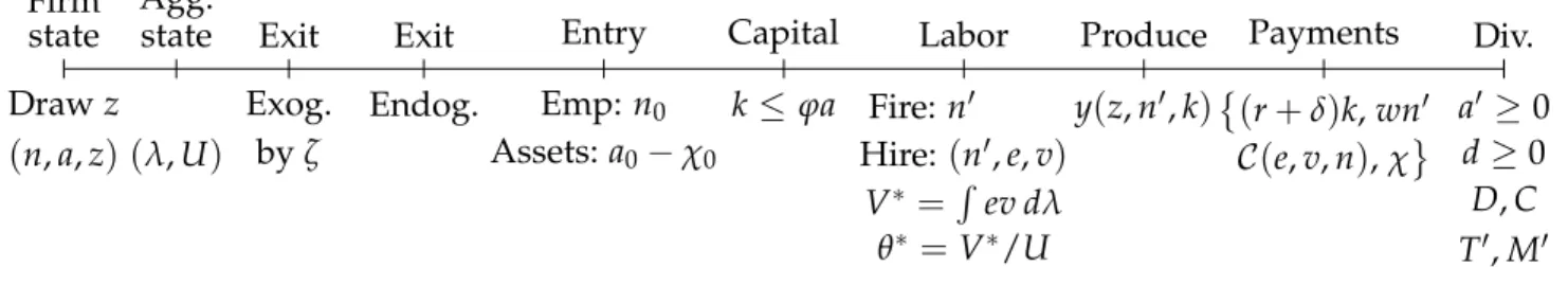
Before describing the firm’s problem in detail, we outline the precise timing of the model, summarized in Figure 3. Within a period, the events unfold as follows: (i) realization of the productivity shocks for incumbent firms; (ii) endogenous and exogenous exit of incumbents;
Drawz (n,a,z) Firm state Exog. byζ Exit Endog. Exit Emp: n0 Assets:a0−χ0 Entry k ≤ ϕa Capital Fire:n′ Hire:(n′,e,v) V∗ =´ ev dλ Labor θ∗ =V∗/U y(z,n′,k) Produce (r+δ)k,wn′ C(e,v,n),χ Payments a′ ≥0 d≥0 D,C Div. T′,M′ (λ,U) Agg. state
Figure 3: Timeline of the model
(iii) realization of initial productivity and entry decision of potential entrants; (iv) borrowing decisions by incumbents; (v) hiring/firing decisions and labor market matching; (vi) produc-tion and revenues from sales; (vii) payment of wage bill, costs of capital, hiring, and operaproduc-tion expenses, firm dividend payment/saving decisions, and household consumption/saving deci-sions.
To be consistent with our transition dynamics experiments in Section5, it is useful to note that we record aggregate state variables—the measures of incumbent firms λand
unemploy-mentU—at the beginning of the period, between stages (i) and (ii). Moreover, even though the labor market opens after firms exit or fire, workers who separate in the current period can only start searching next period.
3.2
Firm Problem
We first consider the entry and exit decisions, then analyze the problem of incumbent firms. Entry. A potential entrant who has drawnzfromΓ0(z)solves the following problem:
maxna0, Vi n0,a0−χ0,z o, (4)
where Vi is the value of an incumbent firm, a function of(n,a,z). The firm enters if the value to the risk-neutral shareholder of becoming an incumbent with one employee (n0 =1), initial net worth equal to the household equity injectiona0 minus the entry costχ0, and productivity
zexceeds the value of returninga0to the household. Leti(z) ∈ {0, 1}denote the entry decision rule, which depends only on the initial productivity draw, since all potential entrants share the same entry cost, initial employment and ex ante equity injection. AsViis increasing inz, there
is an endogenous productivity cutoff z∗ such that for allz ≥z∗, the firm chooses to enter. The measure of entrants is therefore
λe =λ0
ˆ
Z
i(z)dΓ0 =λ0h1−Γ0(z∗)i. (5)
Exit. Firms exit exogenously with probabilityζ. Conditional on survival the firm then chooses
to continue or exit. An exiting firm pays out its net worthato shareholders. The firm’s expected valueVbefore the destruction shock equals
V n,a,z =ζa+ (1−ζ)maxnVi n,a,z, ao. (6) We denote byx(n,a,z) ∈ {0, 1}the exit decision.
Hire or Fire. An incumbent firmi with employment, assets, and productivity equal to the triplet(n,a,z)chooses whether to hire or fire workers to solve
Vi n,a,z =max
n
Vh n,a,z,Vf n,a,zo. (7) The two value functions Vf and Vh associated with firing (f) and hiring (h) are described below.
The Firing Firm. A firm that has chosen to fire some of its workers (or to not adjust its work force) solves Vf n,a,z = max n′,k,d d+β ˆ Z V n′,a′,z′Γ(dz′,z) (8) s.t. n′ ≤ n, d+a′ = y n′,k,z+ (1+r)a−ωn′−(r+δ)k−χ, k ≤ ϕa, d ≥ 0.
Firms maximize shareholder value and, because of risk neutrality, useβas their discount factor.
net of the wage bill, rental and operating costs, and dividend payoutsd. The last two equations in (8) reiterate that firms face a collateral constraint on the maximum amount of capital they can rent and a nonnegativity constraint on dividends.
To help understand the budget constraint and preface how we take the model to the data, define firm debt by the identityb ≡ k−a, with the understanding thatb < 0 denotes savings.
Making this substitution reveals an alternative formulation of the model in which the firm owns its capital and faces a constraint on leverage. With state vector (n,k,b,z), the firm faces the following budget and collateral constraints:
d+k′−(1−δ)k | {z } Investment = y(n′,k,z)−ωn′−χ−rb | {z } Operating Profit + b′−b | {z } ∆Borrowing , b/k ≤ (ϕ−1)/ϕ.
This makes it clear that the firm can fund equity payouts and investment in capital through either operating profits or expanding borrowing/reducing saving.
The Hiring Firm. The hiring firm additionally chooses the number of vacancies to postv ∈R+ and recruitment effort e ∈ R+, understanding that, by a law of large numbers, its new hires n′−nequal the firm’s job-filling rateqeof each of its vacancies times the number of vacancies v created: n′−n = q(θ∗)ev.6 Note that the individual firm job-filling rate depends on the aggregate meeting rate q, which is determined in equilibrium and the firm takes as given, as well as on its recruiting efforte. The firm faces a variable cost functionC(e,v,n), increasing and convex ineandv.
A firm’s continuation value depends onn′, not on the mix of recruiting intensityeand vacant positions v that generates it. As a result, one can split the problem of the hiring firm into two stages. The first stage is the choice ofn′,k, andd. The second stage, givenn′, is the choice of the optimal combination of inputs(e,v). The latter reduces to a static cost minimization problem:
C∗ n,n′ =min
e,v C(e,v,n) (9)
s.t. e≥0, v≥0, n′−n=q(θ∗)ev,
yielding the lowest cost combination e(n,n′) and v(n,n′) that delivers h = n′−n hires to a firm of sizen, and the implied cost functionC∗(n,n′).
The remaining choices ofn′,k, anddrequire solving the dynamic problem Vh(n,a,z) = max n′,k,d d+β ˆ Z V(n′,a′,z′)Γ(dz′,z) (10) s.t. n′ > n, d+a′ = y(n′,k,z) + (1+r)a−ωn′−(r+δ)k−χ− C∗ n,n′, k ≤ ϕa, d ≥ 0.
The solution to this problem includes the decision rule n′(n,a,z). Using this function in the solution to (9), we obtain decision rules e(n,a,z) and v(n,a,z) for recruitment effort and va-cancies in terms of firm state variables.
Given the centrality of the hiring cost functionC(e,v,n) to our analysis, we now discuss its
specification. In what follows, we choose the functional form
C(e,v,n) = κ1 γ1e γ1+ κ2 γ2+1 v n γ2 v, (11)
with γ1 ≥ 1 and γ2 ≥ 0 being necessary conditions for the convexity of the maximization problem (9). This cost function implies that the average cost of a vacancy,C/v, has two separate components. The first is increasing and convex in recruiting intensity per vacancy e. The idea is that, for any given open position, the firm can choose to spend resources on recruitment activities (recall Figure 2) to make the position more visible or the firm more attractive as a potential employer, or to assess more candidates per unit of time, but all such activities are increasingly costly on a per-vacancy basis. The second component is increasing and convex in the vacancy rate and captures the fact that expanding productive capacity is costly in relative terms: for example, creating 10 new positions involves a more expensive reorganization of production in a firm with 10 employees than in a firm with 1,000 employees.
In AppendixAwe derive several results for the static hiring problem of the firm(9)under this cost function and derive the exact expression for C∗(n,n′) used in the dynamic problem
(10). We show that, by combining first-order conditions, we obtain the optimal choice fore: e n,n′ = κ2 κ1 γ1 γ1−1 γ 1 1+γ2 q(θ∗)− γ2 γ1+γ2 n′−n n γγ2 1+γ2 , (12)
and, hence, the firm-level job-filling rate f (n,n′) ≡ q(θ∗)e(n,n′), as well as the optimal va-cancy rate: v n = κ2 κ1 γ1 γ1−1 γ 1 1+γ2 q(θ∗)− γ1 γ1+γ2 n′−n n γγ1 1+γ2 . (13)
Equation (12) demonstrates that the model implies a log-linear relation between the job-filling rate and employment growth at the firm level, with elasticity γ2/(γ1+γ2). This is the key empirical finding of DFH, who estimate this elasticity to be 0.82. In fact, one could interpret our functional choice forCin equation(11)as a reverse-engineering strategy in order to obtain,
from first principles, the empirical cross-sectional relation between the establishment-level job-filling rate and the establishment-level hiring rate uncovered byDFH. Put differently, microdata sharply discipline the recruiting cost function of the model.7
Why does firm optimality imply that the job-filling rate increases with the growth rate with elasticityγ2/(γ1+γ2)? Recruiting intensityeand the vacancy rate(v/n)are substitutes in the production of a target employment growth rate (n′−n)/n(see the last equation in(9)). Thus,
a firm that wants to grow faster than another will optimally create more positions and, at the same time, spend more in recruiting effort. However, the stronger the convexity of C in the vacancy rate (γ2), relative to its degree of convexity in effort(γ1), the more an expanding firm finds it optimal to substitute away from vacancies into recruiting intensity to realize its target growth rate. In the special case whenγ2 =0, all the adjustment occurs through vacancies, and recruiting effort is irresponsive to the growth rate and to macroeconomic conditions, as in the canonical model ofPissarides(2000).
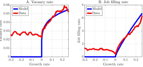
Figure 4 plots the cross-sectional relationship between the vacancy rate and employment growth (panel A) and the job-filling rate and employment growth (panel B) in the model and
7AppendixAalso shows that, once the optimal choice ofeis substituted into(11),C can be stated solely in
terms of the vacancy rate and becomes equivalent to one of the hiring cost functions thatKaas and Kircher(2015) use in their empirical analysis.
Figure 4: Cross-sectional relationships between monthly employment growth (n′−n)/n and the vacancy rate v/nand the job-filling rateeq. Data fromDFHonline supplemental materials.
-0.3 -0.2 -0.1 0 0.1 0.2 Growth rate 0 0.01 0.02 0.03 0.04 0.05 0.06 V a ca n cy ra te A. Vacancy rate Model Data -0.3 -0.2 -0.1 0 0.1 0.2 Growth rate 0 2 4 6 8 J o b fi ll in g ra te
B. Jobfilling rate
Model Data
in the DFHdata, with the elasticity of the job-filling rate to firm growthγ2/(γ1+γ2) =0.82.8 Since the individual hiring function is linear in vacancies, the elasticity of the vacancy rate to firm growth equalsγ1/(γ1+γ2) =0.18.
3.3
Household Problem
The representative household solvesW(T,M,D) = max
T′,M′,C>0
C+βW(T′,M′,D′) (14)
s.t.
C+QT¯ ′+PM′ = ωL¯ + (D+P)M+T,
where Tare bank deposits, Mare shares of the mutual fund composed of all firms in the econ-omy, andDare aggregate dividends per share.9 The household takes as given the price of bank deposits ¯Q, the share priceP, and the price of the final good, which we normalize to one. From the first-order conditions for deposits and share holdings, we obtain ¯Q= βand P= β(P+D)
which imply a time-invariant rate of return of r = β−1−1 on both deposits and shares. The
8In Figure4, the model implies zero hires for firms with negative growth rates, whereas in the data time
ag-gregation and replacement hires lead to positive vacancy rates and vacancy yields for shrinking firms as well. We return on this point in Section6.
9The initial equity injections into successful start-ups are treated as negative dividends, i.e. they are part ofD
household is therefore indifferent over portfolios.
Since firms make take-it-or-leave-it offers to workers (i.e., firms have all the bargaining power) and are competitive, they pay all their workers a wage equal to the individual’s flow value of nonemployment ω, which we interpret as output from home production. The total
amount of resources available to households for consumption and saving as a result of market and home production is thus simplyωL¯.10 Because of risk neutrality, the household is indiffer-ent over the timing of consumption.
3.4
Stationary Equilibrium and Aggregation
Let ΣN, ΣA, and ΣZ be the Borel sigma algebras over N and A, and Z. The state space for an incumbent firm is S = N×A×Z, and we denote with s one of its elements (n,a,z). Let
ΣS be the sigma algebra on the state space, with typical set S =N × A × Z, and (S,ΣS) be the corresponding measurable space. Denote with λ : ΣS → [0,∞) the stationary measure of incumbent firms at the beginning of the period, following the draw of firm-level productivity, before the exogenous exit shock.
To simplify the exposition of the equilibrium, it is convenient to use s ≡ (n,a,z) and s0 ≡
(n0,a0−χ0,z)as the argument for incumbents’ and entrants’ decision rules.
A stationary recursive competitive equilibrium is a collection of firms’ decision rules
{i(z),x(s),n′(s),e(s),v(s),a′(s),d(s),k(s)}, value functionsV,Vi,Vf,Vh , a measure of entrants λe, share price P and aggregate dividends D, wage ω, a distribution of firms λ, and
a value for effective labor market tightness θ∗ such that: (i) the decision rules solve the firm’s
problems (4)-(10), V,Vi,Vf,Vh are the associated value functions, and λe is the mass of entrants implied by (5); (ii) the market for shares clears atM =1 with share price
P = ˆ S V(s)dλ+λ0 ˆ Z i(z)Vi(s0)dΓ0
10If we let the wage be W, then total resources from market and home production equalW(L¯ −U) +ωU.
The term ωL¯ in the household budget constraint follows from the fact thatW = ω. This also explains why
and aggregate dividends D=ζ ˆ S adλ+ (1−ζ) ˆ S {[1−x(s)]d(s) +x(s)a}dλ−λ0 ˆ Z i(z)a0dΓ0;
(iii) the stationary distribution λis the fixed point of the recursion: λ(N × A × Z) = (1−ζ) ˆ S [1−x(s)]1{n′(s)∈N }1{a′(s)∈A}Γ(Z,z)dλ (15) +λ0 ˆ Z i(z)1{n′(s0)∈N }1{a′(s0)∈A}Γ(Z,z)dΓ0,
where the first term refers to existing incumbents and the second to new entrants; (iv) effective market tightnessθ∗ is determined by the balanced flow condition
¯
L−N(θ∗) = F(θ
∗)−λ
e(θ∗)n0
p(θ∗) , (16)
where p(θ∗)is the aggregate job-finding rate, N(θ∗)is aggregate employment N(θ∗) = (1−ζ) ˆ S [1−x(s)]n′(s)dλ+λ0 ˆ Z i(z)n′(s0)dΓ0, (17)
and F(θ∗)are aggregate separations
F(θ∗) = ζ ˆ S ndλ+ (1−ζ) ˆ S x(s)ndλ+ (1−ζ) ˆ S [1−x(s)] n−n′(s)−dλ, (18)
which include all employment losses from firms exiting exogenously and endogenously, plus all the workers fired by shrinking firms, which we have denoted by(n−n′(s))−.11 In equations
(16)-(18), the dependence of λe, N, and F on θ∗ comes through the decision rules and the
stationary distribution, even though, for notational ease, we have omitted θ∗ as their explicit
argument.
The left-hand side of (16) is the definition of unemployment—labor force minus employment—whereas the right-hand side is the steady state Beveridge curve, i.e., the law
11Entrant firms never fire, as they enter with the lowest value on the support forN,n
of motion for unemployment
U′ =U−p(θ∗)U+F(θ∗)−λe(θ∗)n0 (19)
evaluated in steady state. As in Elsby and Michaels (2013), the two sides of (16) are inde-pendent equations determining the same variable—unemployment—and combined they yield equilibrium market tightness θ∗.12 Note that equations (16) and (19) account for the fact that
every new firm enters withn0workers hired “outside” the frictional labor market (e.g., the firm founders).
Clearly, once θ∗ and λ are determined, so isU from either side of (16) and, therefore, V∗. Finally, we note that measured aggregate matching efficiency, in equilibrium, is Φ= (V∗/V)α, where measured and effective vacancies are respectively
V = (1−ζ) ˆ S [1−x(s)]v(s)dλ +λ0 ˆ Z i(z)v(s0)dΓ0, V∗ = (1−ζ) ˆ S [1−x(s)]e(s)v(s)dλ+λ0 ˆ Z i(z)e(s0)v(s0)dΓ0.
AppendixCprovides details on the computation of the decision rules and the stationary equi-librium.
4
Parameterization
We begin with the subset of parameters calibrated externally, then consider those estimated within the model. The main problem we face in parameterizing the model is that the theory does not distinguish between firms and establishments. Ideally we would only use data on firms, since financial constraints apply at the firm level. However JOLTS data is only available by establishment, as are other data sources we use in calibration. We are therefore forced to compromise: we use firm data whenever we have a choice—for example, when we use the
12Our computation showed that, typically, N(θ∗)is decreasing in its argument and the right-hand side of(16)
is always positive and decreasing. Thus, the crossing point of the left- and right-hand sides is unique, when it exists. However, an equilibrium may not exist. For example, for very low hiring costs,N(θ∗)may be greater than
¯
L. Conversely, for large enough operating or hiring costs, no firms will enter the economy. In this case, there is no equilibrium with market production (albeit there is always some home production in the economy).
Table 1: Externally set parameter values
Parameter Value Target Value
Discount factor (monthly) β 0.9967 Annual risk-free rate 0.04
Mass of potential entrants λ0 0.02 Measure of incumbents 1
Size of labor force L¯ 24.6 Average firm size (BDS) 23
Elasticity of matching function wrtVt α 0.5 JOLTS
Business Dynamics Statistics (BDS) data—and establishment data when we are limited. Data moments are averages over 2001-2007 unless otherwise specified.
4.1
Externally Calibrated
The model period is one month. We setβto replicate an annualized risk-free rate of 4 percent.
Since the measure of potential entrants λ0 scales λ—see equation (15)—we choose λ0 to nor-malize the total measure of incumbent firms to one. We then fix the size of the labor force ¯L so that, given a measure one of firms, and the model implied steady-state unemployment rate of 7 percent, the average firm size will be 23 (BDS).13 In line with empirical studies, we set α, the elasticity of aggregate hires to aggregate vacancies in the matching function, to 0.5. Table1 summarizes these parameter values.
4.2
Internally Calibrated
Table 2 lists the remaining 19 parameters of the model that are set by minimizing the dis-tance between an equal number of empirical moments and their equilibrium counterparts in the model.14 It also lists the targeted moments, their empirical values, and their simulated val-ues from the model. Even though every targeted moment is determined simultaneously by all parameters, in what follows we discuss each of them in relation to the parameter for which,
13The unemployment rate isu = L¯/N(θ∗)−1, and with a unit mass of firms the average firm size is simply
N(θ∗). Hence for an unemployment rate ofu=0.07, ¯Ldetermines average firm size.
14Specifically, the vector of parametersΨis chosen to minimize the minimum-distance-estimator criterion
func-tion
f(Ψ) = (mdata−mmodel(Ψ))′W(mdata−mmodel(Ψ))
where mdata and mmodel(Ψ) are the vectors of moments in the data and model, and W = diag 1/m2data
is a diagonal weighting matrix.
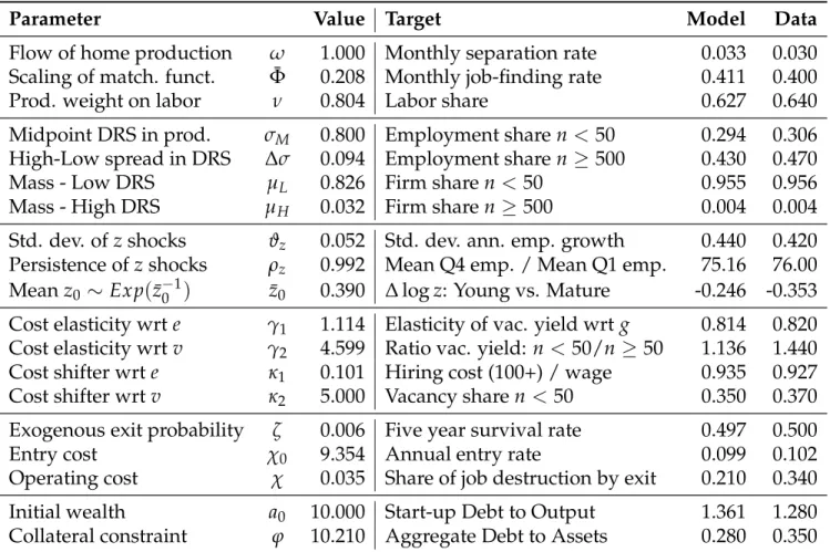
Table 2: Parameter values estimated internally
Parameter Value Target Model Data
Flow of home production ω 1.000 Monthly separation rate 0.033 0.030
Scaling of match. funct. Φ¯ 0.208 Monthly job-finding rate 0.411 0.400
Prod. weight on labor ν 0.804 Labor share 0.627 0.640
Midpoint DRS in prod. σM 0.800 Employment sharen<50 0.294 0.306
High-Low spread in DRS ∆σ 0.094 Employment sharen≥500 0.430 0.470
Mass - Low DRS µL 0.826 Firm sharen<50 0.955 0.956
Mass - High DRS µH 0.032 Firm sharen≥500 0.004 0.004
Std. dev. ofzshocks ϑz 0.052 Std. dev. ann. emp. growth 0.440 0.420
Persistence ofzshocks ρz 0.992 Mean Q4 emp. / Mean Q1 emp. 75.16 76.00
Meanz0∼Exp(z¯0−1) z¯0 0.390 ∆logz: Young vs. Mature -0.246 -0.353
Cost elasticity wrte γ1 1.114 Elasticity of vac. yield wrtg 0.814 0.820
Cost elasticity wrtv γ2 4.599 Ratio vac. yield: n<50/n ≥50 1.136 1.440
Cost shifter wrte κ1 0.101 Hiring cost (100+) / wage 0.935 0.927
Cost shifter wrtv κ2 5.000 Vacancy sharen <50 0.350 0.370
Exogenous exit probability ζ 0.006 Five year survival rate 0.497 0.500
Entry cost χ0 9.354 Annual entry rate 0.099 0.102
Operating cost χ 0.035 Share of job destruction by exit 0.210 0.340
Initial wealth a0 10.000 Start-up Debt to Output 1.361 1.280
Collateral constraint ϕ 10.210 Aggregate Debt to Assets 0.280 0.350
intuitively, that moment yields the most identification power.
We set the flow of home production of the unemployedω to replicate a monthly separation
rate of 0.03. We choose the shift parameter of the matching function (a normalization of the value of Φ in steady state) in order to replicate a monthly job-finding rate of 0.40. Together, these two moments yield a steady state unemployment rate of 0.07.
We assume a revenue function y(z,n′,k) = z(n′)νk1−νσ. We need not take a stand on whether zrepresents demand or productivity shocks, or whether σ < 1 is due to DRS in
pro-duction or downward-sloping demand.15 For simplicity, we will refer to the revenue function as if it were a production function: σrepresents the span of control andzis total factor produc-tivity.
15Given our class of frictions, the revenue function is sufficient. This would not be the case in alternative
en-vironments that endogenize components of revenue productivity, for example models with R&D—which affects productivity—or models with customer accumulation—which affects demand.
We introduce a small degree of permanent heterogeneity in the scale parameterσ.
Specifi-cally, we consider a three-point distribution with support{σL,σM,σH}—symmetric aboutσM—
leaving four unknown parameters: (i) the value of σM; (ii) the spread ∆σ ≡ (σH −σL); and
(iii)-(iv) the fractions of low and high DRS firmsµL,µH. This heterogeneity allows us to match
the skewed firm size distribution, with the parameters chosen to match the shares of total em-ployment and total firms due to firms of size 0-49 and 500+ (BDS). Permanent heterogeneity in productivity could also be used to match these facts, but heterogeneity in σ also generates
small old firms alongside young large firms, thus decoupling age and size, which tend to be too strongly correlated in standard firm dynamics models with mean reverting productivity.16 In other words, heterogeneity inσcaptures the appealing idea that there exist some very
produc-tive businesses that are small simply because the optimal scale of production for many goods or services is small. This idea will turn out to be important for interpreting the response of firms to a macroeconomic shock.
Firm productivity z follows an AR(1) process in logs: logz′ = logZ +ρzlogz+ε, with ε ∼ N(−ϑ2z/2,ϑz). We calibrate ρz and ϑz to match two measures of employment
disper-sion, one in growth and one in levels: the standard deviation of annual employment growth for continuing establishments in the US Census Bureau’s Longitudinal Business Database (Elsby and Michaels, 2013) and the ratio of the mean size of the fourth to first quartile of the firm distribution (Haltiwanger,2011).17
The initial productivity distribution for entrants Γ0 is exponential. The mean ¯z0 is chosen to match the revenue productivity gap between entrants and incumbents, specifically the differential between plants younger than age 1 and older than age 10 (Foster, Haltiwanger, and Syverson,2016).
We now turn to hiring costs. The cost function(11)has four parameters: the two elasticities (γ1,γ2)and the two cost shifters(κ1,κ2). From our discussion of equations (11) and (12), recall that the cross-sectional elasticity of the job-filling rate to employment growth, estimated to be 0.82 by DFH, is a function of the ratio of these two elasticities.18 The second moment used to
16SeeElsby and Michaels(2013) andKaas and Kircher(2015) for examples of the use of heterogeneity in
perma-nent productivity.
17In the numerical solution and simulation of the model,zremains a continuous state variable. 18We cannot mapγ
2/(γ1+γ2)directly into this value since inDFH, and in the model’s simulations for
con-sistency, the growth rate is the Davis-Haltiwanger growth rate normalized in[−2, 2]. In practice, as seen in Table
separately identify the two elasticities is the ratio of vacancy yields at small (n < 50) and large
(n ≥ 50) establishments (JOLTS). Intuitively, when γ2 = 0, recruiting effort is constant across firms and this ratio is one.
We use two targets to pin down the cost shift parameters. The first is the total hiring cost as a fraction of monthly wage per hire, a standard target for the single vacancy cost parameter that usually appears in vacancy posting models. We have a new source for this statistic. The con-sulting company Bersin and Associates runs a periodic survey of recruitment cost and practices based on over 400 firms—all with more than 100 employees. Once the firms are reweighted by industry and size, the sample is representative of this size segment of the US economy. They compute that, on average, annual spending on all recruiting activities (including internal staff compensation, university recruiting, agencies/third-party recruiters, professional networking sites, job boards, social media, contractors, employment branding services, employee refer-ral bonuses, pay-per-click media, travel to interview candidates, applicant tracking systems, print/media/billboards, and other tools/technologies) divided by the number of hires in 2011 was $3,479 (see Table 3 inO’Leonard 2011). Given average annual earnings of roughly $45,000 in 2011, in the model we target a ratio of average recruiting cost to average monthly wage (in firms with more than 100 employees) of 0.928. The second target is the vacancy share of small (n< 50) establishments from JOLTS:κ2determines the size of hiring costs for small firms and,
thus, the amount of vacancies they create.
The parametersχand ζ have large effects on firm exit. The operating cost χmostly affects
the exit rates of young firms; therefore, we target the five-year firm survival rate which is ap-proximately 50 percent (BDS). The parameter ζ contributes to the exit of large and old firms;
hence, we target the fraction of total job destruction due to exit of 34 percent (BDS).19 To pin down the setup costχ0, we target the annual firm entry rate of 10 percent (BDS).20
The remaining two parameters are the size of the initial equity injectiona0and the collateral relationship between the job-filling rate and thegross hires raterather than employment growth. In our model, the
gross hires rate and rate of employment growth of hiring firms coincide, although this would not be the case in a model with replacement hires. We discuss this in Section6.
19Unlike other moments used here from the BDS, job destruction by exit is only available by establishment exit,
not firm exit.
20When computing moments designed to be comparable to their counterparts in the BDS, we carefully
time-aggregate the model to an annual frequency. For example, the entry rate in the BDS is measured as the number of age zero firms in a given year divided by the total number of firms. Computing this statistic in the model requires aggregating monthly entry and exit over 12 months. See AppendixCfor details.
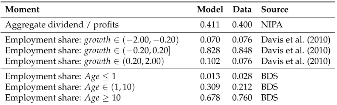
Table 3: Nontargeted moments
Moment Model Data Source
Aggregate dividend / profits 0.411 0.400 NIPA
Employment share: growth ∈ (−2.00,−0.20) 0.070 0.076 Davis et al. (2010)
Employment share: growth ∈ (−0.20, 0.20] 0.828 0.848 Davis et al. (2010) Employment share: growth ∈ (0.20, 2.00) 0.102 0.076 Davis et al. (2010)
Employment share: Age≤1 0.013 0.028 BDS
Employment share: Age∈ (1, 10) 0.309 0.212 BDS
Employment share: Age≥10 0.678 0.760 BDS
Notes:(i)NIPA data from Tables 2.1 and 5.1 for 2006, computed asDividends/(Corporate profits + (1/3)×Proprietor’s Income). (ii)Growth rate distribution statistics are computed from Table 2 ofDavis, Faberman, Haltiwanger, and Rucker(2010), which summarizes the distribution of employment by quarterly establishment growth rates in the Business Employment Dynamics (BED) data from 2001-2006. Growth rates are computed asgit= (nit+1−nit)/(0.5nit+0.5nit+1). We have removed entry and exit since we already match the entry rate in the calibration
so consider the distribution only over continuing establishments. Statistics from the model are also quarterly. (iii)BDS data are the average distribution of employment across firms from 2001-2007.
parameter ϕ. To inform their calibration, we target the debt-output ratio of start-up firms
com-puted from the Kauffman Survey (Robb and Robinson, 2014) and the aggregate debt to total assets ratio from the flow of funds accounts.21
4.3
Cross-Sectional Implications
We now explore the main cross-sectional implications of the calibrated model, at its steady state equilibrium.
Table 3 reports some empirical moments not targeted in the calibration and their model-generated counterparts. The fact that the ratio of dividend payments to profits in the model is close to its empirical value confirms that the collateral constraint is neither too tight nor too loose. The model can also replicate well the distribution of employment by establishment growth rate and firm age, neither of which was explicitly targeted.
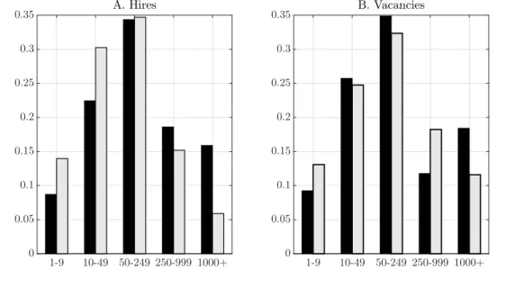
Figure5shows that the model is also able to satisfactorily replicate the observed distribution
21Robb and Robinson(2014) report $68,000 of average debt (credit cards, personal and business bank loans, and
credit lines) and $53,000 of average revenue for the 2004 cohort of start-ups in their first year; see their Table 5. From the flow of funds 2005, we computed total debt as the sum of securities and loans and total assets as the sum of all nonfinancial assets plus financial assets net of trade receivables, FDIs, and miscellaneous liabilities (Tables L.103 and L.104, Liabilities of Nonfinancial Corporate and Noncorporate Business), divided by the sum of corporate and noncorporate net worth (Tables B.103 and B.104, Balance Sheet of Nonfinancial Corporate and Noncorporate Business).
Figure 5: Hire and vacancy shares by size class. Model (black) and JOLTS data, 2002-2007 (grey). 1-9 10-49 50-249 250-999 1000+ 0 0.05 0.1 0.15 0.2 0.25 0.3 0.35 A. Hires 1-9 10-49 50-249 250-999 1000+ 0 0.05 0.1 0.15 0.2 0.25 0.3 0.35 B. Vacancies
of hires and vacancies by size class (JOLTS).
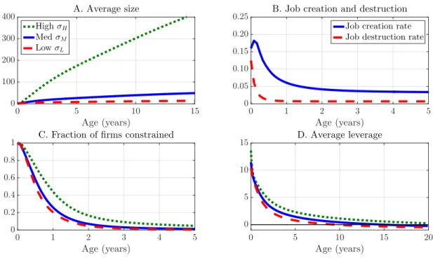
In Figure 6 we plot the average firm size, job creation and destruction rates, fraction of constrained firms, and leverage (debt/saving over net worth,b/a) for firms from birth through to maturity. Panel A shows thatσH firms, those with closer to constant returns in production,
account for the upper tail in the size and growth rate distributions. On average, though, firm size grows by much less over the life cycle, since these “gazelles”—as they are often referred to in the literature—are only a small fraction of the total (µH =0.032). This lines up well with the
data: average firm size grows by a factor of 3.0 between ages 1-5 and 20-25 in the model and 3.1 in the data (BDS). Convex recruiting costs and collateral constraints slow down growth: most firms reach their optimal size around age 10, whereasσH firms keep growing for much longer.
Panel B plots job creation and destruction rates by age and is a stark representation of the “up-and-out” dynamics of young firms documented in the literature (Haltiwanger,2012). Panel C depicts the fraction of constrained firms (defined as those withk= ϕaandd=0) over the life cycle. In the model, financial constraints bind only for the first few years of a firm’s life, when net worth is insufficient to fund the optimal level of capital. Panel D illustrates that leverage declines with age, and after age 10 the median firm is saving (i.e., b < 0). Much like in the
classical household “income fluctuation problem,” in our model firms have a precautionary saving motive because of the simultaneous presence of three elements: (i) a concave payoff function because of DRS, (ii) stochastic productivity, and (iii) the collateral constraint.
Figure 6: Average life cycle of firms in the model 0 1 2 3 4 5 Age (years) 0 0.05 0.10 0.15 0.20
0.25 B. Job creation and destruction
Job creation rate Job destruction rate
0 5 10 15 Age (years) 0 100 200 300 400 A. Average size HighσH MedσM LowσL 0 1 2 3 4 5 Age (years) 0 0.2 0.4 0.6 0.8 1 C. Fraction offirms constrained 0 5 10 15 20 Age (years) 0 5 10 15 D. Average leverage
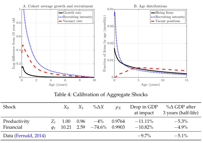
Panel A of Figure7shows that recruiting intensity and the vacancy rate are sharply decreas-ing with age. These features arise because our cost function implies that both optimal hirdecreas-ing effort and the vacancy rate are increasing in the growth rate, and young firms are those with the highest desired growth rates. Moreover, the stronger convexity of C in the vacancy rate (γ2), relative to its degree of convexity in effort(γ1)implies that a rapidly expanding firm prefers to increase its recruiting intensity relatively more than vacancies to realize its target growth rate. Thus, young firms find it optimal to recruit very aggressively for the new positions that they open. As firms age, growth rates fall and this force weakens.
Panel B plots the fraction of total recruiting effort, vacancies, and hiring firms by age. It shows that, relative to the steady state age distribution of hiring firms, the effort distribution is skewed toward young firms, whereas the vacancy distribution is skewed towards older firms. In the model, the age distribution of vacancies is almost uniform: young firms grow faster than old ones and, thus, post more vacancies per worker; however, they are smaller and, thus, they post fewer vacancies for a given growth rate. These two forces counteract each other and the ensuing vacancy distribution over ages is nearly flat. Figure7highlights that the JOLTS notion of a vacancy as “open position ready to be filled” is a good metric of hiring effort for old firms, for whom recruiting intensity is nearly constant, whereas it is quite imperfect for young firms
Figure 7: Vacancy and Effort Distributions by Age 0 2 4 6 8 10 Age (years) 0 0.2 0.4 0.6 0.8 1 L o g d i ff er en ce fr o m 1 0 y ea r o ld
A. Cohort average growth and recruitment Growth rate Recruiting intensity Vacancy rate 0 5 10 15 Age (years) 0 0.01 0.02 0.03 0.04 F ra ct io n o f fi rm s b y a g e (m o n th ly ) B. Age distributions Hiringfirms Recruiting intensity Vacant positions
Table 4: Calibration of Aggregate Shocks
Shock X0 X1 %∆X ρX Drop in GDP %∆GDP after
at impact 3 years (half-life)
Productivity Zt 1.00 0.96 −4% 0.9764 −11.11% −5.3%
Financial ϕt 10.21 2.59 −74.6% 0.9903 −10.82% −4.9%
Data (Fernald,2014) −9.7% −5.1%
aged 0-5, whose average recruiting intensity, as well as its variance, are much higher than those of mature firms.22
5
Aggregate Recruiting Intensity and Macroeconomic Shocks
Our main experiment consists of studying the perfect foresight transitional dynamics of the model in response to a onetime, unexpected shock either to aggregate productivity Z or to the financial constraint parameter ϕ. The economy starts in steady state and the path of the
shock reverts back to its initial value, so the economy also returns to its initial steady state.23
22Unfortunately, JOLTS does not report the age of the establishment, so there are no US data on vacancies and
recruiting intensity by age that we can directly compare to our model.Kettemann, Mueller, and Zweimuller(2016) find that, in Austrian data, after controlling for firm fixed effects, job-filling rates are decreasing with firm age.
5.1
Calibration of Aggregate Shocks
Let X indicate either the productivity shock or the financial shock, depending on the experi-ment. The path for {Xt}Tt=0 is such that X0 = XT = X¯, and (Xt−X¯) = ρX(Xt−1−X¯) for
t ∈ {1, . . . ,T−1}, where ¯X is the value taken in steady state. We must provide values forX1 and ρX. These two values are calibrated to replicate two features of the path for aggregate
out-put described by Fernald (2014): the peak-trough drop and its half-life.24 First, at the trough, GDP was around 10 percent below trend. Second