Mathematical Models and Decomposition Algorithms for Cutting and Packing Problems

(1)

Alma Mater Studiorum - Universit`

a di Bologna

Dottorato di Ricerca in

Automatica e Ricerca Operativa

Ciclo XXIX

Settore concorsuale di afferenza: 01/A6 - RICERCA OPERATIVA Settore scientifico disciplinare: MAT/09 - RICERCA OPERATIVA

Mathematical Models and

Decomposition Algorithms for

Cutting and Packing Problems

Presentata da Maxence Delorme

Coordinatore Dottorato Relatore

Prof. Daniele Vigo Prof. Silvano Martello

Co-relatore

Prof. Manuel Iori

(2)

(3)

8 ILP and CP for Project Scheduling Problems 171 8.1 Introduction . . . 171 8.2 Literature review . . . 172 8.3 Mathematical models . . . 173 8.3.1 RCPSP formulations . . . 174 8.3.2 DTCTP formulations . . . 175 8.3.3 MMRCPSP formulations . . . 176 8.4 Proposed approaches . . . 176 8.4.1 RCPSP improved algorithm . . . 177 8.4.2 DTCTP improved algorithm . . . 179 8.4.3 MMRCPSP improved algorithm . . . 180 8.5 Computational experiments . . . 180

8.5.1 Computational experiments for the RCPSP . . . 181

8.5.2 Computational experiments for the DTCTP . . . 182

8.5.3 Computational experiments for the MMRCPSP . . . 183

(7)

Acknowledgments

First of all, I would like to thank my tutors Prof. Silvano Martello and Prof. Manuel Iori for the help they provided during three years of Ph.D. studies, for giving me the opportunity to work on many different and interesting research projects, and for teaching me a lot about Operations Research and Combinatorial Optimization.

I would also like to thank all the other components of the group of Operations Research of the Department of Electrical, Electronic and Information Engineering ”Guglielmo Mar-coni” (DEI) of the University of Bologna, namely Prof. Paolo Toth, Prof. Daniele Vigo, Prof. Andrea Lodi, Prof. Enrico Malaguti, Prof. Michele Monaci, Dr. Valentina Cacchiani, Dr. Paolo Tubertini, Ph.D. students Carlos Emilio Contreras Bolton, Alberto Santini, and the former members Dr. Claudo Gambella, Dr. Tiziano Parriani, Dr. Dimitri Thomopulos, and Dr. Sven Wiese.

I am grateful to my co-authors, who helped me in writing the reports that form part of this thesis: Prof. Jean Fran¸cois Côté from the Université Laval, and Prof. Anand Subra-manian from the Federal University of Para´ıba. Thanks are also due to the undergraduate and master students I collaborated with during these years, in particular Gianluca Costa and Vitor Nesello.

I would also like to thank the Ministero dell’Istruzione, dell’Universit`a e della Ricerca (MIUR) for the financial support given to my Ph.D. course

Special thanks are addressed to Prof. Fran¸cois Clautiaux, Prof. Joshua D. Habiger, and Prof. Alexandru-Adrian Tantar for encouraging me to pursue a Ph.D. and to Prof. Clarisse Dhaenens, who made me discover and enjoy Combinatorial Optimization.

Finally, I would like to thank my friends Damien and Julien, my mother, my father, and all my family for always supporting me in my decisions.

Bologna, March 27, 2017

Maxence Delorme

(8)

(9)

List of Figures

1.1 Number of papers dealing with bin packing and cutting stock problems,

1991-2016 . . . 2

2.1 DP-flow graph construction for Example 1 . . . 22

2.2 Arc-flow representation of the graph of Figure 2.1 . . . 23

3.1 The interactive visual solver . . . 52

4.1 L(FAF) solution and path decomposition for Example 2 . . . 68

4.2 An L(FOC) solution of Example 2 represented as a set of trees (¯zt = value of tree t). . . 69

4.3 An L(FDP) solution of Example 2 (selected arcs in bold, values taken by the selected variables on the arcs) . . . 69

4.4 Graphical representation of relations among CSP formulations. . . 70

4.5 Set of arcs required by the standard arc-flow (above) and by reflect (below) for Example 2 (item arcs are depicted in straight lines, loss arcs in dotted lines) . . . 73

4.6 Solution ofL(FRE) for Example 2 (selected item arcs are depicted in straight lines, selected loss arcs in dotted lines, variable values on the arcs) . . . 74

4.7 Set of arcs required by reflect for Example 3 (item arcs are depicted in straight lines) . . . 79

4.8 Set of arcs built by arc-flow for the BPPIF Example 4 (item arcs are depicted in straight lines) . . . 80

4.9 Construction of an L(FAF) solution for Example 2 through Algorithm 5. Each iteration, from top to bottom, processes the cut associated with the ¯y variable given on the left. . . 100

4.10 An invalid L(FAF) solution of Example 2 with a negative flow (cycle), ob-tained by executing Algorithm 5 on an inputL(FOC) solution that does not satisfy (4.51). . . 101

4.11 Example 2 shows thatFAF is not included in FDP. . . 102

(10)

viii LIST OF FIGURES

4.12 Transforming a path fromFDP into a column from FP R . . . 103

5.1 (a) master problem solution; (b) corresponding SCP solution . . . 116

5.2 Arcs generated for the example instance . . . 118

5.3 Set of arcs selected in the optimal solution of the master for the example instance . . . 120

5.4 Graphical representation of an optimal master solution for the example in-stance . . . 120

5.5 Optimal solution found for GCUT02 (W = 250, zopt = 1118) . . . 126

6.1 The architecture stack. . . 138

6.2 A strip packing instance. . . 139

6.3 A solution for the instance of Figure 6.2. . . 140

6.4 The user view for the instance of Figure 6.2. . . 140

6.5 Solutions of the difficult instance . . . 146

7.1 A simple PRPP instance. . . 149

7.2 An optimal solution for the instance in Figure 7.1. . . 150

7.3 A flowchart of the complete algorithm. . . 156

7.4 Evolution of the lower bound produced by the SC. . . 166

(11)

List of Tables

2.1 Number of literature instances (average gap wrt lower bound) solved in less than one minute . . . 38 2.2 Average time in seconds (standard deviation) for solving literature instances 38 2.3 Number of literature instances solved in less than ten minutes . . . 38 2.4 Number of random instances solved in less than one minute (average gap

wrt lower bound) when varying n. . . 41 2.5 Number of random instances solved in less than one minute (average gap

wrt lower bound) when varying c. . . 41 2.6 Number of random instances solved in less than one minute (average gap

wrt lower bound) when varying weight range. . . 41 2.7 Average time in seconds (standard dev.) for solving random instances when

varying n. . . 42 2.8 Average time in seconds (standard deviation) for solving random instances

when varyingc. . . 42 2.9 Average time in seconds (standard deviation) for solving random instances

when varying weight range. . . 42 2.10 Number of random instances solved in less than one minute when varying

the average item multiplicity µ. . . 44 2.11 Number of random instances solved in less than ten minutes when varyingn. 44 2.12 Number of difficult instances (ANI) solved in less than 1 hour (average gap

wrt lower bound). The AI instances are included for the sake of comparison. 44 2.13 Average time in seconds (standard deviation) for solving difficult instances

(ANI). The AI instances are included for the sake of comparison. . . 45 2.14 Number of selected instances solved [average time in seconds] using different

versions of CPLEX. . . 45

3.1 Literature instances, enumerative algorithms. Number of instances solved in less than one minute (average CPU time in seconds). . . 55 3.2 Literature instances, pseudo polynomial models. Number of instances solved

in less than one minute (average CPU time in seconds). . . 55

(12)

x LIST OF TABLES

3.3 Random instances, enumerative algorithms. Number of instances solved in

less than one minute (average CPU time in seconds). . . 56

3.4 Random instances, pseudo polynomial models. Number of instances solved in less than one minute (average CPU time in seconds). . . 56

3.5 Number of GI instances solved in less than one hour (average time in seconds). 57 4.1 Evaluation of heuristic 1 with restricted sets of patterns P1 and P2 for the CSP . . . 84

4.2 Evaluation of reflect with respect to arc-flow for the CSP . . . 85

4.3 Comparison of reflect and reflect+ with literature algorithms for the CSP . 86 4.4 Evaluation of reflect+ with respect to literature algorithms for the VSBPP 88 4.5 Evaluation of reflect with respect to literature algorithms for the BPPIF . . 90

5.1 SCP instances. CPU times to be multiplied by 0.058 for [13] . . . 125

5.2 Rectangle packing instances. CPU times to be multiplied by 0.611 for [211] 127 5.3 Pallet loading instances. CPU times to be multiplied by 0.700 for [2], and by 0.05 for [5] . . . 130

6.1 Evaluation by varying n . . . 143

6.2 Evaluation by varying the optimum solution range . . . 143

6.3 Evaluation by varying the strip height H . . . 144

6.4 Evaluation by varying the item dimensions’ range . . . 144

6.5 Evaluation by allowing/disregarding rotation . . . 145

6.6 Solution quality for the difficult shared instances by varying time . . . 145

7.1 Relevant PRPP variants under different input parameters. . . 152

7.2 Instance parameters . . . 166

7.3 Aggregate results for the compact formulation . . . 167

7.4 Results obtained by CS-LB, GAPBA, and ILS-RVND for the small instances 168 7.5 Results obtained by DM and ILS-RVND for the large instances . . . 170

8.1 Evaluation of the RCPSP approaches on the KSD30 instances . . . 181

8.2 Evaluation of the DTCTP approaches . . . 182

(13)

List of Acronyms

Acronym Meaning

BFD Best-Fit Decreasing

BPP Bin Packing Problem

BPPIF Bin Packing Problem with Item Fragmentation

CBP Contiguous Bin-Packing Problem

C&PP Cutting and Packing Problems

CP Constraint Programming

CSP Cutting Stock Problem

DDT Disaggregated Discrete-Time

DP Dynamic Programming

DT Discrete-time

DTCTP Discrete Time-Cost Tradeoff Problem

FFD First-Fit Decreasing

ILP Integer Linear Programming

IRUP Integer Round-Up Property

LB Lower Bound

LP Linear Programming

MILP Mixed Integer Linear Programming

MIRUP Modified Integer Round-Up Property

MMRCPSP Multi-Mode Resource-Constrained Project Scheduling Problem

PLP Pallet Loading Problem

PRPP Plastic Rolls Production Problem

PRSR Packing Rectangles into a Square with Rotation

PSS Packing Squares into a Square

RCPSP Resource-Constrained Project Scheduling Problem

SCP orthogonal Stock Cutting Problem

SPP Strip Packing Problem

UB Upper Bound

VSBPP Variable-Sized Bin Packing Problem

WCPR Worst-Case Performance Ratio

(14)

Chapter 1

Introduction

Many real world optimization problems we face nowadays belong to the category of

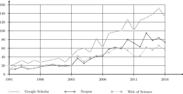
cutting and packing problems (C&PP). Wether one wants to pack a set of goods in a con-tainer, cut a set of small items from large pieces of wood, position articles in a newspaper, or even play the famous Tetris video game, they solve a C&PP. In addition, C&PP enter as a component of an incredible amount of more complex problems, such as routing problems with capacity and scheduling problems with resources constraints. It is therefore not sur-prising that researchers have focused on developing effective methods to deal with C&PP. Figure 1.1 shows the number of articles having in the title either the term bin packing, or the term cutting stock, two subclasses of C&PP, according to different bibliographic data bases, in the years 1991-2016. The picture shows the growing interest in these specific problems, with sharp increase in recent years.

As most of the problems from the C&PP family areN P-hard, see Garey and Johnson [130], they are very difficult to solve to optimality in practice and many exact approaches have been proposed in the literature, including branch-and-bound and branch-and-cut algorithms.

With the recent improvements of mixed integer linear programming (MILP) solvers (see, e.g., Achterberg and Wunderling [1] and Lodi [192]), an alternative axe of research consists in finding better MILP formulations for the problem. For example, through the last decades, no less than six different MILP models have been proposed for the classical bin packing problem: in chronological order, the textbook model by Martello and Toth [214] derived from the work of Kantorovich [167], the set covering formulation by Gilmore and Gomory [134, 135], the one-cut by Dyckoff [111], the arc-flow by Val´erio de Carvalho [278], the DP-flow by Cambazard and O’Sullivan [52], and the general arc-flow with graph compression by Brand˜ao and Pedroso [45]. A seventh, more powerful, formulation is even proposed in this thesis (Chapter 4). Vanderbeck and Wolsey [287] described in details generic procedures to obtain reformulations, and categorized them in several categories. In theextended formulations, new variables are introduced so as to better model the structure

(15)

2 Chapter 1. Introduction 0 20 40 60 80 100 120 140 160 1991 1996 2001 2006 2011 2016 * * * * * * * * _* _* _* * * * * * * * * * * * * * * _* u t ut u t u t u t u t ut u t ut u t u t u t ut u t u t u t u t ut u t u t u t u t u t u t u t u t b b b b b b b b b b b b b b b b b b b b b b b b b b

*

Scopus u

t ut _{Google Scholar} b b _{Web of Science}

Figure 1.1: Number of papers dealing with bin packing and cutting stock problems, 1991-2016

of the problem. These new variables typically allow one to model some combinatorial structure more precisely and to induce integrality through tighter linear constraints linking the variables. The reformulations that use projection allow one to reduce the number of variables so that calculations are typically faster. Some other reformulations are just

alternative formulations that aim at treating or eliminating symmetry among solutions or obtaining variables that are more effective as branching variables, or variables for which one can develop effective valid inequalities.

When the problem is very complex, which is often the case when C&PP involve two or three dimensions with non overlapping restrictions, MILP models usually struggle to find optimal solutions, as the number of variables and constraints they involve are too high. Therefore, other tools such as decomposition methods, e.g., Benders’ decomposition [34], are used. Hooker and Ottosson[157] described the Benders’ decomposition as a method that begins by partitioning the variables of a problem into two vectors x and y. It fixesy to a trial value in the master problem so as to define a slave problem that only contains x. If the solution of the slave reveals that the trial value ofy is unacceptable, the slave’s dual is used to identify a number of other values of y that are likewise unacceptable and

(16)

3

are removed from the master problem by means of cuts. The next trial value must be one that has not been excluded. Eventually only acceptable values remain, and if all goes well, the algorithm terminates after enumerating only a few of the possible values of y. In the classical Benders’ decomposition, the master is an MILP and the slave is a linear programming (LP) model. Hooker and Ottosson[157] proposed a similar decomposition called logic-based Benders decomposition, in which both the master and the subproblem are MILPs. They solved the slave problem by logical deduction methods, such as con-straint programming, whose outcome was used to produce valid cuts. Cˆot´e et al. [83] also used Benders’ decomposition where both subproblems were MILPs solved by combi-natorial algorithm. To produce effective valid cuts, they used the combicombi-natorial Benders’ cuts introduced by Codato and Fischetti [69], in which a third combinatorial algorithm is used to find the cuts that are added to the master. Note that modern implementation of Benders’ cuts involve branch-and-cut algorithms (see, e.g., Padberg and Rinaldi [228] for a description of branch-and-cut algorithms).

An alternative way to handle MILP models with too many variables is to use Dantzig-Wolfe decomposition [89]. As described by Vanderbeck [284], DantzigDantzig-Wolfe decomposition is a specific form of problem reformulation that aims at providing a tighter linear pro-gramming relaxation bound. The reformulation gives rise to an integer master problem, whose typically large number of variables is dealt by using an integer programming column generation procedure. Vance [281] showed that, when applied to the textbook model of Martello and Toth [214], the Dantzig-Wolfe decomposition leads to the set covering for-mulation of Gilmore and Gomory [134, 135]. Dantzig-Wolfe decomposition often leads to branch-and-price algorithms. As described in Barnhart et al. [23], in a branch-and-price algorithm, sets of columns are left out of the LP relaxation because there are too many columns to handle efficiently and most of them will have their associated variable equal to zero in an optimal solution anyway. Then to check the optimality of an LP solution, a subproblem, called the pricing problem, which is a separation problem for the dual LP, is solved to try to identify columns to enter the basis. If such columns are found, the LP is reoptimized. Branching occurs when no columns price out to enter the basis and the LP solution does not satisfy the integrality conditions. Branch-and-price allows column generation to be applied throughout the branch-and-bound tree.

The general scope of this thesis is to review or provide new and effective algorithms based on alternative MILP models and/or decomposition approaches to solve exactly var-ious cutting and packing problems. Each chapter of the thesis is self-contained and can

(17)

4 Chapter 1. Introduction

be read independently of the others. A unique bibliography is provided at the end of the thesis, to avoid the repetition of references.

In Chapter 2, we propose a survey on the classical bin packing and cutting stock prob-lems. After a detailed review of the literature (over 150 references), we implement and computationally test the most common methods used to solve the problems, including branch-and-price, constraint programming and mixed integer programming, and we suc-cessfully propose new sets of instances that are difficult to solve in practice.

In Chapter 3, we describe the BPPLIB, a library for bin packing and cutting stock problems. We gather the most important results from Chapter 2, test some of the algo-rithms with free solvers, and make their code publicly available. We also make additional experimental results on new sets of instances and introduce BppGame, an interactive visual solver for the bin packing problem.

In Chapter 4, we study in details the main pattern-based and pseudo-polynomial MILP formulations that have been proposed for the bin packing problems and we provide a clear picture of the dominance and equivalence relations that exist among them. In addition, we introduce a new MILP formulation for the problem and show its effectiveness through some tests on benchmark instances, achieving state of the art results and finding several new proven optimal solutions. We also show how to adapt the formulation to the variable-sized bin packing problem and the bin packing problem with item fragmentation, and obtain results that consistently improve those available in the literature.

In Chapter 5, we propose a method based on Logic based Benders’ decomposition for the orthogonal stock cutting problem and some extensions. We solve the master problem through an MILP model while constraint programming is used to solve the slave problem. The resulting method is hybridized with a state-of-the-art branch-and-bound algorithm and computational experiments on classical benchmarks from the literature show the ef-fectiveness of the proposed approach.

In Chapter 6, we compare human performances with respect to simple heuristics and exact approaches on two-dimensional packing problems. After introducing TwoBinGame, a visual application we developed for students to interactively solve two-dimensional packing problems, we detail the experimental plan we adopted to measure human efficiency when various parameters of the test instances (e.g., the number of items to pack or the possibility of rotation) change. We analyze the results obtained by about 200 students and show that the human brain is able to obtain, for relatively small instances, results comparable or better than those produced by simple heuristics such as bottom left or best fit, even when

(18)

5

coupled with powerful post-processing.

In Chapter 7, we study an optimization problem that originates from the packaging industry, in particular from the process of blown film extrusion, where a plastic film is used to produce rolls of different dimensions and colors. The film can be cut along its width, thus producing multiple rolls in parallel, and set-up times must be considered when changing from one color to another. The optimization problem that we face is to produce a given set of rolls on a number of identical parallel machines by minimizing the makespan. The problem combines cutting and scheduling decisions, and is very difficult to solve exactly. For its solution, we propose mathematical models and heuristic algorithms that involve a non-trivial decomposition method. By means of extensive computational experiments we show that proven optimality can be achieved on small instances, whereas for larger instances good quality solutions can be obtained especially by the use of an iterated local search algorithm.

In Chapter 8, we study the time-indexed formulations of the resource constrained project scheduling problem and propose some improvements based on preprocessing and lifting techniques. Then, we study the discrete time-cost tradeoff problem and introduce a new MILP model to solve the problem. Finally, we study the multi-mode resource-constrained project scheduling problem and propose a hybridized algorithm. For each of these problem, we compare the new algorithm we propose with a classical MILP formula-tion and a constraint programming approach from the literature.

(19)

(20)

Chapter 2

Bin Packing and Cutting Stock

Problems: Mathematical Models

and Exact Algorithms

1

In this chapter we review the most important mathematical models and algorithms developed for the exact solution of the one-dimensional bin packing and cutting stock problems, and experimentally evaluate, on state-of-the art computers, the performance of the main available software tools.

Keywords: Bin packing, Cutting stock, Exact algorithms, Computational evaluation.

2.1

Introduction

The (one-dimensional) bin packing problem is one of the most famous problems in combinatorial optimization. Its structure and its applications have been studied since the thirties, see Kantorovich [167]. In 1961 Gilmore and Gomory [134] introduced, for this class of problems, the concept of column generation, by deriving it from earlier ideas of Ford and Fulkerson [125] and Dantzig and Wolfe [89]. This is one of the first problems for which, since the early seventies, the worst-case performance of approximation algorithms was investigated. In the next decades lower bounds were studied and exact algorithms proposed. As the problem is strongly _{N P}-hard, many heuristic and metaheuristic approaches have also been proposed along the years.

Thebin packing problem(BPP) can be informally defined in a very simple way. We are

1_{The results of this chapter appears in: M. Delorme, M. Iori, and S. Martello, Bin Packing and Cutting}

Stock Problems: Mathematical Models and Exact Algorithms, European Journal of Operations Research, 255:1-20, 2016 [98].

(21)

8 Chapter 2. BPP and CSP: Mathematical Models and Exact Algorithms

givennitems, each having an integerweightwj (j= 1, . . . , n), and an unlimited number of

identicalbinsof integercapacityc. The objective is to pack all the items into the minimum number of bins so that the total weight packed in any bin does not exceed the capacity. (In a different but equivalent normalized definition, the weights are real numbers in [0,1], and the capacity is 1.) We assume, with no loss of generality, that 0< wj < cfor all j.

Many variants and generalizations of the BPP arise in practical contexts. One of the most important applications, studied since the sixties, is theCutting Stock Problem (CSP). Although it has been defined in different ways according to specific real world cases, its basic definition, using the BPP terminology, is as follows. We are givenmitem types, each having an integer weight wj and an integer demand dj (j = 1, . . . , m), and a sufficiently

large number of identical bins of integer capacity c. (In the CSP literature the bins are frequently calledrolls, the term coming from early applications in the paper industry, and “cutting” is normally used instead of “packing”.) The objective is to producedj copies of

each item type j (i.e., to cut/pack them) using the minimum number of bins so that the total weight in any bin does not exceed the capacity.

This chapter is devoted to a presentation of the main mathematical models that have been proposed, and to an experimental evaluation of the main available software tools that have been developed. The main motivations for writing this survey are to present, for the first time, a complete overview on these problems and to assess, through extensive computational experiments, the performance of the main computer codes that are available for their optimal solution. All the codes we evaluated are either linked or downloadable from a dedicated web page, but one that can be obtained by the authors. The same web page also provides the test instances we used, including new instances that were specifically created as challenging test cases. We believe that this study and the accompanying web page will be useful to many researchers who are still intensively studying this area. Indeed, a search on different bibliographic data bases for articles having in the title either the term ”bin packing”, or the term ”cutting stock”, or both, shows a growing interest in these problems in the last 25 years, with sharp increase in recent years (over 150 Google Scholar entries in 2015).

For exhaustive studies on specific research areas concerning the BPP and the CSP, the reader is referred to many surveys that have been published along the years. To the best of our knowledge, the following reviews have been proposed.

The first literature review on these problems was published in 1992 by Sweeney and Paternoster [270], who collected more than 400 books, articles, dissertations, and working

(22)

2.1. Introduction 9

papers appeared from 1961 to 1990. In 1990 Dyckhoff [112] proposed a typology of cutting and packing problems, and classified the BPP and the CSP as 1/V/I/M and 1/V/I/R, respectively. In the same year Martello and Toth included a chapter on the BPP in their book [214] on knapsack problems. Two years later Dyckhoff and Finke [113] published a book on cutting and packing problems arising in production and distribution, where they investigated the different structure of these problems, and classified the literature accordingly. A bibliography on the BPP has been compiled by Coffman et al. [76]. More recently, W¨ascher et al. [289] re-visited the typology by Dyckhoff [112] and proposed more detailed categorization criteria: the problems we consider are classified as 1-dimensional SBSBPP (Single Bin Size Bin Packing Problem) and 1-dimensional SSSCSP (Single Stock Size Cutting Stock Problem).

Besides the general surveys discussed above, a number of reviews concerning specific methodologies have been proposed. Already in the early eighties Garey and Johnson [131] and Coffman et al. [77] presented surveys on approximation algorithms for the BPP. Other surveys on approximation algorithms for the BPP and a number of its variants were later proposed by Coffman et al. [72, 71] and Coffman and Csirik [74]. Coffman and Csirik [73] also proposed a four-field classification scheme for papers on bin packing, aimed at highlighting the results in bin packing theory to be found in a certain article. More recently, Coffman et al. [75] presented an overview of approximation algorithms for the BPP and a number of its variants, and classified all references according to [73].

Val´erio de Carvalho [279] presented a survey of the most popularLinear Programming

(LP) methods for the BPP and the CSP. A review of models and solution methods was included by Belov [28] in his PhD thesis dedicated to one- and two-dimensional cutting stock problems.

We finally mention that extensions to higher dimensions have been investigated too. In the early nineties, Haessler and Sweeney [146] provided a description of one- and two-dimensional cutting stock problems, and a review of some of the methods to solve them. More recently, surveys on two-dimensional packing problems have been presented by Lodi et al. [193, 194, 197].

In the next section we provide a formal definition of the BPP and the CSP. In Section 2.3 we briefly review the most successful upper and lower bounding techniques for the considered problems. In Sections 2.4, 2.5, and 2.6 we examine pseudo-polynomial formu-lations, enumeration algorithms, and branch-and-price approaches, respectively. Finally, in Section 2.7, we experimentally evaluate the computational performance of twelve

(23)

com-10 Chapter 2. BPP and CSP: Mathematical Models and Exact Algorithms

puter programs available for the solution of the considered problems. Conclusions follow in Section 2.8.

2.2

Formal statement

In order to give a formal definition of the problems, let u be any upper bound on the minimum number of bins needed (for example, the value of any approximate solution), and assume that the potential bins are numbered as 1, . . . , u. By introducing two types of binary decision variables

yi =

(

1 if biniis used in the solution;

0 otherwise (i= 1, . . . , u),

xij =

(

1 if item j is packed into bin i;

0 otherwise (i= 1, . . . , u;j= 1, . . . , n),

we can model the BPP as a basic Integer Linear Program (ILP) of the form (see Martello and Toth [214]) min u X i=1 yi (2.1) s.t. n X j=1 wjxij ≤cyi (i= 1, . . . , u), (2.2) u X i=1 xij = 1 (j= 1, . . . , n), (2.3) yi ∈ {0,1} (i= 1, . . . , u), (2.4) xij ∈ {0,1} (i= 1, . . . , u;j= 1, . . . , n). (2.5)

Constraints (2.2) impose that the capacity of any used bin is not exceeded, while constraints (2.3) ensure that each item is packed into exactly one bin.

For the CSP let us defineuand yi as above, and let

(24)

2.3. Upper and lower bounds 11 The CSP is then min u X i=1 yi (2.6) s.t. m X j=1 wjξij ≤cyi (i= 1, . . . , u), (2.7) u X i=1 ξij =dj (j= 1, . . . , m), (2.8) yi∈ {0,1} (i= 1, . . . , u), (2.9) ξij ≥0,integer (i= 1, . . . , u;j = 1, . . . , m). (2.10)

The BPP can be seen as a special case of the CSP in which dj = 1 for all j. In turn, the

CSP can be modeled by a BPP in which the item set includes dj copies of each item type

j.

The BPP (and hence the CSP) has been proved to beN P-hard in the strong sense by Garey and Johnson [130] through transformation from the 3-Partition problem.

2.3

Upper and lower bounds

Most exact algorithms for bin packing problems make use of upper and lower bound computations in order to guide the search in the solution space, and to fathom partial solutions that cannot lead to optimal ones. As previously mentioned, for deep reviews on these specific domains, the reader is referred to the surveys listed in Section 2.1. In this section we briefly review the most successful upper and lower bounding techniques that have been developed, with some focus on areas for which no specific survey is available. We use the term approximation algorithm for methods for which theoretical results (like, e.g., worst-case performance) can be established, while the termheuristicdenotes methods for which the main interest relies in their practical behavior.

A classical way for evaluating upper and lower bounds is their absolute worst-case performance ratio. Given a minimization problem and an approximation algorithm A, let A(I) and OPT(I) be the solution value provided by A and the optimal solution value, respectively, for an instance I of the problem. Theworst-case performance ratio (WCPR) of Ais then defined as the smallest real number r(A)>1 such that A(I)/OP T(I) _≤r(A)

(25)

for all instances I, i.e.,

r(A) = sup

I {

A(I)/OP T(I)_}.

Similarly, the WCPR of a lower bound L is the largest real number r(L) <1 such that, for all instances I, the lower bound valueL(I) satisfiesL(I)/OP T(I)_≥r(L), i.e.,

r(L) = inf

I {L(I)/OP T(I)}.

2.3.1 Approximation algorithms

The simplest BPP approximation algorithms consider the items in any sequence. Al-gorithm Next-Fit(NF) at each iteration packs the next item into the current bin (initially, into bin 1) if it fits, or into a new bin (which becomes the current one) if it does not fit. The WCPR of NF is r(N F) = 2. Algorithm First-Fit (FF) at each iteration packs the next item into the lowest indexed bin where it fits, or into a new bin if it does not fit in any open bin. Algorithm Best-Fit(BF) at each iteration packs the next item into the feasible bin (if any) where it fits by leaving the smallest residual space, or into a new one if no open bin can accommodate it. The exact WCPR of FF and BF has been an open problem for forty years, until recently D´osa and Sgall [107, 108] proved that r(F F) =r(BF) = 17₁₀.

Better performances are obtained by preventively sorting the items according to de-creasing weight. The WCPR of the resulting algorithms First-Fit Deacreasing(FFD) and

Best-Fit decreasing (BFD) is r(F F D) =r(BF D) = 3₂ (Simchi-Levi [263]). Moreover, this is the best achievable performance, in the following sense:

Property₁ _{No polynomial-time approximation algorithm for the BPP can have a WCPR}

smaller than 3₂ unless P =N P.

Proof Consider an instance of the N P-complete Partition _{problem: is it possible} to partition S = _{w1, . . . , wn} into S1, S2 so that P_j∈S1wj =

P

j∈S2wj? Assume a

polynomial-time approximation algorithmAfor the BPP exists such thatOPT(I)> 2₃ A(I) for all instances I, and execute A for an instance ˆI of the BPP defined by (w1, . . . , wn)

and c = Pn_j=1wj/2. If A( ˆI) = 2 then we know that the answer to Partition is yes.

If instead A( Î) _≥3 then we know that OPT( Î) > 2₃3, i.e., that OPT( Î) >2, hence the answer toPartition_is_no_{. It follows that we could solve}Partition_{in polynomial time.}

Since FFD and BFD provide the best possible WCPR, most research on approximation algorithms for the BPP focused on the asymptotic WCPR, defined as the minimum real

(26)

2.3. Upper and lower bounds 13

number r∞(A) such that, for some positive integer k, A(I)/OP T(I) ≤ r∞(A) for all instances I satisfying OP T(I) _≥ k. The number of results in this area is impressive and beyond the purpose of this study: we refer the reader to the various surveys that were listed in Section 2.1. The most recent survey (2013), by Coffman et al. [75], examines 200 references from the literature. Among the papers that appeared subsequently, we mention those by D´osa et al. [106] on the FFD algorithm, by Rothvoß [242], who improved a classical result by Karmarkar and Karp [169], and by Balogh et al. [21], who closed a long standing open issue on on-line bin packing.

2.3.2 Lower bounds

To our knowledge, no general survey on lower bounds for the BPP is available. Hence we provide in the following a brief review of the corresponding literature. An obvious lower bound for the BPP, computable in O(n) time, is provided by the so-called continuous relaxation, namely L1 =     n X j=1 wj/c    , (2.11)

which gives the rounded solution value of the linear programming relaxation of (2.1)-(2.5). It is easily seen thatr(L1) = 1₂ (see, e.g., Martello and Toth [214]).

A better lower bound was obtained by Martello and Toth [215]. Given any integer α (0≤α≤c/2), let

J1={j∈N :wj > c−α};

J2={j∈N :c−α≥wj > c/2};

J3={j∈N :c/2≥wj ≥α},

and observe that each item inJ1∪J2 needs a separate bin, and that no item ofJ3can go to a

bin containing an item ofJ1. ThenL(α) =|J1|+|J2|+max

0, P j∈J3wj−(|J2|c− P j∈J2wj) c is a valid lower bound. It can be shown that the overall bound

L2 = max{L(α) : 0≤α≤c/2, α integer} (2.12)

can be computed inO(nlogn) time and has WCPR equal to 2₃. Similarly to what happens for algorithms FFD and BFD, this is the best achievable performance, namely:

(27)

Property ₂ _{No lower bound, computable in polynomial time, for the BPP can have a}

WCPR greater than 2₃ unless _P =_{N P}.

ProofWe use the same instance of Partition _{as in the proof of Property 1, and the} same induced BPP instance Î. Assume a polynomial-time lower bound L for the BPP exists such that OPT(I) < 3₂ L(I) for all instances I, and compute L for instance Î. If L( Î) _≥3 then we know that the answer to Partition _is _no_{. If} _L_{( ˆ}_I_{) = 2 then we know} that OPT( Î) < 3₂2, hence OPT( Î) = 2, i.e., that the answer to Partition _is _yes_{. We} could then solve Partition _{in polynomial time.}

Lower bounds that generalize L2 and can have better practical performance have been

proposed by Labb´e et al. [182] (lower bound L2LLM), and by Chen and Srivastava [62].

Theoretical properties of such bounds were studied by Elhedhli [117]. Bourjolly and Re-betez [44] proved that the asymptotic WCPR of the bound L2LLM proposed in [182] is

r∞(L2LLM) = 3₄.

Another lower bound, L3, dominating L2 was obtained by Martello and Toth [215]

by iteratively reducing the instance, and invoking L2 on the reduced instance. The time

complexity grows toO(n3_{), and the asymptotic WCPR is}_r∞₍_L

3) = 3₄, as proved by Crainic

et al. [85].

A different type of lower bound computation had been considered in the eighties by Lueker [203], who proposed a bounding strategy for the case where all the items are drawn from a uniform distribution, based on dual feasible functions, which were originally intro-duced by Johnson [164]. Consider the normalized definition of the BPP (see Section 2.1): a real-valued functionu(x) is called dual feasibleif, for any finite setS of nonnegative real numbers, condition P_x_∈_Sx _≤1 implies P_x_∈_Su(x) _≤1. It follows that any lower bound computed over weights u(w) is also valid for the original weightsw.

Later on, Fekete and Schepers [122] used dual feasible functions to produce new classes of fast BPP lower bounds. For example, given any normalized instanceI of the BPP, any α (0≤α≤1/2), and an item weight w, letw′ =w/c and define

U(α)₍_w′_{) =}      1 if w′ >1−α; w′ if 1₋α_≥w′ _≥α; 0 if w′ < α.

Then U(α)₍_w′_{) is a dual feasible function. (Observe in particular that, by considering all}_α values in [0,1₂] and computing the corresponding boundsL1, the maximum resulting value

(28)

2.3. Upper and lower bounds 15

A number of other dual feasible functions have been proposed in the literature. We refer the reader to Clautiaux et al. [66] and Alves et al. [9] for recent surveys on these functions and their use for the computation of BPP lower bounds.

Chao et al. [60] and Crainic et al. [86] studied methods for computing “fast” lower bounds for the BPP, i.e., bounds requiring no more than O(nlogn) time. Once a lower bound value, say ℓ, has been computed, it can sometimes be improved through additional considerations: for example, if it can be established that no feasible solution using ℓ bins exists, then ℓ+ 1 is a valid lower bound value. Improvement techniques of this kind have been studied by Dell’Amico and Martello [95], Alvim et al. [11], Haouari and Gharbi [147], and Jarboui et al. [163].

Other effective lower bounds, which however require a non-polynomial time, including the famous Gilmore-Gomory column generation method, are discussed in Section 2.6.

2.3.3 Heuristics and metaheuristics

The focus of this chapter is on the optimal solution of bin packing and cutting stock problems. Approximate and heuristic solutions have thus marginal interest here, but they are commonly used to provide an initial solution to exact algorithms. For the sake of completeness, in this section we briefly review a number of heuristic and metaheuristic approaches.

Heuristics

The first relevant contribution of this kind is probably the one by Eilon and Christofides [114] who presented a heuristic for a number of packing problems, basically consisting of algorithm BFD (see Section 2.3.1), plus a reshuffle routine when the solution is not equal to the continuous relaxation L1. Roodman [239] presented a set of heuristics for variants

of the CSP, mainly based on an initial greedy solution improved through local search. Vahrenkamp [277] proposed a random search for the CSP, based on a heuristic developed by Haessler [145] for generating cutting patterns for trim problems. W¨ascher and Gau [288] considered a generalization of the CSP, and studied the computational behavior of heuristics based on rounding the solutions obtained from the LP relaxation of a generalization of the Gilmore and Gomory [134] model (see Section 2.6). The experiments were performed on random instances produced by their generator, CUTGEN (see Gau and W¨ascher [132]), which creates CSP instances depending on five parameters: number of item types, minimum and maximum weight, bin capacity, and average demand.

(29)

Gupta and Ho [143] proposed a heuristic algorithm based on the minimization of the unused bin capacities, and successfully compared it with FFD and BFD (although at the expenses of higher CPU times). Mukhacheva et al. [222] presented a modified FFD algo-rithm which was later embedded in the exact algoalgo-rithm by Belov and Scheithauer [30] (see Section 2.6.3). Osogami and Okano [226] proposed variants of some classical approximation algorithms, and investigated the effect of a local search based on item exchanges. Other modifications of classical approximation algorithms were proposed by Bhatia et al. [40], Kim and Wy [173], and Fleszar and Charalambous [123]. The effectiveness of a hill climb-ing local search strategy for the BPP, also based on item exchanges, was later investigated by Lewis [187].

As for most_{N P}-hard problems, starting from the early nineties many metaheuristic ap-proaches of all kinds have been proposed for the BPP and the CSP. In the following, we list, grouped by metaheuristic paradigm, a number of contributions that provided interesting insights into the problems at hand.

Simulated annealing and Tabu search

A classical simulated annealing approach to the BPP was implemented by K¨ampke [166], while a variant of the method (called weight annealing) was proposed by Loh et al. [199]. Scholl et al. [251] used a Tabu search procedure to speed up their well-known exact algorithm (BISON) for the BPP, treated in Section 2.5.1. Alvim et al. [11] embedded a Tabu search in a hybrid improvement heuristic for the BPP.

Population based algorithms

Probably, the first genetic approach to the BPP is the one by Falkenauer and Delcham-bre [120]: they showed that the classical genetic approach cannot work efficiently for certain kinds of problems (like the BPP), and presented a variant (the grouping genetic algo-rithm) capable of producing a good computational behavior. Falkenauer [119] improved this method through hybridization with the dominance criterion by Martello and Toth [215] (see Section 2.5.1), and proposed a set of benchmark instances that was later adopted by many authors for computationally testing BPP algorithms. Although Gent [133] showed that the majority of them are very easy, these instances were used, e.g., for testing the genetic approaches by Reeves [235], Bhatia and Basu [39], Singh and Gupta [264], ¨Ulker et al. [276], and Stawowy [267]. Other genetic algorithms were proposed by Poli et al. [230] and by Rohlfshagen and Bullinaria [237, 238]. Recently, a very effective genetic algorithm

(30)

2.4. Pseudo-polynomial formulations 17

was proposed by Quiroz-Castellanos et al. [233].

Levine and Ducatelle [186] used an ant colony approach combined with a local search to solve the BPP. Liang et al. [188] proposed an evolutionary programming algorithm for the CSP and some of its variants.

Hyper-heuristics

Ross et al. [240, 241] attacked the BPP through combinations of genetic algorithms and hyper-heuristics. Other combinations of evolutionary algorithms and hyper-heuristics for the BPP were proposed by L´opez-Camacho et al. [200], Sim et al. [262], and Burke et al. [50].

Bai et al. [17] tested on BPP instances their simulated annealing hyper-heuristic ap-proach. Sim and Heart [261] used genetic programming as a generative hyper-heuristic to create deterministic heuristics.

Other meta-heuristic approaches

Fleszar and Hindi [124] obtained new heuristics for the BPP by modifying the heuristic of Gupta and Ho [143] and proposed a variable neighborhood search algorithm. G´ omez-Meneses and Randall [137] proposed a hybrid extremal optimization approach with local search for the BPP.

2.4

Pseudo-polynomial formulations

In this section we introduce considerations on polynomial and pseudo-polynomial mod-els, we present the main pseudo-polynomial formulations proposed in the literature, and highlight some relations among them.

2.4.1 Considerations on the basic ILP model

The textbook BPP model (2.1)–(2.5), which has its roots in the seminal work by Kan-torovich [167], was formally defined in 1990 by Martello and Toth [214]. It involves a polynomial number of variables and constraints but is not very efficient in practice, as shown in Section 2.7. Several attempts have been made since then to try and improve the computational behavior of the model, especially by providing families of valid inequalities. The simple inequality yi ≥ yi+1 for i = 1, . . . , u−1 reduces the size of the enumeration

(31)

can be further removed by setting xij = 0 for all j = 1, . . . , u−1 and i = j+ 1, . . . , u,

as there is always an optimal solution in which item 1 is packed in bin 1, item 2 either in bin 1 or 2, and so on. The linear relaxation of the model can be further strengthened by imposing that full items cannot be packed into binsiwith fractionalyi value, i.e.,xij ≤yi

for alli= 1, . . . , uand j= 1, . . . , n. A number of enhanced families of inequalities, includ-ing the well-known cover inequalities and their generalizations, derive from studies on the knapsack polytope. For a detailed description of these inequalities, as well as of efficient separation procedures, we refer the reader to Gabrel and Minoux [128] and Kaparis and Letchford [168].

Despite these results, the computational behavior of model (2.1)–(2.5) remains quite poor. The literature has consequently focused on the study of models with better compu-tational performance, including pseudo-polynomialmodels. The drawback of these models is that the number of variables depends not only on the number of items but also on the bin capacity. On the other hand, they provide a stronger linear relaxation than that given by (2.1)–(2.5).

In Section 2.4.2 we address the oldest such model, independently developed by Rao [234] in 1976 and by Dyckhoff [111] few years later. The most relevant approach of this kind (somehow anticipated by Wolsey [293] in 1977) was presented in 1999 by Val´erio de Carvalho [278] for the CSP. In 2010, Cambazard and O’Sullivan [52] presented a BPP pseudo-polynomial model based on a similar idea, but described in a form inspired by the graph construction used by Trick [274] for propagating knapsack constraints. We anticipate its description in Section 2.4.3, since this makes it easier to understand the Val´erio de Carvalho model, which is then discussed in Section 2.4.4 together with a recently proposed variant.

(32)

The following example is resumed a number of times in the next sections.

Example₁ _{For the BPP, we consider an instance with}_n_{= 6}_,_c_{= 9}_{, and}_w_{= (4}_,₄_,₃_,₃_,₂_,₂₎_.

The equivalent CSP instance has m= 3, c= 9, w= (4,3,2), and d= (2,2,2). An optimal solution has value 2, and packs three items (of weight 4, 3, and 2) in each bin.

2.4.2 One-cut formulation

The idea behind the Rao [234] and Dyckhoff [111] model for the CSP is to simulate the physical cutting process, by first dividing an ideal bin into two pieces (left and right), where the left piece is an item that has been cut, while the right piece is either a residual that can be re-used to produce other items or it is another item. The process is iterated on cutting residuals or new bins, until all demands are fulfilled. For the sake of clarity, we use in this section the term “width” for “weight”.

LetW ={w1, w2, . . . , wm} be the set of item widths. LetR be the set of all possible

relevant residual widths, computed by subtracting from the bin capacity c all feasible combinations of item widths (including the empty combination), provided the resulting value is not less than the minimum item width. Formally,

R=_{c₋w¯: ¯w= m X j=1 wjxj,w¯≤c−min j {wj}, xj ∈ {0,1, . . . , bj}(j= 1. . . . , m)}.

The level of demand for a certain widthq is

Lq=

(

di if q=wi for some item typei;

0 otherwise. (q∈W ∪R).

Additionally, for each q_∈W _∪R, let

• A(q) = {p ∈ R :p > q} if q ∈W (and A(q) =∅ otherwise) denote the set of piece widths that can be used for producing a left piece (item) of widthq,

• B(q) =_{p_∈W :p+q_∈R_}denote the set of item widths that, if cut as a left piece, would leave a right piece (residual) of widthq, and

• C(q) =_{p_∈W :p < q_}denote the set of item widths that can be cut, as a left piece, from a residual of widthq.

(33)

By introducing an integer variable xpq, that gives the number of times a bin, or a

residual of width p, is cut into a left piece of width q and a right piece of width p₋q (p∈R, q∈W, p > q), theone-cutmodel can be defined as the ILP

min X q∈W xcq (2.13) s.t. X p∈A(q) xpq+ X p∈B(q) xp+q,p≥Lq+ X r∈C(q) xqr q∈(W ∪R)\{c}, (2.14) xpq≥0 and integer p∈R, q∈W, p > q. (2.15)

The objective function (2.13) minimizes the number of times an item is cut from a bin. Constraints (2.14) impose that, for each widthq, the sum of the left pieces of widthq plus the sum of the right pieces of width q is not smaller than the level of demand of width q plus the number of times a residual of width q is used to produce smaller items.

Example_{1 (resumed)}_{For the CSP instance we have}_W₌_{₂_,₃_,₄_}_and_R₌_{₂_,₃_,₄_,₅_,₆_,₇_,₉_}_.

We obtain: • A(2) = {3,4,5,6,7,9}, A(3) = {4,5,6,7,9}, A(4) = {5,6,7,9}, A(5) = A(6) = A(7) =A(9) =_∅; • B(2) = B(3) = _{2,3,4_}, B(4) = _{2,3_}, B(5) = _{2,4_}, B(6) = _{3_}, B(7) = {2_}, B(9) =_∅; • C(2) =_∅, C(3) =_{2_}, C(4) =_{2,3_}, C(5) =C(6) =C(7) =C(9) =_{2,3,4_}. An optimal solution is then given by x9,4 = 2, x5,3 = 2, and xpq = 0 otherwise. In other words, we cut two items of width 4 from two bins, and two items of width 3 from the two residuals we have obtained. The two resulting residuals provide two items of width 2.

Set R can be obtained by running a standard dynamic programming algorithm, or a recursive algorithm, that generates all possible item combinations. The one-cut model (2.13)-(2.15) has O(mc) variables andO(c) constraints.

Stadtler [266] studied the combinatorial structure of the one-cut model and extended it by including additional variables and constraints. He also worked on comparing the model and the classical column generation approach, and concluded that “The set of real world cutting stock problems solvable by the one-cut model (of Rao and Dyckhoff) is only

(34)

a subset of those which could be tackled by the column generation approach (of Gilmore and Gomory)”.

2.4.3 DP-flow formulation

A simple pseudo-polynomial model is obtained by associating variables to the decisions taken in a classical dynamic programming (DP) table. In the BPP model proposed by Cambazard and O’Sullivan [52], known as DP-flow, the DP states are represented by a graph in which a path that starts from an initial node and ends at a terminal node represents a feasible filling of a bin. Let us denote by (j, d) (j = 0, . . . , n andd= 0, . . . , c) a DP state in which decisions have been taken up to item j and result in a partial bin fillingofdunits. Let us also denote by ((j, d),(j+ 1, e)) an arc connecting states (j, d) and (j+ 1, e). Such arc expresses the decision on whether packing or not item j+ 1 starting from the current state (j, d): the state reached by the arc is (j+ 1, d+wj+1) if itemj+ 1

is packed, and (j+ 1, d) otherwise.

Example _{1 (resumed)} _{The DP table associated with our instance is shown in Figure 2.1,}

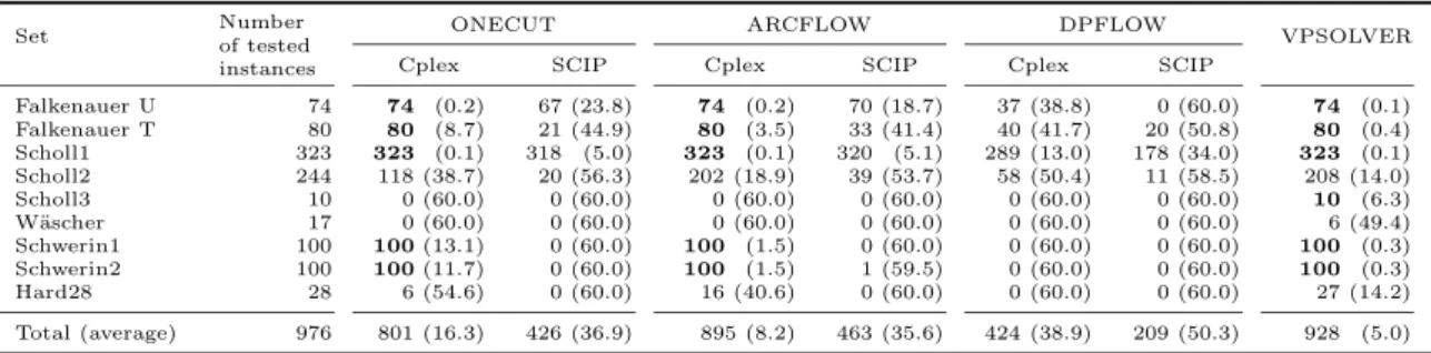
where states are represented by nodes and organized in n+ 1 horizontal layers. The table includes an additional terminal state (n+ 1, c), and states in layer n are connected to it by loss arcs (dashed lines), that express the amount of unused capacity in a given bin.

Let A denote the set of all arcs. As a feasible bin filling is represented by a path that starts from node (0,0) and ends at node (n+ 1, c), the BPP is to select the minimum number of paths that contain all items. To formulate this decision problem, let us associate an integer variablexj,d,j+1,e to arc ((j, d),(j+ 1, e))∈A, representing the number of times

the arc has been chosen to form paths. Let δ−((j, d)) (resp. δ+₍₍_{j, d}_{))) denote the set of}

arcs entering (resp. emanating from) state (j, d). The BPP can be then modeled as

min z (2.16) s.t. X ((j,d),(j+1,e))∈δ+_((j,d)) xj,d,j+1,e− X ((j−1,e),(j,d))∈δ−_((j,d)) xj−1,e,j,d=      z if (j, d) = (0,0); −z if (j, d) = (n+ 1, c); 0 otherwise, (2.17) X ((j−1,d),(j,d+wj))∈A xj−1,d,j,d+wj = 1 (j = 1, . . . , n), (2.18)

(35)

22 Chapter 2. BPP and CSP: Mathematical Models and Exact Algorithms 0,0 1,0 2,0 3,0 4,0 5,0 6,0 1,4 2,4 3,4 4,4 5,4 6,4 2,8 3,8 4,8 5,8 6,8 3,3 4,3 5,3 6,3 3,7 4,7 5,7 6,7 4,6 5,6 6,6 5,9 6,9 5,2 6,2 5,5 6,5 7,9 Figure 2.1: DP-flow graph construction for Example 1

xj,d,j+1,e≥0 and integer ((j, d),(j+ 1, e))∈A. (2.19)

The objective function (2.16) minimizes the number of bins. Constraints (2.17) impose the flow (number of bins) conservation at all nodes, while constraints (2.18) ensure that each item is packed exactly once. Note that a “≥” sign could be used in (2.18) without affecting the correctness of the model.

Example 1 (resumed) For the BPP instance an optimal solution is produced by the two paths highlighted in Figure 2.1, namely [(0,0), (1,4), (2,4), (3,7), (4,7), (5,9), (6,9), (7,9)]

and [(0,0), (1,0), (2,4), (3,4), (4,7), (5,7), (6,9), (7,9)].

The DP-flow model (2.16)-(2.19) hasO(nc) variables and constraints. This formulation was developed in [52] for the BPP, but it could be extended to the CSP. The formulations

(36)

introduced in the next section were instead specifically tailored on the CSP.

2.4.4 Arc-flow formulations

An effective CSP pseudo-polynomial formulation, denoted arc-flow, was presented by Val´erio de Carvalho [278], who used it in a branch-and-price algorithm (see Section 2.6). To make its comprehension easier, consider again Example 1, and the DP representation depicted in Figure 2.1. Now imagine that the graph is vertically shrunk, by grouping all states with the same partial bin filling into a single one. In this way, the “vertical” arcs disappear, while the “slanting” ones that connect the same pair of nodes merge into a single arc. Figure 2.2 shows the counterpart of Figure 2.1. Note that the loss arcs, which imply no bin filling variation, connect here consecutive nodes instead of (equivalently) going to the terminal node. Let A′ denote the resulting arc set, and xde the number of times arc

(d, e)∈A′ is chosen. The filling of a single bin corresponds to a path from node 0 to node c in this graph. The CSP can then be modeled as the following ILP:

min z (2.20) s.t. ₋ X (d,e)∈δ−_(e) xde+ X (e,f)∈δ+_(e) xef =      z if e= 0; −z fore=c; 0 otherwise, (2.21) X (d,d+wi)∈A′ xd,d+wi ≥bi (i= 1, . . . , m), (2.22) xde ≥0 and integer (d, e)∈A′, (2.23)

where δ−(e) (resp. δ+(e)) denotes the set of arcs entering (resp. emanating from)e. Constraints (2.21) impose the flow conservation at all nodes. Constraints (2.22) impose that, for each item typei, at least bi arcs of length wi are used, i.e., that at least bi copies

of item type iare packed.

0 2 3 4 5 6 7 8 9

(37)

Example _{1 (resumed)} _{An optimal solution to the CSP instance consists of two identical}

paths [0,4,7,9], highlighted in Figure 2.2.

The arc-flow model (2.20)-(2.23) hasO(mc) variables andO(m+c) constraints. Val´erio de Carvalho [278] proposed however a number of improvements to the above basic model, aimed at reducing the number of arcs. For example (see again Figure 2.2), it is enough to only create nodes that correspond to feasible combinations of item weights. In addition, it is proved in [278] that the linear programming relaxation of (2.20)-(2.23) has the same solution value as the Gilmore and Gomory [134] model (see Section 2.6).

Very recently, Brand˜ao and Pedroso [45] proposed an alternative CSP arc-flow formu-lation. They start with a multi-graph generalization of the arc-flow formulation by Val´erio de Carvalho [278] which uses a level per item type and can be seen as a CSP version of the DP-flow formulation. A three-index variable, sayxdei, is consequently associated with each

arc (d, e, i), wheredandeare the tail and the head, while irepresents the item type. This leads to a three-index model analogous to (2.20)-(2.23) in which, however, those inequality constraints (2.22) for which bi = 1 are changed to equalities. The resulting graph is then

reduced through graph compression techniques, and solved through a standard ILP solver. The overall code (see Section 2.7) proved to be very efficient on benchmark instances.

2.5

Enumeration algorithms

The first attempts to exactly solve the BPP and the CSP were developed in the fifties and in the sixties using LP relaxations and dynamic programming (see Eisemann [115] and Gilmore and Gomory [134, 135, 136]). Starting from the early seventies, research in this field focused on branch-and-bound.

2.5.1 Branch-and-bound

To the best of our knowledge, the first branch-and-bound algorithm for the BPP was proposed by Elion and Christofides [114], who adapted the general enumerative scheme proposed by Balas [19] for solving LPs with zero-one variables. Their algorithm produces a binary decision tree in which a node generates two descendant nodes by assigning a certain item to a certain bin, or by excluding it from that bin. The process is initialized by the heuristic solution produced by the BFD algorithm (see Section 2.3.1) followed by a reshuffle

(38)

2.5. Enumeration algorithms 25

routine. Lower bounds are obtained from a standard LP relaxation. The algorithm could only solve instances of very moderate size.

Later on, thanks to the development of better heuristics, improved lower bounds, and reduction procedures, a more powerful branch-and-bound algorithm for the BPP, called MTP, was developed by Martello and Toth [214]. During the nineties, this algorithm, whose Fortran code was available, has been the standard reference for the exact solution of the BPP. Their reduction procedures, which were later adopted by several authors, are based on the following dominance criterion. Given an instance I of the BPP, define a

feasible setF as a set of items such thatP_j_∈_Fwj ≤c. A feasible setF1 dominatesanother

feasible set F2 if the optimal solution obtained by imposing F1 as the content of a bin is

not greater than that obtained by imposingF2 as the content of a bin. Martello and Toth

[215] proved the following

Property ₃ _{Given two distinct feasible sets} _F₁ _and _F₂_{, if there exists a partition} _P ₌

{P1, . . . , Pℓ} of F2, and a subset {j1, . . . , jℓ} of F1 such that wjh ≥

P

k∈Phwk for h =

1, . . . , ℓ, then F1 dominates F2.

Clearly, if a feasible setF containing an itemjdominates all other feasible sets contain-ing the same item j, then we can imposeF to a bin and reduce the instance accordingly. Checking all such sets is computationally too heavy, and hence the Martello-Toth reduc-tion procedureMTRP limits the search to feasible sets of cardinality at most three and has O(n2) time complexity. The procedure was also used (iteratively) to produce, in O(n3) time, an improved lower bound L3. Algorithm MTP sorts the items according to

non-increasing weight, and indexes the bins according to the order in which they are initialized: at each decision node, the next free item is assigned, in turn, to all initialized bins that can accommodate it, and to a new bin. The branch-decision tree is searched according to a depth-first strategy.

Some years after the development of MTP, Scholl et al. [251] proposed the other most successful branch-and-bound algorithm for the BPP, known as BISON. They adopted some of the most powerful tools from MTP, and added new lower bounds and emerging techniques like Tabu search, obtaining an improved exact method for the BPP. A couple of years later, Schwerin and W¨ascher [255] improved the competitiveness of MTP with respect to BISON through a lower bound provided by the column generation method developed by Gilmore and Gomory [134] (see Section 2.6) for the CSP.

(39)

In the early noughties Mukhacheva et al. [222] proposed a pattern oriented branch-and-bound algorithm for both the BPP and the CSP, while Korf [179, 180] proposed a “bin completion” algorithm (later improved on by Schreiber and Korf [252]) in which decision nodes are produced by assigning a feasible set to a bin. However, starting from the late nineties, branch-and-price (see Section 2.6) proved to be very effective, and became the most popular choice for the exact solution of the BPP. Tree search enumeration is also an ingredient of constraint programming approaches, that are briefly examined in the next section.

2.5.2 Constraint programming approaches

In the last decade some attempts have been proposed to solve the BPP through Con-straint Programming (CP). Shaw [257] presented a new dedicated constraint (later on implemented in the CP optimizer of CPLEX as IloPack) based on a set of pruning and propagation rules that also make use of lower bound L2. In the following years, some

improvements on Shaw’s constraint were proposed. Cambazard and O’Sullivan [52] inte-grated pseudo-polynomial formulations discussed in Section 2.4 within the CP approach by Shaw. Dupuis et al. [110] used lower boundL2LLM by Labb´e et al. [182] and an additional

reduction algorithm. Schaus et al. [245] introduced a filtering rule based on cardinality considerations.

2.6

Branch-and-price

The Branch-and-Pricealgorithms for the BPP and the CSP are based on the seminal work by Gilmore and Gomory [134, 135], who presented the classical set covering formula-tion for the CSP, and showed how to solve its continuous relaxaformula-tion by means of acolumn generation approach. Although the branch-and-price approach could be used to solve all the models of Section 2.4, to the best of our knowledge, in the BPP and CSP literature it was mainly adopted for Gilmore-Gomory formulations, and hence our description follows such model.

2.6.1 Set covering formulation and column generation

The set covering formulation is based on the enumeration of all patterns, i.e., of all combinations of items that can fit into a bin. For the sake of conciseness, in the following

(40)

2.6. Branch-and-price 27

we use p to define both a pattern and its index, and P to define both the set of patterns and the set of patterns indices.

For the CSP, a pattern p is described by an integer array (a1p, a2p, . . . , amp), where

ajp gives the number of copies of item j that are contained in pattern p, and satisfies

Pm

j=1ajpwj ≤c, and ajp ≥0, integer (j = 1, . . . , m). Let us introduce an integer variable

yp that gives, for each p ∈ P, the number of times pattern p is used. The set covering

formulation of the CSP is given by the ILP

min X p∈P yp (2.24) s.t. X p∈P ajpyp ≥dj (j = 1, . . . , m), (2.25) yp≥0 and integer (p∈P). (2.26)

Objective function (2.24) requires the minimization of the number of bins, whereas con-straints (2.25) impose that the subset of selected patterns contains at least dj copies of

each itemj.

Similarly, for the BPP: (i) a pattern p is defined by a binary array (a1p, a2p, . . . , anp),

whereajpis equal to 1 if itemjis contained in patternpand 0 otherwise; (ii)ypis a decision

variable taking the value 1 iff patternpis used in the solution. The set covering formulation is then obtained by modifying (2.25) and (2.26) as P_p_∈_Pajpyp ≥ 1 (j = 1, . . . , n) and

yp ∈ {0,1}(p∈P), respectively.

Contrary to what happens with pseudo-polynomial models, in these formulations the number of feasible patterns is exponential in the number of items, so enumerating all of them is prohibitive even for moderate-size instances. Column generation techniques are consequently adopted for these cases, while they are less frequent for the other models. Let us briefly describe the basic technique for the CSP. We first define the continuous relaxation of (2.24)-(2.26) by removing the integrality constraints, and heuristically initialize it with a reduced set of patternsP′ _⊆P that provides a feasible solution. The resulting optimization problem, called the restricted master problem(RMP), is

min X p∈P′ yp (2.27) s.t. X p∈P′ ajpyp≥dj (j = 1, . . . , m), (2.28)

(41)

yp ≥0 (p∈P′). (2.29)

Once (2.27)-(2.29) has been solved, let πj be the dual variable associated with the jth

constraint (2.28). The existence of a column p 6∈ P′ that could reduce the objective function value (pricing problem) is determined by thereduced costscp =