TOWARD ROBUST GROUP-WISE EQTL MAPPING VIA INTEGRATING MULTI-DOMAIN HETEROGENEOUS DATA
Wei Cheng
A dissertation submitted to the faculty of the University of North Carolina at Chapel Hill in partial fulfillment of the requirements for the degree of Doctor of Philosophy in the Department of
Computer Science.
Chapel Hill 2015
Approved by: Wei Wang Wei Sun
© 2015 Wei Cheng
ABSTRACT
Wei Cheng: Toward Robust Group-Wise eQTL Mapping via Integrating Multi-Domain Heterogeneous Data
(Under the direction of Wei Wang)
As a promising tool for dissecting the genetic basis of common diseases, expression quantitative trait loci (eQTL) study has attracted increasing research interest. Traditional eQTL methods focus on testing the associations between individual single-nucleotide polymorphisms (SNPs) and gene expression traits. A major drawback of this approach is that it cannot model the joint effect of a set of SNPs on a set of genes, which may correspond to biological pathways. This thesis studies the problem of identifying group-wise associations in eQTL mapping. Based on the intuition of group-wise association, we examine how the integration of heterogeneous prior knowledge on the correlation structures between SNPs, and between genes can improve the robustness and the interpretability of eQTL mapping. To obtain a more accurate knowledgebase on the interactions among SNPs and genes, we developed a robust and flexible approach that can incorporate multiple data sources and automatically identify noisy sources. Extensive
ACKNOWLEDGEMENTS
First of all, I would like to express my sincere gratefulness to my advisor, Dr. Wei Wang, for her continuous guidance and support. I feel especially fortunate to have worked closely with Dr. Patrick Sullivan and Dr. Xiang Zhang, who encouraged me to work persistently and greatly helped me to improve my critical thinking ability and writing skill. Special thanks go to Dr. Leonard McMillan who chaired my committee and provided assistance to me. I would also like to thank Dr. Wei Sun and Dr. Marc Niethammer, who served on my committee and devoted a lot of effort to my study.
My special thanks also go to members of CompGen Lab, including Eric Yi Liu, Zhaojun Zhang, Shunping Huang, Weibo Wang, and others, for their thoughtful discussions on the problems in the research. I would like to thank all fellow persons I met in the Computer Science department who provided all kinds of help to me during my entire pursuit of PhD. I would also like to thank all the warm-hearted persons I met in the past few years for helping me to live in Chapel Hill, the beautiful town in North Carolina.
TABLE OF CONTENTS
LIST OF TABLES . . . x
LIST OF FIGURES . . . xi
1 INTRODUCTION . . . 1
1.1 eQTL Mapping . . . 2
1.2 Group-Wise eQTL Mapping and Challenges . . . 4
1.3 Thesis Statement . . . 5
1.4 Overview of the Developed Algorithms . . . 6
1.5 Thesis Outline. . . 8
2 GROUP-WISE EQTL MAPPING . . . 9
2.1 Introduction . . . 9
2.2 Related Work . . . 11
2.3 The Problem . . . 12
2.4 Detecting Group-Wise Associations . . . 13
2.4.1 SET-eQTL Model . . . 13
2.4.2 Objective Function . . . 14
2.5 Considering Confounding Factors . . . 20
2.6 Incorporating Individual Effect . . . 20
2.6.1 Objective Function . . . 21
2.6.2 Increasing Computational Speed . . . 25
2.6.2.1 Updatingσ2. . . 26
2.6.2.3 Preparation for Derivatives ofO for Model 2 . . . 27
2.6.2.4 Proof of Theorem 1 . . . 28
2.7 Optimization . . . 29
2.8 Experimental Results . . . 30
2.8.1 Simulation Study . . . 30
2.8.1.1 Shrinkage ofCandB×A . . . 32
2.8.1.2 Computational Efficiency Evaluation . . . 33
2.8.2 Yeast eQTL Study . . . 34
2.8.2.1 cis- and trans- Enrichment Analysis . . . 36
2.8.2.2 Reproducibility of trans Regulatory Hotspots between Studies . . . . 38
2.8.2.3 Gene Ontology Enrichment Analysis . . . 39
2.9 Conclusion . . . 41
3 REFINING PRIOR GROUPING INFORMATION . . . 45
3.1 Introduction . . . 45
3.2 The Problem . . . 47
3.3 Co-Regularized Multi-Domain Graph Clustering . . . 48
3.3.1 Objective Function . . . 48
3.3.1.1 Single-Domain Clustering . . . 48
3.3.1.2 Cross-Domain Co-Regularization . . . 49
3.3.1.3 Joint Matrix Optimization . . . 51
3.3.2 Learning Algorithm . . . 51
3.3.3 Theoretical Analysis . . . 52
3.3.3.1 Derivation . . . 52
3.3.3.2 Convergence . . . 54
3.3.3.3 Complexity Analysis . . . 55
3.3.4 Finding Global Optimum . . . 55
3.3.4.2 Lower Bound of Termination Thresholdcϕ . . . 56
3.3.4.3 Parallelizing the Global Optimum Search Process . . . 57
3.3.5 Re-Evaluating Cross-Domain Relationship . . . 58
3.3.6 Assigning Optimal Weights Associated with Focused Domain . . . 59
3.4 Experimental Results . . . 63
3.4.1 Effectiveness Evaluation . . . 63
3.4.2 Robustness Evaluation . . . 65
3.4.3 Binary v.s. Weighted Relationship . . . 66
3.4.4 Evaluation of Assigning Optimalλ’s Associated with Focused Domain . . . 68
3.4.5 Protein Module Detection by Integrating Multi-Domain Heterogenous Data 69 3.4.6 Performance Evaluation . . . 75
3.5 Conclusion . . . 76
4 INCORPORATING PRIOR GROUPING KNOWLEDGE . . . 77
4.1 Introduction . . . 77
4.2 Background: Linear Regression with Graph Regularizer . . . 80
4.2.1 Lasso and LORS . . . 81
4.2.2 Graph-regularized Lasso . . . 81
4.3 Graph-regularized Dual Lasso . . . 83
4.3.1 Optimization: An Alternating Minimization Approach . . . 83
4.3.2 Convergence Analysis . . . 86
4.4 Generalized Graph-regularized Dual Lasso . . . 89
4.5 Experimental Results . . . 92
4.5.1 Simulation Study . . . 92
4.5.2 Yeast eQTL Study . . . 96
4.5.2.1 cis and trans Enrichment Analysis . . . 96
4.6 Conclusion . . . 102
5 DISCUSSION . . . 103
5.1 Summary . . . 104
5.2 Future Directions . . . 105
LIST OF TABLES
2.1 Summary of Notations . . . 12
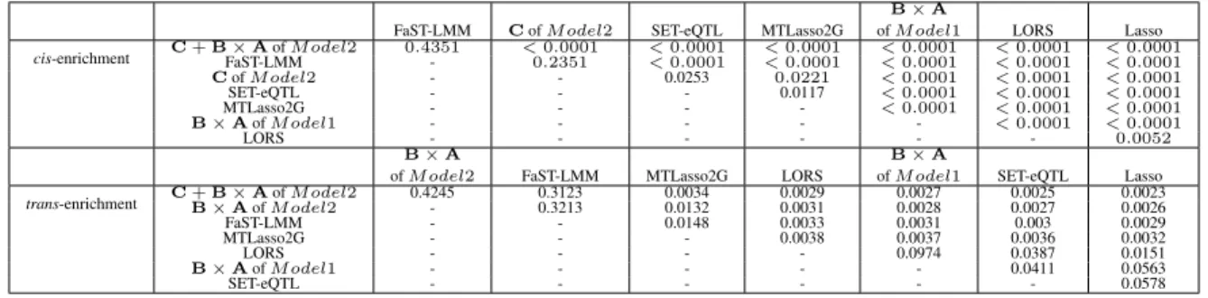
2.2 Pairwise comparison of different models usingcis- andtrans- enrichment. . . 37
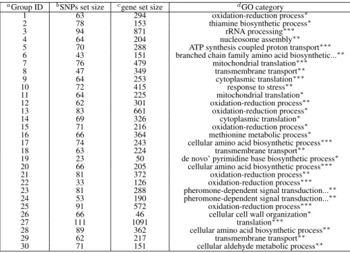
2.3 Summary of all detected groups of genes fromM odel2on yeast data. . . 41
2.4 Summary of detected significantly enriched gene groups fromM odel1(Part I). . . 42
2.5 Summary of detected significantly enriched gene groups fromM odel1(Part II). . . . 43
2.6 Summary of the top 15 detected hotspots by LORS. . . 43
2.7 Summary of detected significantly enriched gene groups from SET-eQTL. . . 44
3.1 Summary of symbols and their meanings . . . 48
3.2 Population size and termination threshold for the Tabu search algorithm . . . 57
3.3 The UCI benchmarks . . . 63
3.4 The newsgroup data . . . 66
3.5 GO enrichment analysis of the gene sets identified by different methods . . . 73
3.6 Number of identified protein modules by different methods. . . 73
3.7 Running time on different data sets . . . 76
4.1 Summary of Notations . . . 80
4.2 Pairwise comparison of different models usingcis- andtrans- enrichment. . . 97
4.3 Summary of the top-15 hotspots detected by GGD-Lasso. . . 99
4.4 Hotspots detected by different methods . . . 99
4.5 Summary of the top 15 detected hotspots by GD-Lasso . . . 101
4.6 Summary of the top 15 detected hotspots by G-Lasso. . . 101
LIST OF FIGURES
1.1 An example dataset in eQTL mapping . . . 2
1.2 Examples of associations between a gene expression level and two different SNPs . . 3
1.3 Association weights estimated by Lasso on the example data . . . 4
1.4 An illustration of individual and group-wise associations. . . 5
2.1 The proposed graphical model with hidden variables . . . 14
2.2 An example of the inferred sparse graphical model . . . 14
2.3 Graphical model with two types of hidden variables . . . 20
2.4 Refined graphical model to capture both individual and group-wise associations. . . . 21
2.5 Ground truth ofβand linkage weights estimated byM odel2on simulated data. . . . 31
2.6 Association weights estimated byM odel1andM odel2. . . 31
2.7 The ROC curve of FPR-TPR on simulated data. . . 32
2.8 The areas under the precision-recall/FPR-TPR curve (AUCs). . . 32
2.9 Model 2 shrinkage of coefficients forB×AandCrespectively. . . 33
2.10 Running time performance on simulated data when varyingN andM. . . 34
2.11 Parameter tuning forM andH(M odel2) . . . 35
2.12 Significant associations discovered by different methods in yeast. . . 36
2.13 Consistency of detected eQTL hotspots . . . 38
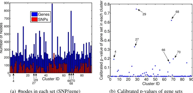
2.14 Number of nodes and calibratedp-values in each group-wise association . . . 40
2.15 Number of SNPs and genes in each group-wise association. . . 40
3.1 Multi-view graph clustering vs co-regularized multi-domain graph clustering (CGC) 46 3.2 Focused domainπand 5 domains related to it . . . 59
3.3 Clustering results on UCI datasets(Wine v.s. Iris, Ionosphere v.s. WDBC) . . . 64
3.4 Clustering with inconsistent cross-domain relationship . . . 65
3.6 Binary and weighted relationship matrices . . . 67
3.7 Clustering results on the newsgroup data set with binary or weighted relationships . . 68
3.8 Clustering accuracy of the auxiliary(1–5) and the focused domains (γ = 0.05) . . . 69
3.9 Optimal weights (λr) and the correspondingµr (γ = 0.05) . . . 70
3.10 Clustering accuracy of auxiliary domains 1–5 and the focused domain (γ = 0.1) . . . . 70
3.11 Optimal weights (λr) of auxiliary domains 1–5 with differentγ . . . 70
3.12 PPI network, gene co-expression network, genetic interaction network. . . 71
3.13 Two star networks for inferring optimal weights . . . 72
3.14 Comparison of CGC and single-domain graph clustering (k= 100) . . . 74
3.15 Number of iterations to converge (CGC) . . . 74
3.16 Objective function values of 100 runs with random initializations (newsgroup data) . 74 3.17 Number of runs used for finding global optima . . . 75
4.1 Examples of prior knowledge onSandG. . . 79
4.2 Ground truth ofWand that estimated by different methods. . . 92
4.3 The ground truth networks, prior partial networks, and the refined networks . . . 93
4.4 The ROC curve and AUCs of different methods. . . 95
4.5 The AUCs of the TPR-FPR curve of different methods. . . 97
4.6 The plot of linkage peaks in the study by different methods. . . 99
4.7 The top-1000 significant associations identified by different methods. . . 100
CHAPTER 1: INTRODUCTION
The most abundant sources of genetic variations in modern organisms are single
nucleotide polymorphisms (SNPs). A SNP is a DNA sequence variation occurring when a single nucleotide (A, T, G, or C) in the genome differs between individuals of a species. For inbred diploid organisms, such as inbred mice, a SNP usually shows variation between only two of the four possible nucleotide types (Ideraabdullah et al., 2004), which allows us to represent it by a binary variable. The binary representation of a SNP is also referred to as thegenotypeof the SNP. The genotype of an organism is the genetic code in its cells. This genetic constitution of an individual influences, but is not solely responsible for, many of its traits. Aphenotypeis an observable trait or characteristic of an individual. The phenotype is the visible, or expressed trait, such as hair color. The phenotype depends upon the genotype but can also be influenced by environmental factors. Phenotypes can be either quantitative or binary.
Driven by the advancement of cost-effective and high-throughput genotyping
technologies, genome-wide association studies (GWAS) have revolutionized the field of genetics by providing new ways to identify genetic factors that influence phenotypic traits. Typically, GWAS focus on associations between SNPs and traits like major diseases. As an important subsequent analysis, quantitative trait locus (QTL) analysis is aiming at to detect the associations between two types of information–quantitative phenotypic data (trait measurements) and
genotypic data (usually SNPs)–in an attempt to explain the genetic basis of variation in complex traits. QTL analysis allows researchers in fields as diverse as agriculture, evolution, and medicine to link certain complex phenotypes to specific regions of chromosomes.
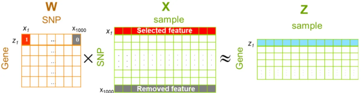
Figure 1.1: An example dataset in eQTL mapping
the activity of thousands of genes at once. The gene expression levels can be represented by continuous variables. Figure 1.1 shows an example dataset consisting of 1000 SNPs
{x1, x2,· · · , x1000}and a gene expression levelz1 for 12 individuals.
1.1 eQTL Mapping
For a QTL analysis, if the phenotype to be analyzed is the gene expression level data, then the analysis is referred to as the expression quantitative trait loci (eQTL) mapping. It aims to identify SNPs that influence the expression level of genes. It has been widely applied to dissect the genetic basis of gene expression and molecular mechanisms underlying complex traits (Bochner, 2003; Rockman and Kruglyak, 2006; Michaelson et al., 2009a). More formally, let X={xd|1≤d≤D} ∈RK×D be the SNP matrix denoting genotypes ofK SNPs ofD individuals andZ={zd|1≤d≤D} ∈RN×D be the gene expression matrix denoting
phenotypes ofN gene expression levels of the same set ofDindividuals. Each column ofXand Zstands for one individual. The goal of eQTL mapping is to find SNPs inX, that are highly associated with genes inZ.
regression coefficientsWusingℓ1 penalty. The objective function of Lasso is
min
W
1
2||Z−WX||
2
F+η||W||1 (1.1)
where|| · ||F denotes the Frobenius norm,|| · ||1 is theℓ1-norm. ηis the empirical parameter for theℓ1penalty. Wis the parameter (also called weight) matrix setting the limits for the space of linear functions mapping fromXtoZ. Each element ofWis the effect size of corresponding SNP and expression level. Lasso uses the least squares method withℓ1penalty. ℓ1-norm sets many non-significant elements ofWto be exactly zero, since many SNPs have no associations to a given gene. Lasso works even when the number of SNPs is significantly larger than the sample size (K ≫D) under the sparsity assumption.
(a) Strong association (b) No association
Figure 1.2: Examples of associations between a gene expression level and two different SNPs
Figure 1.3: Association weights estimated by Lasso on the example data
1.2 Group-Wise eQTL Mapping and Challenges
In a typical eQTL study, the association between each expression trait and each SNP is assessed separately (Cheung et al., 2005; Zhu et al., 2008; Tibshirani, 1996). This approach does not consider the interactions among SNPs and among genes. However, multiple SNPs may jointly influence the phenotypes (Lander, 2011), and genes in the same biological pathway are often co-regulated and may share a common genetic basis (Musani et al., 2007b; Pujana et al., 2007).
To better elucidate the genetic basis of gene expression, it is highly desirable to develop efficient methods that can automatically infer associations between a group of SNPs and a group of genes. We refer to the process of identifying such associations asgroup-wiseeQTL mapping. In contrast, we refer to those associations between individual SNPs and individual genes as
individualeQTL mapping. An example is shown in Figure 1.4. Note that an ideal model should allow overlaps between SNP sets and between gene sets; that is, a SNP or gene may participate in multiple individual and group-wise associations. This is because genes and the SNPs influencing them may play different roles in multiple biological pathways (Lander, 2011).
Besides, advanced bio-techniques are generating a large volume of heterogeneous datasets, such as protein-protein interaction (PPI) networks (Asur et al., 2007), and genetic interaction networks (Cordell, 2009). These datasets describe the partial relationships between SNPs and relationships between genes. Because SNPs and genes are not independent of each other, and there exist group-wise associations, the integration of these multi-domain
SNPs Genes
Group-wise association
Individual association
Figure 1.4: An illustration of individual and group-wise associations.
knowledge can be integrated. In literature, several methods based on Lasso have been proposed (Biganzoli et al., 2006; Kim and Xing, 2012; Lee and Xing, 2012; Lee et al., 2010) to leverage the network prior knowledge (Biganzoli et al., 2006; Kim and Xing, 2012; Lee et al., 2010; Lee and Xing, 2012; Jenatton et al., 2011). However, these methods suffer from poor quality or incompleteness of this prior knowledge.
In summary, there are several issues that greatly limit the applicability of current eQTL mapping approaches.
1. It is a crucial challenge to understandhow multiple, modestly-associated SNPs interact to influence the phenotypes(Lander, 2011). However, little prior work has studied the group-wise eQTL mapping problem.
2. The prior knowledge about the relationships between SNPs and between genes is often partial and usually includes noise.
3. Confounding factors such as expression heterogeneity may result in spurious associations and mask real signals (Michaelson et al., 2009b; Stegle et al., 2008; Gilad et al., 2008).
1.3 Thesis Statement
multi-domain heterogeneous data and can effectively detect group-wise associations for eQTL mapping.
1.4 Overview of the Developed Algorithms
This thesis proposes and studies the problem of group-wise eQTL mapping. We can decouple the problem into the following sub-problems.
• How can we detect group-wise eQTL associations with eQTL data only, i.e., with SNPs and gene expression profile data?
• How can we prepare more accurate prior knowledge about the relationships between SNPs and between genes by integrating multi-domain heterogeneous data?
• How can we incorporate the prior interaction structures between SNPs and between genes into eQTL mapping to improve the robustness of the model and the
interpretability of the results?
For the second sub-problem, this thesis presents a flexible and robust algorithm, CGC, to integrate heterogeneous graph data for clustering. Graphs (also called networks, but for the purpose of this thesis, we will maintain consistency by using the term “graphs”.) are widely used in representing relationships between instances, in which each node corresponds to an instance and each edge depicts the relationship between a pair of instances. Much prior knowledge about the relationships between SNPs and relationships between genes can be modeled as graphs. Biologists believe that a set of SNPs may play joint roles in a disease. Such interactions between SNPs can be modeled by a SNP interaction network. Even though the underlying biological processes are complex and only partially understood, it is well established that SNPs may alter the expression levels of related genes which may in turn have a cascading effect on other genes, e.g., in the same biological pathways (Michaelson et al., 2009c). The interactions between genes can be measured by correlations of gene expressions and represented by a gene interaction network. These two networks are heavily related because of the complicated relationships between SNPs and genes, as demonstrated in many expression quantitative trait loci (eQTL) studies (Lee and Xing, 2012). It is evident that a joint analysis becomes essential in these related domains. Multiple domain data, such as SNP-SNP interaction network, PPI network, and gene co-expression network, are able to provide more accurate prior knowledge about the grouping information of SNPs and genes. Data collected from different sources provide complimentary predictive powers, and combining their information can resolve ambiguity, thus helping to obtain a more accurate knowledge base. This thesis investigates the problem of clustering multiple heterogeneous data sets, where the cross-domain instance relationship is “many-to-many”. This problem has a wide range of applications and poses new technical challenges that cannot be directly tackled by traditional “multi-view” graph clustering methods (Kumar et al., 2011; Chaudhuri et al., 2009; Kumar and III, 2011). Based on the clustering consensus for different domains, we developed a robust and flexible approach that can incorporate multiple sources to enhance graph clustering performance. The proposed approach is robust even when the
users with the extent to which the cross-domain instance relationship violates the in-domain clustering structure, and thus enables users to re-evaluate the consistency of the relationship. The thesis further studies the trustworthiness of multi-source data, and extends the approach to enable it to automatically identify noisy domains and assign smaller weights to them for integration.
To address the third sub-problem, this thesis presents an algorithm, Graph-regularized Dual Lasso (GDL), to simultaneously learn the association between SNPs and genes and refine the prior networks. Traditional sparse regression problems in data mining and machine learning consider both predictor variables and response variables individually, such as sparse feature selection using Lasso. In the eQTL mapping application, both predictor variables and response variables are not independent of each other, and we may be interested in the joint effects of multiple predictors to a group of response variables. In some cases, we may have partial prior knowledge, such as the correlation structures between predictors, and correlation structures between response variables. This thesis shows how prior graph information would help improve eQTL mapping accuracy and how refinement of prior knowledge would further improve the mapping accuracy. In addition, other different types of prior knowledge,e.g., location information of SNPs and genes, as well as pathway information, can also be integrated for the graph
refinement.
1.5 Thesis Outline
The thesis is organized as follows:
• The algorithms to detect group-wise eQTL associations with eQTL data only (SET-eQTL, etc.) are presented in Chapter 2.
• The algorithm (CGC) to integrate heterogenous graph data for clustering is presented in Chapter 3.
CHAPTER 2: GROUP-WISE EQTL MAPPING
2.1 Introduction
A biological pathway is a series of actions among molecules in a cell that leads to a certain product or a change in a cell. For example, a pathway can trigger the assembly of new molecules, such as a fat or protein. Pathways play a key role in advanced studies of Genomics. In genetics, genes in the same biological pathway are often co-regulated and may share a common genetic basis (Musani et al., 2007b; Pujana et al., 2007). Consequently, it is crucial to understand how multiple modestly associated SNPs interact to influence the phenotypes (Lander, 2011). To address this issue, several approaches have been proposed to study the joint effect of multiple SNPs by testing the association between a set of SNPs and a gene expression trait. A
straightforward approach is to follow the gene set enrichment analysis (GESA) (Holden et al., 2008). Wu et al. proposed variance component models for SNP set testing (Wu et al., 2011). Aggregation-based approaches such as collapsing SNPs are investigated (Braun and Buetow, 2011). Listgarten et al. took confounding factors into consideration (Listgarten et al., 2013).
Despite their successes, these methods have two common limitations. First, they only study the association between a set of SNPs and a single expression trait, thus overlooking the joint effect of a set of SNPs on the activities of a set of genes, which may act and interact with each other to achieve certain biological function. Second, the SNP sets used in these methods are usually taken from known pathways. However, the existing knowledge on biological pathways is far from being complete. These methods cannot identify unknown associations between SNP sets or gene sets.
correlations between SNP sets and gene sets. However, this method needs the progeny strain information, which is used as a bridge for modeling the eQTL association graphs. A
two-graph-guided multi-task Lasso approach was developed in (Chen et al., 2012). This method needs to calculate gene co-expression network and SNP correlation network first. Errors and noises in these two networks may introduce bias in the final results. Note that all these methods do not consider confounding factors.
To better elucidate the genetic basis of gene expression and understand the underlying biology pathways, it is desirable to develop methods that can automatically infer associations between a group of SNPs and a group of genes. We refer to the process of identifying such associations asgroup-wiseeQTL mapping. In contrast, we refer to the process of identifying associations between individual SNPs and genes asindividualeQTL mapping. In this chapter, we propose several algorithms to detect group-wise associations. The first algorithm, SET-eQTL, makes use of a three-layer sparse linear-Gaussian model. It is able to identify novel associations between sets of SNPs and sets of genes. The results could provide new insights on how genes act and coordinate with each other to achieve certain biological functions. We further propose a fast and robust approach that is able to consider confounding factors and decoupleindividual
associations andgroup-wiseassociations for eQTL mapping. The model is a multi-layer
linear-Gaussian model and uses two different types of hidden variables: one capturing group-wise associations and the other capturing confounding factors (Gao et al., 2013; Leek and Storey, 2007; Joo et al., 2014; Fusi et al., 2012; Listgarten et al., 2013; Carlos M. Carvalhoa and West, 2008). We apply anℓ1-norm on the parameters (Lee et al., 2009; Tibshirani, 1996), which yields a sparse network with a large number of association weights being zero (Ng, 2004). We develop an efficient optimization procedure that makes this approach suitable for large-scale studies.
2.2 Related Work
Recently, various analytic methods have been developed to address the limitations of the traditional single-locus approach. Epistasis detection methods aim to find the interaction between SNP-pairs (Hoh and Ott, 2003; Hirschhorn and Daly, 2005; Balding, 2006; Musani et al., 2007a). The computational burden of epistasis detection is usually very high due to the large number of interactions that need to be examined (Nelson et al., 2001; Ritchie et al., 2001). Filtering-based approaches (Evans et al., 2006; Hoh et al., 2000; Yang et al., 2009), which reduce the search space by selecting a small subset of SNPs for interaction study, may miss important interactions in the SNPs that have been filtered out.
Statistical graphical models and Lasso-based methods (Tibshirani, 1996) have been applied to eQTL study. A tree-guided group lasso has been proposed in (Kim and Xing, 2012). This method directly combines statistical strength across multiple related genes in gene
expression data to identify SNPs with pleiotropic effects by leveraging the hierarchical clustering tree over genes. Bayesian methods have also been developed (Leopold Parts1, 2011; Stegle et al., 2010). Confounding factors may greatly affect the results of the eQTL study. To model
confounders, a two-step approach can be applied (Stegle et al., 2010; Jeffrey T. Leek, 2007). These methods first learn the confounders that may exhibit broad effects to the gene expression traits. The learned confounders are then used as covariates in the subsequent analysis. Statistical models that incorporate confounders have been proposed (Nicolo Fusi and Lawrence, 2012). However, none of these methods are specifically designed to find novel associations between SNP sets and gene sets.
limited to the priori knowledge on the predefined gene sets/pathways. On the other hand, the current knowledgebase on the biological pathways is still far from being complete.
A method is proposed to identify eQTL association cliques that expose the hidden structure of genotype and expression data (Huang et al., 2009b). By using the cliques identified, this method can filter out SNP-gene pairs that are unlikely to have significant associations. It models the SNP, progeny and gene expression data as an eQTL association graph, and thus depends on the availability of the progeny strain data as a bridge for modeling the eQTL association graph.
2.3 The Problem
Symbols Description
K number of SNPs
N number of genes
D number of samples
M number of group-wise associations
H number of confounding factors
x random variables ofKSNPs
z random variables ofNgenes
y latent variables to model group-wise associaiton
X∈RK×H SNP matrix data
Z∈RN×H gene expression matrix data
A∈RM×K group-wise association coefficient matrix betweenxandy
B∈RN×M group-wise association coefficient matrix betweenyandz
C∈RN×K individual association coefficient matrix betweenxandy P∈RN×H coefficient matrix of confounding factors
λ, γ regularization parameters
Table 2.1: Summary of Notations
Important notations used in this chapter are listed in Table 2.1. Throughout the chapter, we assume that, for each sample, the SNPs and genes are represented by column vectors. Let x= [x1, x2, . . . , xK]T represent theK SNPs in the study, wherexi ∈ {0,1,2}is a random variable corresponding to thei-th SNP. For example, 0, 1, 2 may encode the homozygous major allele, heterozygous allele, and homozygous minor allele, respectively. Letz= [z1, z2, . . . , zN]T represent theN genes in the study, wherezj is a continuous random variable corresponding to the
The traditional linear regression model for association mapping betweenxandzis
z=Wx+µ+ϵ, (2.1)
wherezis a linear function ofxwith coefficient matrixW. µis anN ×1translation factor vector.ϵis the additive noise of Gaussian distribution with zero-mean and varianceψI, whereψ
is a scalar. That is,ϵ∼N(0, ψI).
The question now is how to define an appropriate objective function to decomposeW which (1) can effectively detect both individual and group-wise eQTL associations, and (2) is efficient to compute so that it is suitable for large-scale studies. In the next, we will propose a group-wise eQTL detection method first, and then improve it to capture both individual and group-wise associations. Finally, we will discuss how to boost the computational efficiency.
2.4 Detecting Group-Wise Associations
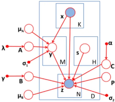
2.4.1 SET-eQTL Model
To infer associations between SNP sets and gene sets, we propose a graphical model as shown in Figure 2.3, which is able to capture any potential confounding factors in a natural way. This model is a two-layer linear Gaussian model. The hidden variables in the middle layer are used to capture the group-wise association between SNP sets and gene sets. These latent variables are presented asy= [y1, y2, . . . , yM]T, whereM is the total number of latent variables bridging SNP sets and gene sets. Each hidden variable may represent a latent factor regulating a set of genes, and its associated genes may correspond to a set of genes in the same pathway or participating in certain biological function. Note that this model allows a SNP or gene to
participate in multiple (SNP set, gene set) pairs. This is reasonable because SNPs and genes may play different roles in multiple biology pathways. Since the model bridges SNP sets and gene sets, we refer this method as SET-eQTL.
D N K
A
z B
µA
µB
1
2
K
x
y
M
Figure 2.1: The proposed graphical model with hidden variables
Figure 2.2: An example of the inferred sparse graphical model
resulting graphical model. There are two types of hidden variables. One type consists of hidden variables with zero in-degree (i.e., no connections with the SNPs). These hidden variables correspond to the confounding factors. Other types of hidden variables serve as bridges
connecting SNP sets and gene sets. In Figure 2.2,ykis a hidden variable modeling confounding effects.yiandyj are bridge nodes connecting the SNPs and genes associated with them. Note that this model allows overlaps between different (SNP set, gene set) pairs. It is reasonable because SNPs and genes may play multiple roles in different biology pathways.
2.4.2 Objective Function
From the probability theory, we have that the joint probability ofxandzis
p(x,z) =
∫
y
From the factorization properties of the joint distribution for a directed graphical model, we have
p(x,y,z) =p(y|x)p(z|y)p(x). (2.3)
Thus, we have
p(z|x) = p(x,z)
p(x) =
∫
y
p(y|x)p(z|y)dy. (2.4)
We assume that the two conditional probabilities follow normal distributions:
y|x∼ N(y|Ax+µA, σ21IM),
and
z|y∼ N(z|By+µB, σ22IN),
whereA∈RM×K is the coefficient matrix betweenxandy,B∈RN×M is the coefficient matrix betweenyandz. µA∈RM×1 andµB ∈RN×1are the translation factor vectors, of whichσ21IM andσ2
2IN are their variances respectively (σ1 andσ2 are constant scalars andIM andIN are identity matrices).
To impose sparsity, we assume that entries ofAandBfollow Laplace distributions:
A∼Laplace(0,1/λ),
and
B∼Laplace(0,1/γ).
β· N(y|µy,Σy) = N(y|Ax+µA, σ12IM)· N(z|By+µB, σ22IN) (2.5)
whereβis a scalar,µyandΣyare the mean and variance of a new normal distribution
respectively.
From Equations 2.4 and 2.5, we have that
p(z|x) =
∫
y
β· N(y|µy,Σy)dy=β (2.6)
Thus, maximizingp(z|x)is equivalent to maximizingβ. Next, we show the derivation ofβ. We first derive the value ofµy andΣ−y1 by comparing the exponential terms on both sides of
Equation 2.5.
N(y|Ax+µA, σ21IM)· N(z|By+µB, σ22IN)
= 1
(2π)M+N2 σM 1 σN2
exp{−12[σ12
1(y−Ax−µA)
T(y−Ax−µ
A)
+σ12 2
(z−By−µB)T(z−By−µB)]}
(2.7)
The exponential term in Equation 2.7 can be expanded as
Ψ=−12[σ12 1
(y−Ax−µA)T(y−Ax)
+σ2
2(z−By−µB)T(z−By)]
=−12[σ12 1
(yTy−yTAx−yTµ
A−xTATy+xTATAx
+xTATµ
A−µTAy+µTAAX+µTAµA) + σ12 2
(zTz−zTBy
−zTµB−yTBTz+yTBTBy+yTBTµB−µTBz+µ
T
BBy
+µTBµB)]
=−12[yT(σ12 1IM +
1 σ2
2B
T
B)y− σ22 1(x
TAT
y+µTAy)
− 2
σ2 2
(zTBy−µT
BBy) + σ12 1
(xTAT
Ax+ 2µT
AAx+µTAµA)
+σ12 2
(zTz−2µT
Bz+µTBµB)]
Thus, by comparing the exponential terms on both sides of Equation 2.5, we get
Σ−y1 = 1
σ2 1
IM +
1
σ2 2
BTB, (2.9)
µTyΣ−y1 = 1
σ2 1
(xTAT+µTA) + 1
σ2 2
(zTB−µTBB). (2.10)
Further, we have
µy=Σy[
1
σ2 1
(Ax+µA) +
1
σ2 2
(BTz−BTµB)]. (2.11)
WithΣ−1
y andµy, we can derive the explicit form ofβeasily by settingy=0, which
leads to the equation below:
β· 1
(2π)M2|Σy|
1 2
exp{−12µT
yΣ−y1µy}
= 1
(2π)M+N2 σM 1 σN2
exp{Ψy=0},
(2.12)
whereΨy=0 is the value ofΨwheny=0, and thereby
Ψy=0 =−12[σ12 1
(xTAT
Ax+ 2µT
AAx+µTAµA)
+σ12 2
(zTz−2µT
Bz+µTBµB)]
(2.13)
Thus, we get the explicit form ofβas
β= |Σy|
1 2
(2π)N2 σM 1 σN2
exp{Ψy=0+12(µTyΣ−y1µy)}. (2.14)
log-likelihood ofβd. Thus, our loss function is
J = −log∏Dd=1p(zd|xd)
= −∑Dd=1logp(zd|xd)
= −∑Dd=1logβd
(2.15)
Substituting Equation 2.14 into Equation 2.15, the expanded form of the loss function is
J(A,B,µA,µB, σ1, σ2)
= D2·N ln(2π) +D·Mln(σ1) +D·Nln(σ2) + D2 ln|Σ−y1|
+1
2
∑D
d=1{ 1 σ2
1
(xT
dA T
Axd+ 2µTAAxd+µTAµA)
+σ12 2
(zT
dzd−2µTBzd+µTBµB)−[σ12 1
(xT
dA
T+µT A)
+σ12 2
(zT
dB−µTBB)]Σy[σ12 1
(Axd+µA) + σ12
2
(BTzd−BTµB)]}
(2.16)
Taking into account the prior distributions ofAandB, we have that
p(z,A,B|x,µA,µB, σ1, σ2)
=β·Laplace(A|0,1/λ)·Laplace(B|0,1/γ)
(2.17)
Thus, we can have theℓ1-regularized objective function
max
A,B,µA,µB,σ1,σ2
log
D
∏
d=1
p(zd,A,B|xd,µA,µB, σ1, σ2),
which is identical to
min
A,B,µA,µB,σ1,σ2
[J +D·(λ||A||1+γ||B||1)], (2.18)
where|| · ||1 is theℓ1-norm. λandγ are theprecisionof the prior Laplace distributions ofAandB respectively, serving as the regularization parameters which can be determined by cross or
The gradient of the loss functionJ with respect toA,B,µA,µB,σ1, andσ2 are:
∇AJ =∑Dd=1(σ12 1Axdx
T d − σ14
1ΣyAxdx
T d − σ21
1σ22ΣyB
T zdxTd
+σ12 1µAx
T d − σ14
1ΣyµAx
T d +σ21
1σ22ΣyB
T
µBxTd)
(2.19)
∇BJ = σD2 2
BΣy+ σ14 2
(σ12 2
BΣyBT−IN)
∑D
d=1[(zd−µB) ·(zd−µB)T]BΣy+σ21
1σ42
∑D
d=1{BΣy[(Axd+µA)(zd−µB)TB
+BT(zd−µB)(Axd+µA)T]Σy−σ22(zd−µB)(Axd+µA)TΣy}
+σ41
1σ22BΣy
∑D
d=1[(Axd+µA)(xTdA T
+µTA)]Σy
(2.20)
∇µAJ =
1 2 ∑D d=1[ 2 σ2 1
(Axd+µA)− σ24
1
Σy(µA+Axd)− σ22 1σ22
Σy(BTzd−BTµB)] (2.21)
∇µBJ =
1 2 ∑D d=1[ 2 σ2 1
(−zd+µB) + σ24
1B
ΣyBT(zd−µB) + σ22 1σ22B
Σy(Axd+µA)] (2.22)
∇σ1J =
D·M σ1 −
D·tr(Σy)
σ3
1 +
∑D
d=1[−
xT
dATAxd+2µATAxd+µTAµA
σ3 1
+2(xTdAT+µTA)Σy(Axd+µA)
σ5
1 −
(xT dA
T+µT
A)Σ
2
y(Axd+µA)
σ7 1
+2(xTdA T+µT
A)Σy(BTzd−BTµB)
σ3
1σ22 −
2(xT dA
T+µT
A)Σ
2
y(BTzd−BTµB)
σ5 1σ22 −(zT
dB−µTBB)Σ2y(BTzd−BTµB)
σ3 1σ24
]
(2.23)
∇σ2J =
D·N σ2 −
D·tr(ΣyBTB)
σ3 2
+∑Dd=1[−zTdzd−2µTBzd+µTBµB
σ3 2
+2(zTdB−µ T
BB)Σy(B
Tz
d−BTµB)
σ5
2 −
(zT dB−µ
T
BB)ΣyB
TBΣ
y(BTzd−BTµB)
σ7 2
+2(zTdB−µ T
BB)Σy(Axd+µA)
σ2
1σ32 −
2(zT dB−µ
T
BB)ΣyB
TBΣ
y(Axd+µA)
σ2 1σ25 −(xT
dAT+µTA)ΣyB
TBΣ
y(Axd+µA)
σ4
1σ23 ]
2.5 Considering Confounding Factors
To infer associations between SNP sets and gene sets while taking into consideration confounding factors, we further propose a graphical model as shown in Figure 2.3. Different from the previous model, a new type of hidden variable,s= [s1, s2, . . . , sH]T, is used to model
confounding factors. For simplicity, we refer to this model asModel 1. The objective function of this model can be derivated using similar strategy as SET-eQTL.
Figure 2.3: Graphical model with two types of hidden variables
2.6 Incorporating Individual Effect
Figure 2.4: Refined graphical model to capture both individual and group-wise associations.
2.6.1 Objective Function
Next, we give the derivation of the objective function for the model in Figure 2.4. We assume that the two conditional probabilities follow normal distributions:
y|x∼N(y|Ax+µA, σ12IM), (2.25)
and
z|y,x∼N(z|By+Cx+Ps+µB, σ22IN), (2.26)
whereA∈RM×K is the coefficient matrix betweenxandy,B∈RN×M is the coefficient matrix betweenyandz,C∈RN×K is the coefficient matrix betweenxandzto capture the individual associations,P∈RN×H is the coefficient matrix of confounding factors.µA∈RM×1and
µB∈RN×1are the translation factor vectors,σ12IM andσ22IN are the variances of the two conditional probabilities respectively (σ1andσ2are constant scalars andIM andIN are identity matrices).
Since the expression level of a gene is usually affected by a small fraction of SNPs, we impose sparsity onA,BandC. We assume that the entries of these matrices follow Laplace distributions: Ai,j ∼Laplace(0,1/λ),Bi,j ∼Laplace(0,1/γ),andCi,j ∼Laplace(0,1/α). λ,γ andαwill be used as parameters in the objective function. The probability density function of
Thus, we have
y=Ax+µA+ϵ1, (2.27)
z=By+Cx+Ps+µB +ϵ2, (2.28)
whereϵ1 ∼N(0, σ12IM),ϵ2 ∼N(0, σ22IN). From Eq. (2.25) we have
By|x∼N(BAx+BµA, σ12BB T
), (2.29)
Assuming that the confounding factors follow normal distribution (Listgarten et al., 2013), s∼N(0,IH), then we have
Ps∼N(0,PPT). (2.30)
We substitute Eq. (2.29), (2.30) into Eq. (2.28), and get
z|x∼N(BAx+BµA+Cx+µB, σ12BB
T+PPT+σ2 2IN).
From the formula above, we observe that the summandBµAcan also be integrated inµB.
Thus to simplify the model, we setµA =0and obtain
z|x∼N(BAx+Cx+µB, σ21BB
T+PPT+σ2 2IN).
the negative log-likelihood (loss function) is
J =
D
∑
d=1
Jd
=−1·log
D
∏
d=1
p(zd|xd)
=
D
∑
d=1
(−1)·logp(zd|xd)
=D·N
2 log(2π) +
D
2 log|Σ|+ 1 2
D
∑
d=1
[(zd−µd)TΣ−1(zd−µd)],
(2.31)
where
µd=BAxd+Cxd+µB,
Σ=σ12BBT+WWT+σ22IN.
Moreover, taking into account the prior distributions ofA,BandC, we have p(zd,A,B,C|xd,P, σ1, σ2) =
exp(−Jd)·λ2
∏
i,jexp(−λ|Ai,j|)· γ2
∏
i,jexp(−γ|Bi,j|)·α2
∏
i,jexp(−α|Ci,j|).
(2.32)
Thus, we have theℓ1-regularized objective function
max
A,B,C,P,σ1,σ2
log
D
∏
d=1
p(zd,A,B,C|xd,P, σ1, σ2),
which is identical to
min
A,B,C,P,σ1,σ2
[J +D·(λ||A||1+γ||B||1+α||C||1)], (2.33)
where|| · ||1 is theℓ1-norm. λ,γ andαare theprecisionof the prior Laplace distributions ofA,B, andCrespectively. They serve as the regularization parameters and can be determined by cross or holdout validation.
The explicit expression ofµBcan be derived as follows. WhenA,B, andCare fixed, we
have
J = D2·N log(2π)+D2 log|Σ|+12∑Dd=1[(zd−BAxd−Cxd−µB)TΣ−1(zd−BAxd−Cxd−µB)].
µB =zd−BAxd−Cxd. WhenD >1, leveraging the fact thatΣ−1 is symmetric, we convert the problem into a least-square problem, which leads to
µB =
1
D
D
∑
d=1
(zd−BAxd−Cxd).
Substituting it into Eq. (2.31), we have
J =D·N
2 log(2π) + D
2 log|Σ|+ 1 2
∑D
d=1{[(zd−¯z)
−(BA+C)(xd−x¯)]TΣ−1[(zd−z¯)−(BA+C)(xd−x¯)]},
(2.34)
where
¯
x= 1
D
D
∑
d=1
xd, ¯z= 1
D
D
∑
d=1 zd.
The gradient of the loss function, which (without detailed derivation) is given in the below. 1). Derivative with respect toσ1
∇σ1O= 2σ1 D
∑
d=1
{tr[Ψd]BBT}. (2.35)
2). Derivative with respect toσ2
∇σ2O= 2σ2 D
∑
d=1
{tr[Ψd]}. (2.36)
3). Derivative with respect toA
∇AO=−
D
∑
d=1
[BTΣ−1td(xd−x¯)T]. (2.37)
4). Derivative with respect toB
∇BO=Ξ1+Ξ2, (2.38)
where
Ξ1=− D
∑
d=1
[Σ−1td(xd−x¯)TAT], (2.39)
(Ξ2)ij =σ21 D
∑
d=1
{tr[Ψd(EijBT+BEji)]}. (2.40)
We speed up this calculation by exploiting sparsity ofEij andtr[·]. (The following equation usesEinstein summation conventionto better illustrate the idea.)
(Ξ2)ij =σ12 D
∑
d=1
{tr[Ψd(EijBT +BEji)]}
=σ12
D
∑
d=1
{tr[ΨdEijBT +ΨdBEji]}
=σ12 D
∑
d=1
{tr[(Ψd)kl(Eij)lm(BT)mn + (Ψd)kl(B)ml (Eji)mn]}
=σ12
D
∑
d=1
{(Ψd)kl(Eij)lm(B T)m
k + (Ψd)kl(B) l
m(Eji)mk }
=σ12
D
∑
d=1
{(Ψd)ki(B T)j
k+ (Ψd)il(B) l j}
=σ12
D ∑ d=1 { N ∑ k=1
[(Ψd)k,i(BT)j,k] + N
∑
l=1
[(Ψd)i,l(B)l,j]}
=σ12 D ∑ d=1 { N ∑ k=1
[(BT)j,k(Ψd)k,i] + N
∑
l=1
[(Ψd)i,l(B)l,j]}.
(2.41)
Therefore,
Ξ2=σ12 D
∑
d=1
[(BTΨd)T +ΨdB]
=σ12
D
∑
d=1
[ΨTdB+ΨdB]
= 2σ21
D
∑
d=1
ΨdB.
(2.42)
5). Derivative with respect toC
∇CO=−
D
∑
d=1
[Σ−1td(xd−x¯)T]. (2.43)
6). Derivative with respect toP
∇PO=
D
∑
d=1
{tr[Ψd(EijPT+PEji)]}= 2 D
∑
d=1
ΨdP. (2.44)
2.6.2 Increasing Computational Speed
are fixed by following a similar technique as discussed in (Kang et al., 2008). For other
parameters, we develop an efficient method for calculating the inverse of the covariance matrix which is the main bottleneck of the optimization process.
2.6.2.1 Updatingσ2
When all other parameters are fixed, using spectral decomposition on(σ2 1BB
T
+WWT),
we have
Σ= (σ12BBT+WWT) +σ22IN
= [U,V] diag(λ1+σ22, ..., λN−q+σ22,0, ...,0)[U,V] T
=Udiag(λ1+σ22, ..., λN−q+σ22)UT,
(2.45)
whereUis anN×(N −q)eigenvector matrix corresponding to the nonzero eigenvalues;Vis an
N ×qeigenvector matrix corresponding to the zero eigenvalues. A reasonable solution should have no zero eigenvalues inΣ, otherwise the loss function would be infinitely big. Therefore,
q= 0. Thus
Σ−1 =Udiag( 1
λ1+σ22
, ..., 1
λN +σ22
)UT.
LetUT(zd−BAxd−Cxd−µB) =: [ηd,1, ηd,2, ..., ηd,N]T. Then solvingσ2 is equivalent
to minimizing
l(σ22) =D·N
2 log(2π) +
D
2
N
∑
s=1
log(λs+σ22) +
1 2 D ∑ d=1 N ∑ s=1 η2 d,s
λs+σ22
, (2.46)
whose derivative is
l′(σ22) = D 2
N
∑
s=1
1
λs+σ22
− 1 2 D ∑ d=1 N ∑ s=1 η2 d,s
(λs+σ22)2
.
This is a 1-dimensional optimization problem that can be solved very efficiently.
2.6.2.2 Efficiently Inverting the Covariance Matrix
the overall performance. This is for computing the inverse of the covariance matrix
Σ=σ12BBT+PPT+σ22IN,
which is much more time-consuming than other matrix multiplication operations.
We devise an acceleration strategy that calculatesΣ−1using formula (2.47) in the following theorem. The complexity of computing the inverse reduces toO(M3+H3).
Theorem 1. GivenB∈RN×M,P∈RN×H, and
Σ=σ22IN +σ12BBT+PPT.
Then
Σ−1 =T−TPS−1PTT, (2.47)
where
S=IH +PTTP, (2.48)
T=σ−22(IN −σ21B(σ22IM +σ21BTB)−1BT). (2.49)
The proof of Theorem 1 is provided in the following.
2.6.2.3 Preparation for Derivatives ofOfor Model 2
For notational simplicity, we denote
td= (zd−¯z)−(BA+C)(xd−x¯),
Ψd=
1
2(Σ
−1−Σ−1t
2.6.2.4 Proof of Theorem 1
Before giving the formal proof for Theorem 1, we first introduce Lemma 1, which follows from the definition of matrix inverse.
Lemma 1. For allU∈RN×M, ifIM +UTUis invertible, then
(IN +UUT)−1 =IN −U(IM +UTU)−1UT.
Here we provide a more general proof, which can be modified to derive more involved cases.
Proof. We denote
Q=σ22IN +σ12BB T
, (2.50)
that is,
Σ=σ22IN +σ12BBT+PPT =Q+PPT. (2.51)
By Lemma 1, we have
Q−1 =T=σ−22(IN −σ21B(σ 2
2IM +σ21B
TB)−1BT).
Qis symmetric positive definite, hence its inverse,T, is symmetric positive definite. Since every symmetric positive definite matrix has exactly one symmetric positive definite square root, we can write
T=RR,
whereRis anN ×N symmetric positive definite matrix.
It is clear that,Q=T−1 = (RR)−1 =R−1R−1, which leads to RQR=RR−1R−1R=IN, and therefore
Note that the above and the following formulas follow the fact thatRis symmetric. Once again, by Lemma 1, we have
(RΣR)−1 =IN −RPS−1PTRT,
where
S=IH +PTRTRP=IH +PTTP.
Therefore,
Σ−1 =R(RΣR)−1R=RR−RRPS−1PTRTR,
and thus
Σ−1 =T−TPS−1PTT
2.7 Optimization
To optimize the objective function, there are many off-the-shelfℓ1-penalized optimization tools. We use the Orthant-Wise Limited-memory Quasi-Newton (OWL-QN) algorithm described in (Andrew and Gao, 2007). The OWL-QN algorithm minimizes functions of the form
f(w) = loss(w) +c||w||1,
2.8 Experimental Results
We apply our methods (SET-eQTL,M odel1, andM odel2) to both simulation datasets and yeast eQTL datasets (Rachel B. Brem and Kruglyak, 2005) to evaluate its performance. For comparison, we select several recent eQTL methods, including LORS (Yang et al., 2013), MTLasso2G (Chen et al., 2012), FaST-LMM (Listgarten et al., 2013) and Lasso (Tibshirani, 1996). The tuning parameters in the selected methods are learned using cross-validation. All experiments are performed on a PC with 2.20 GHz Intel i7 eight-core CPU and 8 GB memory.
2.8.1 Simulation Study
We first evaluate whether Model 2 can identify both individual and group-wise associations. We adopt a similar setup for simulation study to that in (Lee and Xing, 2012; Yang et al., 2013) and generate synthetic datasets as follows. 100 SNPs are randomly selected from the yeast eQTL dataset (Rachel B. Brem and Kruglyak, 2005).N gene expression profiles are generated byZj∗ =βj∗X+ Ξj∗+Ej∗ (1≤j ≤N), whereEj∗ ∼N(0, ηI)(η= 0.1) denotes Gaussian noise.Ξj∗is used to model non-genetic effects, which is drawn fromN(0, ρΛ), where
ρ= 0.1. Λis generated byFFT, whereF∈RD×U andF
ij ∼N(0,1). U is the number of hidden factors and is set to 10 by default. The association matrixβ is shown in the top-left plot in Figure 2.5. The association strength is 1 for all selected SNPs. There are four group-wise associations of different scales in total. The associations on the diagonal are used to represent individual
association signals incis-regulation.
The remaining three plots in Figure 2.5 show associations estimated byM odel2. From the figure, we can see thatM odel2well captures both individual and group-wise signals. For
comparison, Figure 2.6 visualizes the association weights estimated byM odel1andM odel2
when varying the number of hidden variables (M). We observe that forM odel1, whenM = 20, most of the individual association signals on the diagonal are not captured. AsM increases, more individual association signals are detected byM odel1. In contrast,M odel2recovers both
β (true)
20 40 60 80 100 20 40 60 80 100 0 0.2 0.4 0.6 0.8 1 Model2 C
20 40 60 80 100 20 40 60 80 100 0 0.2 0.4 0.6 0.8 1
Model2 B×A
20 40 60 80 100 20 40 60 80 100 0 0.2 0.4 0.6 0.8 1
Model2 B×A+C
20 40 60 80 100 20 40 60 80 100 0 0.2 0.4 0.6 0.8 1
Figure 2.5: Ground truth ofβand linkage weights estimated byM odel2on simulated data.
Model1 B×A (M=80)
20 40 60 80 100 20 40 60 80 100 0 0.2 0.4 0.6 0.8 1
Model1 B×A (M=40)
20 40 60 80 100 20
40
60
80
100
Model2 B×A+C (M=20)
20 40 60 80 100 20 40 60 80 100 0 0.2 0.4 0.6 0.8 1
Model2 B×A+C (M=40)
20 40 60 80 100 20 40 60 80 100 0 0.2 0.4 0.6 0.8 1
Model2 B×A+C (M=80)
20 40 60 80 100 20 40 60 80 100 0 0.2 0.4 0.6 0.8 1 0 0.2 0.4 0.6 0.8 1
Model1 B×A (M=20)
20 40 60 80 100 20 40 60 80 100 0 0.2 0.4 0.6 0.8 1
Figure 2.6: Association weights estimated byM odel1andM odel2.
Next, we generate 50 simulated datasets with different signal-to-noise ratios (defined as
SN R=
√
V ar(βX)
V ar(Ξ+E)) in the eQTL datasets (Yang et al., 2013) to compare the performance of the selected methods. Here, we fixH = 10, ρ= 0.1, and use differentη’s to controlSN R. For each setting, we report the average result from the 50 datasets. For the proposed methods, we use BA+Cas the overall associations. Since FaST-LMM needs extra information (e.g., the genetic similarities between individuals) and uses PLINK format, we do not list it here and will compare it on the real data set.
0 0.02 0.04 0.06 0.08 0.1 0 0.2 0.4 0.6 0.8 1 FPR TPR Model 2 Model 1 SET−eQTL MTLasso2G LORS Lasso
(a) ROC curve(SN R=1.16)
0 0.02 0.04 0.06 0.08 0.1 0 0.2 0.4 0.6 0.8 1 FPR TPR Model 2 Model 1 SET−eQTL MTLasso2G LORS Lasso
(b) ROC curve(SN R=0.13)
0 0.02 0.04 0.06 0.08 0.1 0 0.2 0.4 0.6 0.8 1 FPR TPR Model 2 Model 1 SET−eQTL MTLasso2G LORS Lasso
(c) ROC curve(SN R=0.08)
Figure 2.7: The ROC curve of FPR-TPR on simulated data.
Lasso LORS MTLasso2GSET−eQTL Model 1 Model 2 0 0.1 0.2 0.3 0.4 0.5 0.6 0.7 0.8 0.9 1
AUC of FPR−TPR curve
SNR=0.08 SNR=0.13 SNR=1.16
(a) AUC of FPR-TPR curve
Lasso LORS MTLasso2GSET−eQTL Model 1 Model 2 0 0.1 0.2 0.3 0.4 0.5 0.6 0.7 0.8 0.9 1
AUC of FPR−TPR curve
SNR=0.08 SNR=0.13 SNR=1.16
(b) AUC of precision-recall curve
Figure 2.8: The areas under the precision-recall/FPR-TPR curve (AUCs).
(AUCs) (Chen et al., 2012) are shown in Figure 2.8. It can be seen thatM odel2outperforms all alternative methods by a large margin.M odel2outperformsM odel1because it considers both group-wise and individual associations. M odel1outperforms SET-eQTL because it considers confounding factors that is not considered by SET-eQTL. SET-eQTL considers all associations as group-wise, thus it may miss some individual associations. MTLasso2G is comparable to LORS because MTLasso2G considers the group-wise associations while neglecting confounding factors. LORS considers the confounding factors, but does not distinguish individual and group-wise associations. LORS outperforms Lasso since confounding factors are not considered in Lasso.
2.8.1.1 Shrinkage ofCandB×A