LABOR MARKET ASSIMILATION OF IMMIGRANTS
Apoorva Jain
A dissertation submitted to the faculty of the University of North Carolina at Chapel Hill in partial fulfillment of the requirements for the degree of Doctor of Philosophy in the
Department of Computer Science.
Chapel Hill 2017
Approved by: Klara S. Peter Helen Tauchen Luca Flabbi
c
○2017 Apoorva Jain
ABSTRACT
Apoorva Jain: LABOR MARKET ASSIMILATION OF IMMIGRANTS. (Under the direction of Klara S. Peter)
The economic contribution of migrants to a host country are well known: they work in sectors where labor is scarce, create jobs when becoming entrepreneurs, and also contribute by paying taxes. For such potential contributions to materialize, immigrants’ successful par-ticipation in the labor market is crucial. This dissertation analyzes the process of immigrant assimilation in the host country’s labor market. The dissertation consists of two chapters, both of which use German Socio-economic Panel from 1984 to 2014. Germany’s long history of immigration and the availability of a long panel dataset makes the country a good choice for this study.
high quality counterparts. Third, immigrants who have a greater propensity to migrate early have a higher individual rate of assimilation.
ACKNOWLEDGMENTS
This dissertation would not have been possible without the help and efforts of many. First and foremost, I would like to thank my advisor, Klara S. Peter, for supporting my work, providing invaluable guidance, and encouraging my ideas. Her passion for economics is contagious. I am also extremely grateful to my committee members for their constructive feedback: Prof. Tauchen for helping me develop the theoretical foundations of my research; Prof. Flabbi for giving beneficial suggestions on improving the empirical strategy; Prof. Becker for his detailed feedback; and Prof. Gilleskie for improving my writing skills. I am also very thankful to Prof. Tiago Pires for long and thoughtful discussions about my research work.
TABLE OF CONTENTS
LIST OF TABLES . . . xi
LIST OF FIGURES . . . xii
1 Timing of Migration, Immigrant Quality and Labor Market Assimila-tion: Evidence from a Long Panel in Germany . . . 1
1.1 Introduction . . . 1
1.2 Theoretical Model of Timing of Migration . . . 6
1.3 Joint Model of Wage Assimilation and Timing of Migration . . . 10
1.3.1 Problem of Endogeneity in Length of Stay . . . 10
1.3.2 Timing of Migration . . . 13
1.3.3 Wage Assimilation . . . 14
1.3.4 Joint Estimation . . . 16
1.3.5 Selection into Employment . . . 21
1.4 Data and Variables . . . 22
1.4.1 Variables in Timing of Migration Equation . . . 24
1.4.2 Variables in Wage Assimilation Equation . . . 26
1.5 Model Estimates . . . 27
1.5.1 Reduced Form Estimates . . . 27
1.5.2 Joint Model Estimates . . . 30
1.6 Conclusion . . . 33
1.7 Tables . . . 35
2 Limits to Wage Growth: Understanding the Wage Divergence between
Immigrants and Natives (with Klara S. Peter) . . . 59
2.1 Introduction . . . 59
2.2 Empirical Evidence on the Economic Assimilation of Immigrants . . . 63
2.2.1 Sample composition . . . 63
2.2.2 Labor market outcomes of immigrants and natives . . . 64
2.2.3 Wage returns to the length of stay since migration . . . 65
2.2.4 Relative wage profiles: first evidence of wage divergence . . . 67
2.2.5 Selection into employment and survey participation . . . 69
2.3 Theoretical Model of Wage Convergence . . . 70
2.3.1 Set-up . . . 70
2.3.2 Immigrant wage growth . . . 73
2.3.3 Wage convergence/divergence between immigrants and natives . . . . 74
2.4 Empirical Strategy . . . 76
2.4.1 Empirical model of wage convergence between immigrants and natives 76 2.4.2 Measuring factors of wage convergence . . . 77
2.4.3 Selectivity bias and exclusion restrictions . . . 81
2.4.4 Endogeneity of post-migration investment in human capital . . . 84
2.5 Results . . . 86
2.5.1 Dependent variable . . . 86
2.5.2 Reduced form model of wage convergence . . . 87
2.5.3 Alternative Specifications . . . 90
2.5.4 Post-migration accumulation of human capital . . . 92
2.5.5 Channels of wage divergence . . . 93
2.7 Tables . . . 97
2.8 Figures . . . 106
A Appendices for Chapter 1 . . . 111
A.1 Data Appendix . . . 111
A.1.1 Construction of Linguistic Distance . . . 111
A.1.2 Description of Variables . . . 113
A.2 Technical Appendix . . . 118
A.2.1 Joint Estimation . . . 118
A.2.2 Modified Joint Likelihood Function . . . 119
A.2.3 Calculating the Range for Numerical Integration . . . 123
B Appendices for Chapter 2 . . . 125
B.1 Data Appendix . . . 125
B.1.1 Samples . . . 125
B.1.2 Weights . . . 126
B.2 Description of Variables . . . 128
B.2.1 Individual-Level Variables . . . 128
B.2.2 Home Country Characteristics . . . 134
B.3 Additional Estimates . . . 139
B.4 Comparative Statics . . . 141
B.5 Web Appendix . . . 143
LIST OF TABLES
1.1 Summary Statistics for Key Variables . . . 35
1.2 Key Variables in Timing of Migration and Wage Assimilation Equations . . 36
1.3 Timing of Migration: Reduced Form Estimates for Men . . . 37
1.4 Timing of Migration: Reduced Form Estimates for the Full Sample . . . 39
1.5 Probit Estimates for Selection in Employment . . . 41
1.6 Wage Assimilation Equation: Reduced Form Estimates for Men . . . 42
1.7 Wage Assimilation Equation: Reduced Form Estimates for the Full Sample . 43 1.8 Timing of Migration: Joint Model Estimates for Men . . . 44
1.9 Wage Assimilation: Joint Estimates for Men . . . 45
1.10 Variance-Covariance Structure of Immigrant Quality, Propensity of Early-Migration and Individual Variation from Average Rate of Assimilation: Joint Model Estimates for Men . . . 45
1.11 Timing of Migration: Joint Model Estimates for Full Sample . . . 46
1.12 Wage Assimilation: Joint Estimates for Full Sample . . . 47
1.13 Variance-Covariance Structure of Immigrant Quality, Propensity of Early-Migration and Individual Variation from Average Rate of Assimilation: Joint Model Estimates for Full Sample . . . 47
2.1 Sample Composition . . . 97
2.2 Labor Market Outcomes of Natives and Immigrants . . . 98
2.3 Summary Statistics . . . 98
2.4 Baseline Specification, Reduced Form . . . 100
2.5 Selection Probit Equation, Marginal Effects . . . 101
2.6 Alternative Specification I, Reduced Form . . . 102
A.1 Languages with Highest and Lowest Linguistic Distance from Standard Ger-man in SOEP . . . 112
LIST OF FIGURES
1.1 A Typical Immigrant’s Timeline . . . 17
1.2 Histogram of Age at Migration by Gender . . . 48
1.3 Age-Earnings Profile by Gender . . . 48
1.4 Non Parametric Estimates . . . 49
1.5 Non Parametric Estimates . . . 50
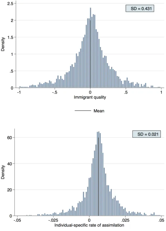
1.6 Distribution of Immigrant Quality and Individual-specific Rate of Assimila-tion: Men Only Specification . . . 51
1.7 Distribution of Propensity to Migrate Early: Men Only Specification . . . . 52
1.8 Correlation between Immigrant Quality, Individual-specific Rate of Assimila-tion, and Propensity to Migrate Early: Men Only Specification . . . 53
1.9 Correlation between Immigrant Quality, Individual-specific Rate of Assimila-tion, and Propensity to Migrate Early: Men Only Specification . . . 54
1.10 Distribution of Immigrant Quality and Individual-specific Rate of Assimila-tion: Full Sample Specification . . . 55
1.11 Distribution of Propensity to Migrate Early: Full Sample Specification . . . 56
1.12 Correlation between Immigrant Quality, Individual-specific Rate of Assimila-tion, and Propensity of Early Migration: Full Sample Specification . . . 57
1.13 Correlation between Immigrant Quality, Individual-specific Rate of Assimila-tion, and Propensity of Early Migration: Full Sample Specification . . . 58
2.1 Individual Returns to Years Since Migration . . . 106
2.2 Age-Wage Profiles . . . 107
2.3 Employment Outcomes and Survey Participation over Life Cycle . . . 108
2.4 Demand and Supply of Training Programs . . . 109
2.5 Year Effects and Secular Trend in Wage Convergence . . . 109
2.6 Perceived level of Discrimination . . . 110
Chapter 1: Timing of Migration, Immigrant Quality and Labor Market Assimilation: Evidence from a Long Panel in Germany
1.1 Introduction
The immigrant assimilation hypothesis (Chiswick,1978) conjectures that immigrants ac-quire host country-specific human capital, that this increases with time spent in the host country (henceforth called length of stay), and that they experience wage growth. The rate of wage growth with respect to years since migration is known as the rate of assimilation. Existing studies, such as Borjas (1987, 1994), Hu (2000) and Lubotsky (2007), which have assumed that years since migration is exogenous, have estimated an average rate of assimi-lation.1 The length of stay depends on the timing of migration and, thus, it is endogenously determined. This paper relaxes the exogeneity assumption by developing and estimating a joint model of the timing of migration and wage assimilation in the labor market. The joint model also measures individual-specific rates of assimilation. These individual specific rates can be used to better inform immigration policies, which until now were based solely on the quality of the immigrant at the time of migration and not her future ability to assimilate well.
Forward-looking individuals decide whether or not to migrate on the basis of the net expected utility of migration; in other words, the optimal timing of migration is a choice. Consequently, years since migration, which is age minus age at migration, is not exogenous. Ignoring the selective timing of migration can lead to an inconsistent estimate of the rate of assimilation. Moreover, the commonly estimated average rate of assimilation neglects the potential differences in the post-migration rate of human capital acquisition between 1Rarely, papers estimate assimilation rates for subgroups based on arrival cohorts such asBorjas(2013)
immigrants who migrated at different ages. According to the economic theory of human capital, younger individuals have a greater incentive to acquire human capital. Given that differences in human capital investment result in different rates of assimilation, a twenty year-old and a forty year-old immigrant are likely to have different rates of assimilation.
It is necessary to jointly estimate the timing of migration and wage assimilation to account for unobserved individual factors that affect both the timing of migration and the immigrants performance in the host country’s labor market. Unobserved characteristics, such as risk attitude, personality, and ability, can affect the propensity to migrate and earnings growth in the host country. For instance, immigrants with a high ability might have a lower cost of migration and, thus, a higher propensity to migrate early. High ability individuals are likely to experience high wage growth after migration.
In contrast, risk-averse individuals might have a low propensity to migrate early, and they might avoid risky yet profitable job opportunities in the host country. In other words, risk-averse immigrants might have a slower rate of assimilation. In such cases, the rate of assimilation is correlated with both an unobserved propensity to migrate and the timing of migration. To account for the interdependence of the timing of migration and wage assimilation, the two processes should be estimated jointly.
Most papers that estimate the wage assimilation equation, such as Borjas (1987, 1994, 1988) and Antecol et al. (2006), use census data to estimate an average rate of assimilation while controlling for arrival-cohort-specific unobserved immigrant quality.2 Thus, they as-sume that immigrants within an arrival cohort have similar unobserved characteristics. A few papers, including Fertig and Schurer (2007) and Cobb-Clark et al. (2012), use longitu-dinal data and individual fixed effects to account for time-constant individual unobserved heterogeneity. However, both longitudinal and cross-sectional studies implicitly assume that unobserved immigrant quality directly affects wage level but not through the returns to 2A few papers likeCobb-Clark(1993) account for unobserved immigrant quality using a control function
the length of stay - i.e., they assume that rate of assimilation does not vary with immi-grant quality.3 This paper relaxes these assumptions to estimate individual-specific rates of assimilation that vary with immigrant quality.
While wage assimilation estimates are common in the literature, few papers estimate the timing of the migration equation. The papers that do are limited by the fact that they focus on the effect of a single factor on out-migration and analyze either domestic migration or migration from a single country over a short period of time. For instance, Reed et al. (2010) examine gender differences in mobility in Ghana; Henry et al. (2004) analyze the effect of rainfall on first out-migration in Burkin Faso; Ezra and Kiros (2001) study the effect of drought on rural out-migration within Ethiopia; and Hare (1999) analyzes rural out-migration within China. In contrast, my study examines data on a much larger scale: I estimate variation in the timing of migration for immigrants from over 100 countries during a 53-year period (1961-2014).
To address these shortcomings in the existing models, I develop and estimate a joint model of wage assimilation and the timing of migration. The joint model links the two equations through correlation between immigrant quality, the individual-specific rate of assimilation (both of which appear in the wage assimilation equation), and the unobserved propensity to migrate early (which appears in the timing of migration equation). The timing of migration is modeled as a continuous time parametric proportional hazard in which the hazard of early migration depends on individual characteristics, macro-level factors of migration, and an unobserved individual propensity to migrate early. The wage assimilation equation is a linear mixed model in which the log of the wage depends on various individual-specific factors, including years since migration and unobserved immigrant quality. The individual-specific rate of assimilation is estimated using a random coefficient on years since migration variable. Using the parameters estimated in the joint model, I estimate the Best Linear 3Borjas(2013) andFertig and Schurer(2007) are notable exceptions which estimate rates of assimilation
Unbiased Predictions (BLUPs) which help recover the complete joint distribution of the individual-specific rate of assimilation, immigrant quality, and the propensity to migrate early. The joint distributions also help in understanding the relationship between these components.
However, the joint model estimation suffers from an unignorable limitation, the inability to include non-migrants in the study. As is the case with most migration studies, we only have information on immigrants within a host country. Existing papers such as Borjas (1985, 1994) Hu (2000) and Fertig and Schurer (2007) use migration cohort or individual fixed effects to account for self-selection of immigrants. In the same spirit, I account for permanent unobserved heterogeneity which should partly control for the issue of selection of immigrants.
I estimate the proposed joint model using data on immigrants in the German Socio-Economic Panel (henceforth called SOEP) for the period 1984-2014.4 Since the 1950s, Ger-many has had a long and diverse history of immigration, and for this reason it provides an excellent location to study immigrants economic assimilation. As of 2015, Germany has hosted more than 12 million immigrants, which is the second highest stock of immigrants (behind the United States of America) in the world. Moreover, SOEP over-samples immi-grants and provides information on the country of origin and the year of migration for a large sample of immigrants. Using this information, I construct pre-migration histories from which I estimate the timing of the migration equation. To explain pre-migration histories, I collect data on macro-level migration factors from 1961 to 2014, and these are then merged with individual level pre-migration characteristics using the year of migration and country of origin. These long panel data allow me to estimate long-term assimilation rates, which in the literature is a rare achievement.
The joint model is estimated for individuals who migrated after the age of 13 between 4 The data used in this paper were made available to us by the German Socio-Economic Panel Study at
1961 and 2014. I limit the sample to youth and adult migrants because: (1) child migrants are not likely to make individual migration decisions and (2) the assimilation experience of child migrants could differ from that of youth and adult migrants. For instance, Bleakley and Chin(2004,2008,2010) show that child migrants assimilate faster and better than adult migrants.
The model estimates reveal four key findings. First, the exogeneity assumption of years since migration results in an upward bias in the average rate of assimilation. After accounting for the selective timing of migration, the average rate of assimilation drops from 1 percent to 0.6 percent. Second, there is a remarkable degree of variation in the individual-specific rates of assimilation. They vary from negative 10 percent to 7.1 percent. Third, the estimates predict a strong negative correlation between the individual-specific rate of assimilation and immigrant quality. This finding suggests that relative to high quality immigrants, low quality immigrants invest more in human capital after migration and, consequently, they have a higher rate of assimilation. Thus, we observe a catch-up effect between low-quality and high-quality immigrants. These findings are consistent with the theoretical predictions of Duleep and Regets (1999) and Borjas (1999). The Immigrant Human Capital Investment (IHCI) model of Duleep and Regets (1999) predicts that immigrants who have less transferable skills would have a lower opportunity cost of acquiring human capital in the host country. Thus, immigrants with less transferable skills are more likely to invest in human capital after migration and, thus, they have a higher rate of assimilation. Also, the immigrant human capital accumulation theory of Borjas (1999) predicts a conditional convergence if there is “relative substitutability” between pre-migration human capital and post-migration human capital.
influences the propensity for early migration and, subsequently, the timing of migration. In either case, the timing of migration and wage assimilation are interdependent - a finding that validates the paper’s hypothesis and highlights the need to estimate these equations jointly. The rest of the paper is organized in five sections. Section1.2presents a simple theoretical model of the timing of migration that explains how individuals decide the optimum period of working life to spend in the host-country so as to maximize expected lifetime earnings. Section1.3illustrates the endogeneity problem in years since migration variable and develops the joint model of the timing of migration and wage assimilation. In Section1.4, I discuss the data and variables used to estimate the joint model. Section1.5 discusses model estimates. Finally, Section 1.6 concludes.
1.2 Theoretical Model of Timing of Migration
In this section, I present a simple model that explains how immigrants decide the time of migration (age at migration) which in turn determines the length of the working life spent in the host country. In the model, individuals decide the optimal time of migration that maximizes the net expected lifetime earnings. The migration event is assumed to be an absorbing state; that is, once the individual migrates to the host country, she does not out-migrate until the end of the working life.5
A related model was presented byZimmermann and Constant (2012) that illustrates the role of age in migration decisions. My model differs from their model in two major ways. First, I introduce the role of skill transferability in the migration decision. As skills are not perfectly transferable over international borders, individuals can only market a fraction of their pre-migration skills. The degree of skill-transferability is the fraction of pre-migration skills that are valuable in the host-country. The degree of skill transferability is allowed to vary by the age at migration, the time spent in the host country and other exogenous 5This assumption is only for simplification and can be relaxed. Please refer toDustmann and G¨orlach
factors. Thus, we gain insight into how differences in exogenous factors which affect the skill-transferability affect the marginal cost of migration and the optimum time of migration. Second, as the model involves maximization of lifetime earnings (and not utility), I only focus on working age individuals and working life period.
Model Set-up The individual begins working in the origin country at age ab which is
also the first time she decides whether to migrate or not. The working life spans from ab to
A. The individual works in the home country from ab till the time of migration am and in
the host country from am untilA. Thus, the total working life spent in the host country is
A−am. The average wage per unit of human capital H in the origin country is wo and in
the host country is wh. Wages in both origin and host country are a function of individual’s
age.
Individuals can only market a fraction of their pre-migration skills δH in the host coun-try’s labor market where 0 < δ ≤ 1. The degree of skill transferability δ varies with the age at migration am, the time in the host country a −am and other exogenous factors γ.
Country of origin, ethnicity and other exogenous factors captured by γ only contribute an additive shift in the degree of skill transferability and their effect does not change with the time of migration. Migration involves a one time cost C that varies by age at migration. For simplicity, it is also assumed that there is no accumulation of formal human capital post-migration.
The present value of net lifetime earnings for an individual who migrates at am and
discounts future earnings by ρ is given by the following expression:
E(am) = am
Z
ab
e−ρawo(a)Hda−C(am)e−ρam
+
A
Z
am
e−ρawh(a)δ(am, a−am, γ)Hda
(1.1)
The first term represents the discounted earnings in the origin country fromabtoam. The
second term is the one-time cost of migration at ageam and the third term is the discounted
earnings in the host country from am to A.
The optimal time of migration a∗m is given by equating the first derivative of Equation 1.1 with respect to am to zero:
E1(am) =e−ρawo(a)H+ρC(am)e−ρam −C0(am)e−ρam
−e−ρamwh(am)δ(am,0, γ)H+ A
Z
am
e−ρawh(a)(δ1−δ2)Hda = 06
(1.2)
where the left hand side gives the marginal benefit and the right hand side gives the marginal cost of migrating a year later. Rearranging Equation 1.2 yields the following expression:
e−ρawo(a)H+ρC(am)e−ρam −C0(am)e−ρam
=e−ρamwh(am)δ(am,0, γ)H− A
Z
am
e−ρawh(a)(δ1−δ2)Hda
(1.3)
The marginal benefit includes the discounted wage in the origin country for an additional year and the postponed cost of migration minus the change in cost of migration due to the delay. There are two reasons why we might expect the change in cost C0(am) to be negative
i.e. the cost of migration decreases with age at migration. First, selective immigration policies that favor high-skilled immigrants make it easier for older immigrants to obtain a work visa. Second, it might also be easier for older individuals to collect information about migration process and job opportunities in the host country. Under such cases, delaying migration would increase the marginal benefit from reduced cost of migration a year later.
The marginal cost includes the lost earnings in the host country at arrival (i.e. when years since migration is zero) minus the change in the future stream of earnings in the host country due to migrating a year later. It is assumed that δ1 < 0 i.e. the degree of skill
6δ
transferability decreases with an increase in age at migration and δ2 > 0 i.e. the degree of skill transferability increases with time spent in the host country. Thus, with increase in age at migration, the change in future stream of earnings in the host country decreases and the marginal cost increases.
There is substantial evidence that suggestsδ1is negative. For instance,Bleakley and Chin (2004, 2008, 2010) show that younger aged migrants are more proficient in host-country’s language, thus they perform better in the host-country’s labor market and are more socially assimilated than their older counterparts.7 Similarly, Immigrant Assimilation Hypothesis suggests that δ2 is positive. Duleep and Regets(1999) show that degree of skill transferabil-ity increases with the investment in host-country specific human capital. As investment in human capital post-migration depends on the time spent in the host country, skill transfer-ability is expected to increase with time in the host country.
According to Equation 1.3, the optimal age at migrationa∗m is chosen when the marginal benefit equals the marginal cost of migrating. Migration does not occur if the marginal benefit from delaying migration is always higher than the marginal cost. On the other hand, if the marginal cost is always higher than the marginal benefit, the individual would choose to migrate at the beginning of working lifeab. The existence of an interior solution depends
on the discounting factor, the magnitude of wage loss due to skill transferability and the change in the cost of migration from postponed migration.
Exogenous factors of skill transferability would also affect the optimal time of migration through differences in earnings at arrival. Let γ capture cultural and linguistic similarity between the origin and host country. Thus, the degree of skill transferability increases with an in increase in γ, i.e.,δγ >0. To understand the effect ofγ ona∗m, we take a derivative of
Equation 1.3 with respect to γ:
7They also asserted that these findings support Critical Period Hypothesis of language acquisition.
E11(a∗m(γ), γ)
∂a∗m
∂γ +E1γ(a ∗
m(γ), γ) = 0 (1.4)
where
E1γ(a∗m(γ), γ) = −e
−ρamw
h(am)δγH (1.5)
As E11<0, E1γ <0 and δγ =α , this implies
∂a∗m
∂γ <0 (1.6)
Thus, the model predicts that migrants from countries similar to the host country would migrate at an earlier age.
From the theoretical model, it is clear that the time of migration is not randomly assigned and hence years since migration in the host country is also not exogenous. In the next section, I illustrate how the failure to account for selective timing of migration can lead to an inconsistent estimate of the rate of wage assimilation.
1.3 Joint Model of Wage Assimilation and Timing of Migration
This section first discusses the implicit assumptions made when years since migration is treated as an exogenous variable. Next, it develops a joint model of the timing of migration and wage assimilation that relaxes these assumptions. The joint model also accounts for selection into non-employment using inverse propensity weighting.
1.3.1 Problem of Endogeneity in Length of Stay
A typical empirical model of the economic assimilation of immigrants (refer to Chiswick (1978),Borjas (1985, 1987) and Duleep and Regets (2002)) is estimated using the following wage equation:
whereWis is the log of wage of individuali at times,Xis is a vector of immigrant’s observed
characteristics in the host country that often includes age (or experience) and education, Y SMis is years since migration (or length of stay) calculated as the difference between the
year of survey and the year of migration (Ys−Ym), φ(s) is a linear time trend capturing the
business cycle and Ci captures time-constant cohort-specific unobserved heterogeneity. A
few panel studies likeFertig and Schurer (2007) sometimes include time-constant individual heterogeneity αi instead of Ci.
δ is the average wage return on spending a year in the host country instead of origin country. Thus, δ represents the rate of assimilation where assimilation is defined in a way similar to LaLonde and Topel (1992): “assimilation occurs, if between two observationally equivalent persons, the one with greater time in the United States typically earns more”. Thus, the base group is the immigrant herself and a positive value ofδ indicates assimilation within the immigrant group rather than with respect to their native counter-parts. In this paper, I follow a similar definition of assimilation but estimate an individual-specific rate of assimilation and not just the average.8 I discuss the estimation of individual-specific rate of assimilation in Section 1.3.3.
Previous studies have treated Y SMis as exogenous. However, there are several reasons
why this leads to biased estimates. To understand them, let us consider an individual’s migration decisionMi(a) at agea:
Mi(a) = 1[M Bi(a)−M Ci(a)>= 0]
where M Bi(a) = f(Zi(a), νi) and M Ci(a) =g(Zi(a), νi)
(1.8)
and Mi(a) = 1 =⇒ Mi(a−1) =Mi(a−2) =...Mi(14) = 09 (1.9)
In Equation 1.8, individual i migrates at age a if net expected earnings are maximized i.e 8In Jain and Peter (2017), we consider immigrants’ rate of assimilation with respect to natives using
GSOEP data and find a wage divergence.
the marginal benefit of migrating M Bi(a) equals the marginal cost of migrating M Ci(a)
where M Bi(a) and M Ci(a) are functions of factors of migration Zi(a) and the unobserved
propensity of migration νi. However, as explained in Equation 1.9, Mi(a) = 1 implies that
the individual chose not to migrate at an earlier age. Thus, the migration decision at age a not only depends on net expected lifetime earnings but also on past migration decisions.
In Equation 1.7, δ is consistent only under the following assumptions: (1) the decision to migrate at a is random and thus Cov(Y SMis,˜is) = 0 which means the unobserved
propensity of migration is uncorrelated with the error in the wage equation, i.e.,Cov(νi,˜is) =
0 or (2) the timing of migration only has a constant effect on wages (through Ci or αi) and
no effect on the rate of assimilation through δ, i.e., Cov(νi, αi)6= 0 butCov(νi, δ) = 0
The first assumption is unrealistic and contradicts the theoretical evidence provided in Section 1.2. The second assumption implies that timing of migration does not affect the rate of assimilation. Please note that the rate of assimilation is essentially the return on acquisition of human capital (not necessarily formal) with every additional year of stay in the host-country. According to the second assumption, an immigrant who arrived at the age of twenty and thirty would have the same incentive to invest in host-country’s human capital during their stay in the host-country. In light of empirical evidence that people tend to invest more in human capital during the early period of the life cycle, this assumption is quite restrictive.
Moreover, as depicted in the theoretical model, the degree of skill-transferability is a function of age at migration and influences the stream of earnings in the host country. In fact,Schaafsma and Sweetman(2001) andFriedberg(1992) have shown that age at migration affects earnings level. This effect possibly reflects differences in post-migration education. Furthermore, if we believe that a forward-looking rational individual not only cares about the wage level but also the trajectory of wages during their stay in the host-country (δ), the migration propensityνi in Equation 1.8 would be correlated with δ in Equation 1.7.
With this in mind, I explicitly model the timing of migration and account for selective timing of migration in estimating the rate of wage assimilation. Subsection 1.3.2 presents the hazard model used to estimate the timing of migration and Section 1.4 discusses the push-pull factors of migration included in the hazard model.
1.3.2 Timing of Migration
I model the timing of migration using a parametric continuous-time proportional hazard model for future immigrants, i.e., those individuals who eventually migrate. Although, the data are available in yearly intervals, I treat time as continuous since the hazard model is estimated over a long period of time, specifically from 1960 to 2013. Another reason for choosing a proportional hazard model over a discrete-time logistic regression is the benefit of defining a flexible baseline hazard.10 Moreover, most of the literature on joint estimation of survival and linear mixed models has assumed time to be continuous. I postpone the discussion of the joint models in existing literature in subsection 1.3.4.
As mentioned earlier, the timing of migration equation and the wage assimilation equation are estimated only for individuals who eventually migrate. The equation is given as:
λi(t) = λ0(t) exp(Xi(t)0βX +Ei(t)0βE +ci)11
where ci ∼ N(0, σc2)
(1.10)
whereλi(t) is the instantaneous rate of migrationgiven the individual did not migrate earlier.
Thus, it captures the whole history of migration decision process as well as the conditional 10However, I refrain from choosing a non-parametric baseline hazard (as is the case in a traditional Cox
model) as parametric models perform better when data suffer from left-truncation (Hancock and Mueller,
2010).
11This is a generalized form of the Proportional Hazard model. Notice thatE
i(t) andXi(t) include
time-varying explanatory variables, thus the hazard ratio will not be constant over time as is the case with the traditional Proportional Hazard model. This random effects hazard model is commonly represented in the following manner:
λi(t) =λ0(t)ηiexp(Xi(t)0βX+Ei(t)0βE)
dependence. Xi(t) is a vector of individual’s observed characteristics (both time-constant
and -varying) and Ei(t) is a vector of country-level push-pull factors of migration. As the
name suggests, push-pull factors of migration are exogenous factors of migration that push the individuals out of the origin country and pull towards the host country. In Section 1.4, I describe the chosen factors of migration included inEi(t) in detail.
λ0(t) is the baseline hazard and is assumed to be a linear function of age (specifically age minus 14). ci is the individual’s unobserved propensity of early-migration. As Equation1.10
is only estimated for future immigrants, ci measures the unobserved propensity to migrate
early versus later. A higher value of ci implies that the individual has a higher propensity
of migrating early and thus a higher hazard rate λi(t).
Equation 1.10 is estimated for the years 1960 to 2014. Thus, individuals who turn 14 years of age before 1960 enter late in the hazard model estimation, specifically at 1960. Such delayed entry or left truncation can be an issue in estimation of shared frailty models if frailty ci is correlated with the truncation point. In estimation of Equation 1.11, I assume
ci to be uncorrelated with the truncation point. Given that delayed entry of individuals
(for individuals who turn 14 years of age before year 1960) is only due to lack of data on migration push-pull factors for years prior to 1960, assuming no correlation between frailty and truncation point is not restrictive. I also assume that E(ci, Xi(t)) = 0 and
E(ci, Ei(t)) = 0 which are standard assumptions in estimation of random effects model.
1.3.3 Wage Assimilation
The wage assimilation equation estimated in this paper differs from Equation1.7 in three respects. First, I allow the rate of assimilation to vary by individual. Second, I account for time-constant individual unobserved heterogeneity ai instead of cohort-specific unobserved
heterogeneityCi. And third, I allow correlation between time-constant individual unobserved
heterogeneity ai and individual specific rate of assimilation. Thus, Equation 1.7 transforms
into the following linear mixed model:
Wis =β0+ (δ+bi)Y SMis+βXXis+φ(s) +ai+is (1.11)
where δ is the fixed coefficient on Y SMis and gives the average rate of assimilation. bi is
the random slope onY SMis and gives the individual-specific variation from the average rate
of assimilation rate. Thus, individual i’s rate of assimilation is (δ+bi). ai, the random
intercept, captures time-constant unobserved individual heterogeneity and is allowed to be correlated with bi.
Unlike Equation1.7, the linear mixed model given by Equation1.11can estimate mean as well as random coefficient ofzY SMis. It also allows the random interceptai to be correlated
with the random slope bi. Moreover, we can estimate the average return on time-constant
observable characteristics on wages, which is not possible with fixed effects model.
The individual-specific random intercept ai captures the heterogeneity in unobserved
ability. As a higher degree of skill-transferability is associated with a higher opportunity cost of investing in host country specific human capital (in terms of foregone earnings), the rate of assimilation is expected to be slower for immigrants who can easily market their pre-existing skills in the host country’s labor market. I discuss the interpretation of ai in
depth in Section 1.5 and for now refer toai as immigrant quality.
The random slope bi on Y SMis captures differences in return on post-migration
invest-ment in human capital between immigrants. It allows each immigrant to have her own wage trajectory. Unobserved differences in post-migration investment in human capital can be due to differences in the level of effort or due to other unobserved individual characteristics. For instance, some immigrants might enroll in language training or employment training after migration which helps them perform better in the host-country’s labor market. Thus, they receive a higher wage return on an additional year of stay in the host-country. However, a higher rate of assimilation could also imply that the immigrant has a people-friendly person-ality and a great deal of perseverance which helps her progress in the workplace. bi allows
us to capture such differences unlike the average rate of assimilation δ.
The correlation between the random slope bi and the random intercept ai accounts for
unobserved individual characteristics that affect both the wage level and the wage trajectory with respect to the length of stay. I do not have any prior expectation of the relationship betweenaiandbi. Their correlation can be positive or negative depending on what immigrant
quality signifies. For instance, high-ability individuals would have a higher wage level and are also expected to easily acquire the host country specific human capital. Thus, we expect a positive correlation betweenai andbi. However, if a high value ofai means a higher degree
of skill-transferability, then we expect ai and bi to have a negative correlation, i.e., people
1.3.4 Joint Estimation
In this section, I present the joint model of the wage assimilation and timing of migration equations. I first explain the timeline of a typical immigrant and then develop the likelihood function of the joint density of wages and timing of migration {log(Wis), Ti}.12
Timeline The timeline of a typical immigrant is given in Figure 1.1. It specifies the portion of migrant’s life cycle estimated using the timing of migration equation and wage assimilation equation. Every prospective migrant at age of 14 decides to migrate or not for the first time. Timing of migration equation is estimated from the age of 14 up till the year of migrationYm. Wage equation is estimated for the years the individual participates in the
survey. Notice that it is not necessary each migrant is surveyed in the year of arrival. Thus, estimation of wage assimilation is from the first year of survey Yf until the migrant drops
out of the survey Yd. The length of stay is calculated as the difference between the age at
survey year as and age at migration am. Note that age at survey year is a function of birth
year Yb and survey year Ys i.e as =Ys−Yb. Similarly, age at migration am is a function of
year of birth and year of migration Ym, i.e., am = Ym −Yb. Thus, length of stay as−am
equals (Ys−Yb)−(Ym−Yb) = Ys−Ym.
Joint Likelihood Function For convenience and clarity, I reproduce the timing of mi-gration and the wage assimilation equation below, explicitly indicating the random effects a, b, and c:
λi(t) =λ0(t) exp(Xi(t)0βX +Ei(t)0βE +ci) (1.12)
Wis =β0+ (δ+bi)Y SMis+βXXis+φ(s) +ai+is (1.13)
In these equations, the unobserved propensity of early-age migration (ci), the quality
12T
Figure 1.1: A Typical Immigrant’s Timeline
Year of birth Age = 14
Ym Yf Yd
Yb
1961 2014
First year
of survey
Migration period Observed wage period
Year of survey attrition
Notes: For the majority of the estimation sample, the period for which the migration hazard is estimated does not overlap with the period for which wage equation is estimated. The only exceptions are cases where the migrant is surveyed in the year of arrival, so Ym and Yf
is the same year. Only 0.67 percent of the sample was surveyed in the year of migration.
of an immigrant (ai) and individual deviation from the average assimilation rate (bi) are
correlated. As Section 1.3.3 points out, we need to account for correlation between ai and
bi. In a case where the propensity of early age migration ci is uncorrelated with ai and bi,
Equation 1.13 can be estimated alone to get a consistent estimate ofδ,bi and ai.
However, as seen in Section 1.2 and further explained in Section 1.3.1, forward-looking individuals consider lifetime earnings when making the migration decision, i.e., they care about both the wage level and the wage trajectory during their stay in the host country. Thus, it would be unrealistic to assume that the propensity of early-migration is independent of ai and bi. The correlation between them allows me to capture time-constant unobserved
individual characteristics that affectai,bi as well asci. For instance, a risk averse individual
The joint likelihood function of wages and timing of migration is given by the following expression:
L(θ) =
n Y i=1 ∞ Z −∞ ∞ Z −∞ ∞ Z −∞ ( S Y s=1
f(Wis|Ti, ai, bi;θw)
)
×f(Ti|ci;θm)f(ai, bi, ci;θabc)daidbidci (1.14)
where
f(Wis|Ti, ai, bi;θw) = (2πσ2)
−1/2
×exp{−(Wis−β0−βXXis−(δ+bi)Y SMis−φ(s)−ai) 2} 2σ2
(1.15)
f(a,bici;θabc) = ((2π)3|Σabc|)−1/2exp{−
1
2(ai bi ci) 0
Σabc−1
ai bi ci } (1.16)
f(Ti|ci;θm) = [λ0(Ti) exp(Xi(Ti)0βX +Ei(Ti)0βE +ci)]
×exp{−
Ti
Z
0
λ0(t) exp(Xi(t)0βX +Ei(t)0βE +ci) dt}
(1.17)
f(Wis|Ti, ai, bi;θw) is the probability density function of wages in the host country
condi-tional on the timing of migrationTi and random effectsai,bi. AsY SMis is a linear function
of Ti (Y SMis =Ageis−14−Ti), wages in the host country depend on the timing of
migra-tion. However conditional on a, b, c, and X, the distribution of wages and the distribution of timing of migration are independent. This function can also be modified to include inverse propensity weights to estimate weighted least square estimates. I include inverse propensity weights for selection into employment in one of the specifications. I discuss in detail how the weights are calculated in Section 1.3.5.
f(Ti|ci;θm) is the likelihood of migrating at Ti and not migrating prior to
Equa-tion 1.17 exp{−
Ti
R 0
λ0(t) exp(Xi(t)0βX +Ei(t)0βE+ci) dt} is the survival function from
age 14 until the age before migration and the first expression in square brackets, λ0(Ti) exp(Xi(Ti)0βX +Ei(Ti)0βE+ci), is the hazard function at the failure time, i.e.,
Ti. f(ai, bi, ci;θabc) is the multivariate normal density for the correlated random effects.
θabc, θm, θw denote parameters for random effects covariance matrix (Σabc), timing of
mi-gration equation and wage assimilation equation, respectively. For additional details on estimation please refer to the technical appendix given in section A.2.
Joint Models in Existing Literature Joint longitudinal and hazard models are widely used in biostatistics literature. The main application for the joint models is to assess the ef-fect of a biomarker on a time-to-event such as death, drop-out from the study or re-occurrence of an illness. Given these applications, the most common joint models in biostatistics are Shared Random Effects Model (SREM). In these models, the random effect (or the unob-served heterogeneity) in the biomarker directly enters the hazard model with an associated parameter. Thus, either the hazard model does not have a frailty (or the unobserved het-erogeneity in the hazard model) such as in Wulfsohn and Tsiatis(1997) andCrowther et al. (2012) or the frailty is uncorrelated with the other random effects such as inHenderson et al. (2000).
joint model and analyze the effect of job turnover on wages.
The joint model developed in this paper is closest to the model developed inLillard(1999) but would be the first to analyze processes which do not happen simultaneously. The time to migration precedes the process of wage assimilation in the host country. It must be noted that the joint model developed in this paper has a few limitations. The first limitation arises from the assumption of joint normality which is common among existing joint models. The second limitation is that the joint model is highly parametric in nature, which is common in most joint models like Lillard (1999) and Dostie (2005). The third limitation is that presently the model only allows for one endogenous variable in the wage equation, which is years since migration. And lastly, the joint estimation is computationally intensive and leaves less room for experimentation.
1.3.5 Selection into Employment
The wage assimilation equation and, subsequently, the joint likelihood function is es-timated for individuals who are employed and report positive wages. To account for non-random selection in employment, I utilize two approaches. In the first approach, I exploit the fact that unemployment among working-age male immigrants is relatively low compared to their female counterparts and estimate the model only for males where employment selection is not a severe issue.13
In the second approach, I estimate the joint model for both males and females while applying inverse propensity weights (IPW) as explained inWooldridge (2010) to estimation of the wage equation. The weights are calculated by estimating the following Probit equation:
P r(Sit = 1|Xit, Zit) =P r(t >−α0 −α1Xit−α2Zit) (1.18)
where
13Out of a total of 8,000 migrants, 47.6 percent are men, of which 85 percent report positive wages. The
Sit =
1[Sit∗ >0] 0[Sit∗ <0] and
Sit∗ =α0+α1Xit+α2Zit+t; t∼ N(0,1)
Sit∗ is the latent variable that represents the utility from employment for individual i. Thus, whenSit∗ >0, the individual is employed and reports a positive wage, i.e.,Sit = 1. Xit
is the vector of individual characteristics included in the wage equation. Zit is the exclusion
restriction that affects the employment decision but not an individual’s expected wage. I discuss the exclusion restriction for selection into employment in Section1.4.2.
Using inverse propensity weights requires the assumption of selection on observables or conditional independence. However, this assumption is commonly used in the econometrics and treatments effects literature. The benefits of using IPW is that it is flexible and less computationally intensive to implement. Moreover, in the presence of endogenous sample selection such as selection into employment, weighting produces consistent estimates and helps in recovering population moments from a selected sample (Wooldridge, 2002)(Solon et al., 2015). However, in case there are unobserved factors that affect both the selection into employment and wage distribution, the model estimates would be affected.
1.4 Data and Variables
residents of the German Democratic Republic were also included in the target population. Thus, reference to Germany reflects the Federal Republic of Germany, commonly called West Germany, from 1984 to 1989 and unified Germany from 1990 to 2014. In total, there are 15 samples and each sample was created using multistage random sampling clustered by region-level. As SOEP over-samples immigrants, it is one of the very few panel datasets that can be used in migration studies.
I next discuss selection of the final estimation sample, the creation of pre-migration histories to estimate the timing of migration equation, and the variables included in the wage assimilation and employment selection equations.
Sample Selection The major share of the estimation sample is drawn from three sam-ples of the SOEP: specifically, sample B of foreigners in Federal Republic of Germany (FRG, commonly called West Germany); sample D of immigrants in FRG; and sample M of im-migrants in Unified Germany. Together, samples B, D and M constitute over 75 percent of the estimation sample. Sample B, which was started in 1984, includes households where the head of household is from either of the five Guest-worker countries (i.e., Turkey, Greece, Ex-Yugoslavia, Spain or Italy). There are 1,393 households in sample B. Sample D includes households with at least one member who migrated from abroad to FRG after 1984. Sample M was started in 2013 and covers 2,723 households. It includes immigrants who migrated after 1995 to unified Germany.
Of the initial survey sample, 5.1 percent were dropped due to missing values of the key variables such as country of origin, birth year and year of migration. I also drop immigrants who were living in the German Democratic Republic (GDR, commonly called East Germany) before 1989 (which constituted 0.37 percent) because macro-level data on pre-migration history is not available for GDR. Also, as mentioned earlier, the final estimation sample excludes child migrants and only includes those who migrated at age 14 or higher.
and women have similar levels of schooling (around 10 years of total schooling). However, women have considerably fewer years of work experience than males. The average work experience for women is 12 years whereas men have a total work experience of around 22 years. This statistic indicates that the issue of selection into employment is more severe for women than men. Women also, on average, have spent a year less in Germany than males. Males and females are similar in terms of linguistic distance, parents’ education, and current residence. Over 95 percent have a high linguistic distance, 70 percent have parents with a basic secondary and vocational education, and almost 85 percent live in urban areas.
1.4.1 Variables in Timing of Migration Equation
na-tive language and Standard German language.14 The only time-varying individual variable included in Equation 1.10 is pre-migration years of schooling. As this variable cannot be directly obtained from the survey, I construct this variable using information on total years of pre-migration schooling and assume continuous education from the age of six.
The time-varying and time-constant macro-level variables are the exogenous push-pull factors of migration. These are collected from several sources and merged with the above mentioned individual variables. Push factors are those that force individuals to leave their home country such as lack of opportunities, unstable political environment and unsatisfac-tory social development at origin. Pull factors, on the other hand, are factors that attract immigrants to host countries such as better employment opportunities and higher standard of living. The one-time cost of migration such as geographic distance can also influence the decision to migrate. These factors of migration affect the decision to migrate without directly affecting the labor market performance of immigrants in the host country. Hence, they are the exclusion restrictions for the joint model given by Equation 1.14.15
The lack of socio-economic development at origin can push individuals to migrate whereas better conditions at host country can attract migrants. To measure the time-varying relative differences in economic development between origin and host country, I use GDP per capita (constant in 2010 dollars) in both the countries. Also, since forward-looking individuals care about not only the current but future economic growth in the host country, I include predicted growth of per capita GDP in the next five years. As an indicator of the level of social development, I also include life expectancy at origin country.
An unstable political environment, the risk of government collapse or wars can push individuals to relocate to safer destinations. To include these push factors, I use a categorical variable of political instability. At the same time, political factors such as inter-country treaties can also facilitate migration between countries. Specifically for Germany, Guest-14The measure of linguistic distance was constructed using the program provided by Max Planck Society
for the Advancement of Science and Information.
worker treaties with Turkey, Spain, Italy, and Ex-Yugoslavia, for example, encouraged low-skilled migration from these countries. Similarly, Schengen agreements and the formation of the European Union has attracted immigrants to Germany from several European countries. Keeping in mind the effect of such political factors on migration inflows, I include indicator variables for Guestworker programs and whether a country is a member of European Union in a given year. To capture differences in Germany pre- and post-unification, I also include an indicator if Germany is unified in the specific year or not.
Apart from the already included linguistic distance, I include an indicator if the origin and host country share a border. The geographic distance measures the monetary cost of moving. Moreover, it also represents the effort cost of collecting information about the host country, which is likely higher for prospective immigrants in geographically-distant countries.
1.4.2 Variables in Wage Assimilation Equation
Estimation of the wage assimilation equation, given in Equation 1.11, provides the rate of wage assimilation (i.e., the wage return on an additional year of stay in the host country). The dependent variable is the log of the hourly wage rate. As can be observed in Figure 1.3, the age-earnings profile of male and female immigrants are surprisingly similar but there is a persistent earnings gap between male and female immigrants.
The wage assimilation equation is of a standard Mincerian form. Apart from commonly included years of education and work experience, it also includes length of stay in the host country and pre-migration characteristics. These pre-migration characteristics are the time-constant individual characteristics included in the timing of migration equation. The wage assimilation equation also includes an indicator for current urban residence and a quadratic polynomial of the time trend.
refrain from making such a distinction in the wage equation due to the lack of information on actual schooling in the host country. While it is a common practice in the literature to use approximated measures of pre- and post-migration schooling using total years of schooling, age at migration and assuming continuous school attendance from the age of 6 (refer to Friedberg (2000), Bratsberg and Ragan Jr (2002) and Sanrom´a et al. (2015) ), including such measures creates measurement error and bias as pointed out by Duleep (2015b). However, the joint model does account for time-constant individual unobserved heterogeneity to account for endogenous total years of schooling.
Exclusion Restriction for Selection into Employment As explained in Section 1.3.5, the joint model uses inverse propensity weights to account for selection into
ment when the model is estimated using both men and women. Estimation of the employ-ment selection equation (refer to Equation1.18) requires an exclusion restriction that affects the employment decision but not the distribution of wages. I use average commuting distance from home to workplace as an exclusion restriction similar to Jain and Peter (2016). Average commuting distance represents a fixed cost of employment. Long commuting distance can discourage employment, however it is unlikely to affect the wage distribution an individual faces. The average commuting distance varies by state of residence and survey year. It is computed using individual-level responses to three questions regarding commuting distance (in kilometers) to the place of work. The detailed construction of the variable is given in the Data appendix.
1.5 Model Estimates
individual-specific rate of assimilation, and the unobserved propensity to migrate early.
1.5.1 Reduced Form Estimates
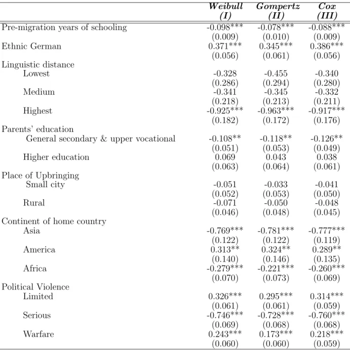
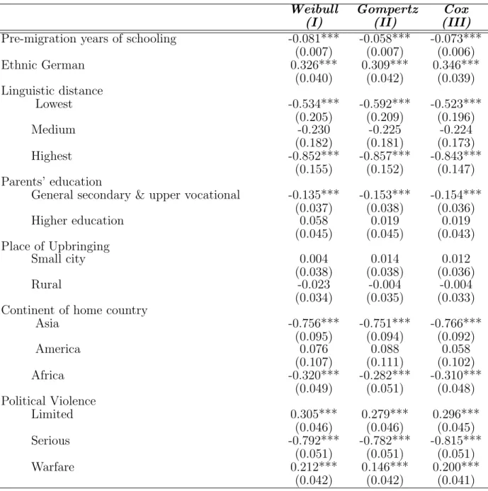
Timing of Migration The timing of migration estimates for men only and for the full sample are presented in Tables 1.3 and 1.4, respectively. I estimate three specifications of the timing of migration equation: a Weibull proportional hazard model, a Gompertz proportional hazard model and a Cox proportional hazard model. The differences between the specifications are different distributional assumptions about the baseline hazard. The first specification assumes a Weibull distribution (i.e., λ0(t) =ptp−1), the second assumes a Gompertz distribution (i.e.,λ0(t) = expγt), and in the third,λ0(t) is left unspecified. Based on the estimates in Tables 1.3 and 1.4, the different distributional assumptions do not seem to affect the estimates.
Estimates are also consistent with the theoretical predictions of the model given in Section 1.2. The model predicts that individuals with a higher skill transferability would migrate
at an earlier age. We observe that ethnic Germans, who are likely to be familiar with the culture and language in Germany and have a higher degree of skill transferability have a higher hazard of early migration. On the other hand, individuals with a high linguistic distance and, hence, a low degree of skill transferability migrate late. Estimates also show that immigrants from geographically-distant countries such as in Asia and Africa have a lower hazard of early migration compared to immigrants from Europe. Apart from the cost of migration, immigrants from Asia and Africa are also less likely to be familiar with German culture and customs. Hence, immigrants from these continents have a lower degree of skill transferability and, consequently, migrate later.
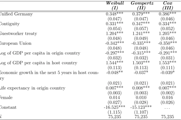
statis-tically significant effect. The estimates of country-level factors of migration are statisstatis-tically significant and in line with our expectations: immigrants from countries that share a border with Germany (contiguity) or those with a Guestworker treaty have a higher hazard of early migration whereas immigrants from origin countries with a higher annual GDP per capita have a lower hazard of early migration.
Interestingly, at any given point of time, the GDP per capita in Germany increases the hazard of early migration but the future economic growth in Germany decreases the hazard. This finding indicates that prospective immigrants postpone migration if they expect a higher economic growth in Germany in the next five years. The estimated effect of political violence at origin is a bit surprising. The hazard of early migration does not monotonically increase with an increase in the level of political violence. Immigrants migrate early when either there is a low level of political violence or there is a war outbreak. The recent Syrian refugee crisis is a testament to how a war can push people to migrate. However, it is puzzling to find that a medium intensity of political violence at origin decreases the hazard of early migration. A possible explanation is that individuals keep postponing the migration in the hope that the situation at origin will improve in the near future.
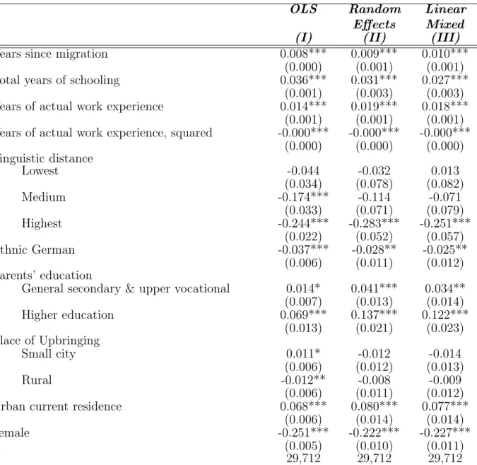
Wage Assimilation The estimates of the wage assimilation equation for men and for the full sample are presented in Tables 1.6 and1.7, respectively. I present three specifications of the wage assimilation equation: ordinary least squares, random effects and a linear mixed model. For the full sample, the wage assimilation equation uses inverse propensity weights obtained from estimating a selection into employment equation (except for the random effects specification, which does not allow using weights).
probability and ethnic Germans have a higher probability of employment. The employment probability increases with the number of years of education and work experience, but de-creases with years since migration. Immigrants with a high linguistic distance compared to those with a zero linguistic distance have a lower employment probability. A surprising result is that immigrants whose parents had higher education are less likely to be employed relative to immigrants whose parents had little or no education.
The estimates of the rate of assimilation in Tables 1.6 and 1.7 are quite similar across the three specifications. The linear mixed model, however, has a slightly higher rate of assimilation than the ordinary least squares and random effects specifications. An additional year of stay increases the hourly wage by less than one percent. This estimate might seem low; however, it falls within the wide range of estimates that have been reported for various countries. There is no consensus in the literature on the magnitude of the average rate of assimilation. For instance,Borjas(1989), using a longitudinal data for immigrants in science and highly professional occupations in United States, found no evidence of assimilation. However,Borjas (1994) used US census data and found the rate of assimilation in the range of 0.7 to 2.1 percent. For United Kingdom, Dustmann and Fabbri (2003) find the rate of assimilation between 3.0 to 3.2 percent. For Germany, Isphording and Otten (2014) use SOEP and find the average rates of assimilation between 2.1 to 1.1 percent. Dustmann(1993) also found a 1.4 percent earnings return on years since migration for temporary migrants. Thus, the reduced form estimate of the average rate of assimilation is comparable to the estimates found by other studies on Germany.
1.5.2 Joint Model Estimates
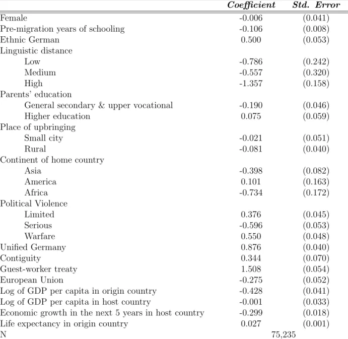
States and Mexico. The immigrants from origin countries that had a Guest worker treaty with Germany have a higher hazard of early migration. On the other hand, immigrants from member countries of European Union migrate late. Also, immigrants are more likely to migrate after the fall of the Berlin wall in a unified Germany.
Similar to the reduced form estimates, we observe that migrants from Asia and Africa are less likely to migrate early relative to European migrants. Also, a low level of political violence and war outbreak increases the hazard of early migration, but a medium level of political violence does not. Among individual characteristics, high linguistic distance, a rural place of ubpringing, and pre-migration years of schooling decrease the hazard of early migration. Being an ethnic German, on the other hand, increases the hazard.
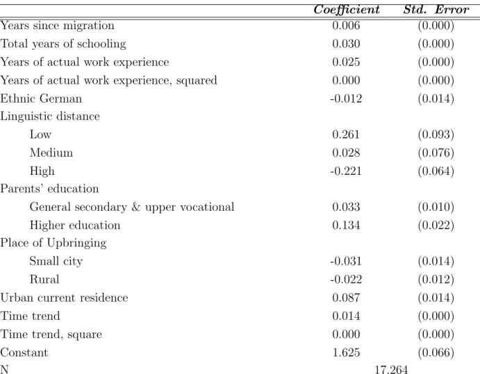
The estimates of wage assimilation using the joint model (see Table 1.9) show that the reduced form estimates of the rate of assimilation are biased upward. We observe that the estimate of the average rate of assimilation from the joint model is nearly half of what is suggested by the linear mixed model and is closer to the ordinary least squares estimate (refer to Table 1.6). The average rate of assimilation in the joint model is 0.6 percent whereas the linear model predicts it to be 1 percent. Thus, the failure to account for selective timing of migration overestimates the actual rate of assimilation. This upward bias is a result of the unaccounted correlation between the propensity of early migration and the individual-specific rates of assimilation. Because the unobserved propensity to migrate early and individual rates of assimilation are positively correlated (refer to Table 1.10), individuals who have a high propensity to migrate early also have high rates of assimilation. Moreover, the individuals with a high propensity to migrate early would appear for a longer duration in the dataset as these individuals migrated at an early age. Thus, the sample disproportionately contains more observations of individuals with a high rate of assimilation. The upward bias is potentially a result of such sample selection.
distance has a negative effect. Among pre-migration individual characteristics, a rural place of upbringing and German ethnicity have a weak negative effect on the wage. However, a better socio-economic status (as indicated by parent’s education) positively affects an immigrant’s wage.
Immigrant quality, Individual Rate of Assimilation and Propensity of Early
Migration The distribution of the individual-specific rate of assimilation in Figure 1.6 shows individual rates of assimilation vary significantly between immigrants. This variation may reflect the differences in the rate or quality of human capital acquisition after migration among immigrants. Even though the average assimilation rate is 0.6 percent , the individual rate of assimilation can be as high as 5 percent and as low as a negative 3.5 percent. Thus, it is clear that the average rate of assimilation masks a remarkable degree of variation in the individual-specific rates of assimilation. A negative rate of assimilation seems puzzling. However, remember that there is a positive rate of return on the years of actual work ex-perience. Thus, immigrant’s wages are not falling with an additional year but the return for an additional year is lower. It is possible that the immigrants with highly transferable pre-migration skills have a negative assimilation as found byChiswick and Miller(2011). On closer inspection, I do observe that negative assimilation mostly occurs for immigrants from Guest-worker countries who could easily use their pre-migration skills in Germany.
consequently, have a higher rate of assimilation. Empirically, Duleep and Regets (2002) have also shown an inverse relationship between the growth of immigrants’ earnings and immigrants’ entry earnings, where entry earnings are used to proxy the immigrant quality.16 Borjas (1999) also predicts a negative correlation when there exists a “relative substi-tutability” between pre- and post-migration human capital. If immigrants can utilize a substantial size of the pre-migration skills in the host country, they would not face a high initial disadvantage in the host country’s labor market. As a result, augmenting human capital stock after migration would be more expensive. Borjas predicts that, in such a case, immigrants would have slower wage growth.
The covariance structure also shows that immigrants who have a higher propensity to migrate early, also have a higher rate of assimilation, thus, indicating a positive correlation. This finding can be explained by two scenarios: (1) individuals with a higher propensity to migrate early invest more in host country specific human capital, or (2) individuals who expect a high wage growth after migration choose to migrate earlier. Although, we cannot separately identify the relative importance of the two cases, it is clear that timing of migration and wage assimilation are not independent.
1.6 Conclusion
This paper provides both theoretical and empirical evidence that the commonly-made exogeneity assumption of years since migration in the host country is incorrect. It is the first paper in the literature to develop and estimate a joint model of timing of migration and economic assimilation. The joint model has two advantages: (1) it accounts for the selective timing of migration; and (2) it estimates the joint distribution of individual-specific rates of assimilation, immigrant quality, and the propensity to migrate early, and reveals the correlation between these components.
individual rates of assimilation are positively correlated. Such findings validate my assertion that the two processes must be estimated together. We also observe that individual rates of assimilation are higher among immigrants who are of comparatively lower quality and have lower skill transferability. Hence, a catch-up effect is observed between low-quality and high-quality migrants. These findings address concerns about immigrant assimilation, especially in recent times when several countries have received an influx of forced migrants. The model predicts that, although forced migrants face an initial disadvantage in the host-country labor-market, they rapidly invest in host-country-specific human capital and eventually reach their potential.
1.7 Tables
Table 1.1: Summary Statistics for Key Variables
Male Female Both
Years since migration 18.274 17.397 17.865
(9.078) (9.011) (9.057)
Total years of schooling 10.261 10.207 10.236
(2.269) (2.532) (2.395)
Years of actual work experience 21.908 12.023 17.302
(11.204) (10.653) (12.010) Linguistic distance
Zero 0.009 0.011 0.010
Low 0.010 0.014 0.012
Medium 0.016 0.013 0.014
High 0.964 0.960 0.962
Ethnic German 0.219 0.263 0.239
Parents’ education
Basic Secondary and Lower Vocational 0.769 0.707 0.740 General secondary & upper vocational 0.162 0.197 0.178
Higher education 0.068 0.940 0.080
Place of Upbringing
City 0.344 0.378 0.360
Small city 0.235 0.243 0.239
Rural 0.420 0.377 0.400
Urban current residence 0.846 0.848 0.847
N 21,668 18,907 40,575
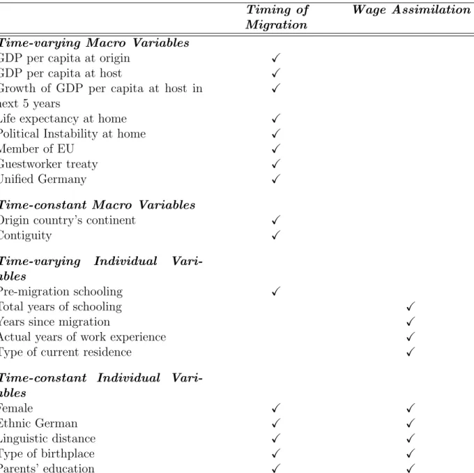
Table 1.2: Key Variables in Timing of Migration and Wage Assimilation Equations Timing of
Migration
Wage Assimilation
Time-varying Macro Variables
GDP per capita at origin X
GDP per capita at host X
Growth of GDP per capita at host in next 5 years
X
Life expectancy at home X
Political Instability at home X
Member of EU X
Guestworker treaty X
Unified Germany X
Time-constant Macro Variables
Origin country’s continent X
Contiguity X
Time-varying Individual Vari-ables
Pre-migration schooling X
Total years of schooling X
Years since migration X
Actual years of work experience X
Type of current residence X
Time-constant Individual Vari-ables
Female X X
Ethnic German X X
Linguistic distance X X
Type of birthplace X X
Parents’ education X X