Sparse Regression Incorporating Graphical Structure among
Predictors
Guan Yu and Yufeng Liu*
Guan Yu is Ph.D. Candidate, Department of Statistics and Operations Research. Yufeng Liu is Professor, Department of Statistics and Operations Research, Carolina Center for Genome Science, Department of Biostatistics, University of North Carolina at Chapel Hill, NC 27599
Abstract
With the abundance of high dimensional data in various disciplines, sparse regularized techniques are very popular these days. In this paper, we make use of the structure information among predictors to improve sparse regression models. Typically, such structure information can be modeled by the connectivity of an undirected graph using all predictors as nodes of the graph. Most existing methods use this undirected graph edge-by-edge to encourage the regression coefficients of corresponding connected predictors to be similar. However, such methods do not directly utilize the neighborhood information of the graph. Furthermore, if there are more edges in the predictor graph, the corresponding regularization term will be more complicate. In this paper, we incorporate the graph information node-by-node, instead of edge-by-edge as used in most existing methods. Our proposed method is very general and it includes adaptive Lasso, group Lasso, and ridge regression as special cases. Both theoretical and numerical studies demonstrate the effectiveness of the proposed method for simultaneous estimation, prediction and model selection.
Keywords
Graph; Lasso; Model selection; Prediction; Sparse regression
1 Introduction
Linear regression plays a fundamental role in statistics. It is widely used in many different scientific areas. Under the standard setting with the sample size n larger than the dimension p, the commonly used ordinary least squares (OLS) estimator for the p dimensional coefficient vector β0 often works well. On the other hand, it is also well known that OLS
often leads to complicate models with low prediction accuracy when the predictors are highly correlated. Furthermore, for the high dimensional data (p ⪢ n), OLS is not applicable due to the rank deficiency of the design matrix. In order to improve OLS, many penalized methods using regularization in model fitting have been proposed in the literature. For example, classical ridge regression (Hoerl and Kennard (1970)) uses the ridge penalty
HHS Public Access
Author manuscript
J Am Stat Assoc
. Author manuscript; available in PMC 2018 February 28.Published in final edited form as:
J Am Stat Assoc. 2016 ; 111(514): 707–720. doi:10.1080/01621459.2015.1034319.
A
uthor Man
uscr
ipt
A
uthor Man
uscr
ipt
A
uthor Man
uscr
ipt
A
uthor Man
uscr
to achieve better prediction performance through a bias-variance trade-off. The
popular Lasso method (Tibshirani (1996)) uses the l1 penalty to perform
continuous shrinkage and automatic variable selection simultaneously. It is known from the literature that Lasso has many good theoretical properties such as model selection
consistency (Zhao and Yu (2006)), estimation consistency (Knight and Fu (2000)), and persistence property for prediction (Greenshtein (2006)). However, Lasso also has some limitations. For example, the shrinkage introduced by Lasso results in significant bias towards 0 for large regression coefficients (Fan and Li (2001)). In the presence of some highly correlated variables, Lasso tends to select only one of those variables (Zou and Hastie (2005)).
Besides the Lasso, a lot of other penalized methods have been proposed for simultaneous variable selection and estimation. For example, Fan and Li (2001) introduced the smoothly clipped absolute deviation (SCAD) method. Zou and Hastie (2005) proposed the Elastic net method and Zou (2006) proposed the adaptive Lasso estimator. Wang et al. (2007) utilized the least absolute deviation Lasso for robust regression. Liu and Wu (2007) used a new penalty that combines the l0 and l1 penalties. Witten and Tibshirani (2009) proposed the
Scout method which includes many penalized methods as special cases. Zhang (2010) studied the minimax concave penalty (MCP) which is a nearly unbiased method for penalized variable selection.
Despite the vast literature on sparse regression, few methods use the structure information of the predictors which can be modeled by the connectivity of an undirected graph. It would be very interesting and useful to study how to use this structure information to improve the performance of variable selection, estimation and prediction. In general, we can get the structure information of the predictors from prior information or estimation. For example, many biological studies have shown that there may exist some regulatory relationships between genes (Li and Li (2008)). An increasing amount of information about gene interaction is organized in databases (Subramanian et al. (2005)). This biological
information can be used to construct the predictor graph where nodes represent genes and edges indicate regulatory relationships. If the prior information is not available in some applications, we can construct the predictor graph by sparse estimation of the covariance (or precision) matrix of the predictors (Yuan and Lin (2007); Friedman et al. (2008); Cai et al. (2011)).
Since the predictor graph can not be represented as some non-overlapping groups, the traditional group Lasso method (Yuan and Lin (2006)) cannot make full use of this complicate structure information. To use the entire predictor graph information, most existing methods use the graph edge-by-edge, through adding some penalty terms to
encourage coefficients and to be similar for predictors i and j connected by an edge.
One type of methods encourages and to be zero or nonzero simultaneously. For
example, OSCAR (Bondell and Reich (2008)) uses the l∞ penalty for every pair of different predictors. Yang et al. (2012) generalized OSCAR to graph OSCAR (GOSCAR) which only uses the l∞ penalty for those pairs of predictors connected by an
A
uthor Man
uscr
ipt
A
uthor Man
uscr
ipt
A
uthor Man
uscr
ipt
A
uthor Man
uscr
edge in the given predictor graph. Pan et al. (2010) introduced a weighted Lγ-regularization. Kim et al. (2013) proposed a new non-convex penalty term based on the truncated lasso
penalty. Another type of methods uses some penalty terms to encourage and have similar values or absolute values. For example, GRACE (Li and Li (2008)) uses the penalty
to smooth the weighted over the predictor graph, where di is the
degree of predictor i. GFlasso (Kim and Xing (2009)) utilizes the penalty
where is the sample correlation coefficient between predictors i and j. Zhang et al. (2013) proposed the logistic graph Laplacian net. Other methods of this type include Yang et al. (2012) and Zhu et al. (2013) which use some non-convex penalty terms
to encourage and to be similar. Although penalized methods using the predictor graph edge-by-edge are promising in improving regression performance, they also have some drawbacks. On the one hand, these methods do not directly utilize the neighborhood information of the graph. For each neighborhood, it can be preferable to use the
corresponding edges jointly rather than separately. On the other hand, the penalty terms in these methods will be more complicate if there are more edges in the graph.
In this paper, instead of using the predictor graph edge-by-edge, we propose a new method, namely Sparse Regression Incorporating Graphical structure among predictors (SRIG), using the graph node-by-node. Specifically, according to the predictor graph G, we assume that there is a latent decomposition of β0 into p parts V(1), V(2), …, V(p) such that
and each V(i) ∈ Rp. The proposed SRIG imposes a penalty to shrink some Vi
to 0 while the other Vi's satisfy , where is a set including predictor i and its
neighbors in graph G. For SRIG, if one predictor is important for prediction, the other predictors connected to it are also encouraged to be in the model. Note that our proposed SRIG method is a graph based penalized regression method with a very different motivation, although the corresponding optimization problem can be formulated as a special case of the Latent Group Lasso approach (Obozinski et al. (2011)) with each neighborhood as a group. For computation, besides introducing the predictor duplication method shown in Obozinski et al. (2011), we also propose a new iterative proximal algorithm which is very efficient for high dimensional data. Our theoretical study shows that SRIG has close connections with several existing methods: (1) It is the same as the adaptive Lasso method when the predictor graph G has no edge; (2) It is equivalent to the group Lasso method when G consists of multiple complete subgraphs; (3) It has the same nonzero solution set as the ridge regression when G is a complete graph. Under some conditions, SRIG enjoys model selection consistency and acquires tight finite sample bounds for both estimation and prediction. In order to evaluate the performance of SRIG, we compare SRIG with many existing methods. Simulation examples with different kinds of predictor graphs are studied. We also analyze a dataset from the Alzheimer's Disease Neuroimaging Initiative (ADNI) database (www.loni.ucla.edu/ADNI). The structural magnetic resonance imaging (MRI) features are used to predict the mini-mental state examination (MMSE) score (Folstein et al. (1975)). Both the simulation results and the real data application indicate that SRIG has competitive performance in estimation, prediction and model selection.
A
uthor Man
uscr
ipt
A
uthor Man
uscr
ipt
A
uthor Man
uscr
ipt
A
uthor Man
uscr
The rest of the paper is organized as follows. In Section 2, we motivate and introduce our proposed SRIG method. In Section 3, we introduce two methods to solve the optimization problem. In Section 4, we show some theoretical properties. In Sections 5 and 6, we demonstrate the use of SRIG on simulated data and the ADNI dataset. We conclude this paper with some discussion in Section 7. Technical proofs are provided in the supplementary materials.
2 Motivation and Methodology
Consider the following linear regression model:
(1)
where ϵ = (ϵ1, ϵ2, …, ϵn)T is a vector of i.i.d. random variables with mean 0 and variance
σ2. Here, is a vector of true coefficients, Y = (y
1, y2, …, yn)T is an n
× 1 response and X = (X1, X2, …, Xp) = (x1, x2, …, xn)T is an n × p design matrix.
For motivation, we first consider the random design setting and assume that each xk follows some multivariate distribution with mean 0p×1 and covariance matrix Σ. The design matrix X
is assumed to be independent of the random error ϵ. Furthermore, denote Ω = (ωij)i,j=1,2,…,p
= Σ−1 and Σ
xy = (c1, c2, …, cp)T ∈ Rp as the cross-covariance vector between xk and yk.
By model (1) and the definition of cross-covariance, we have
Then, we observe that β0 = Σ−1Σ
xy = ΩΣxy, where Ω measures partial correlations among
predictors, and Σxy reflects the marginal correlations between predictors and response
variable. From β0 = ΩΣ
xy, we have
Note that β0 is the sum of p parts, {(c
iω1i, ciω2i, …, ciωpi)T : 1 ≤ i ≤ p}. For the ith part,
(ciω1i, ciω2i, …, ciωpi)T, there is a common factor ci. If the ith predictor and the response variable are uncorrelated marginally, then ci will be 0 and all the components in the ith part of β0 will be 0 simultaneously. Furthermore, if c
i is not zero and the predictor graph is
defined by Ω, then the support of (ciω1i, ciω2i, …, ciωpi)T becomes , which is a set
including predictor i and its neighbors in the predictor graph. Thus, instead of focusing on β0 in the model, we consider a latent decomposition of β0 into p parts. After choosing the
candidate non-zero components in each part based on , we use the group
A
uthor Man
uscr
ipt
A
uthor Man
uscr
ipt
A
uthor Man
uscr
ipt
A
uthor Man
uscr
sparsity constraint to encourage the selected components in each part to be zero or nonzero simultaneously.
The above idea can be generalized for an arbitrary predictor graph constructed by the prior information or estimation from data. Given the predictor graph G, we define a p × p adjacency matrix E, where Eij = 1 if predictors i and j are connected and Eij = 0 otherwise.
For each i, we set Eii = 1 and acquire the neighborhood set . As the previous
case, we assume that β0 can be decomposed into
Here, the ith part is whose candidate nonzero components
are . We can view as the effect arising from the marginal
correlation between the ith predictor and the response variable. If they are uncorrelated,
will be zero for each and the components in the set will be zero simultaneously. Therefore, after choosing the candidate non-zero components in each part based on , it is reasonable to use the group sparsity constraint to encourage the selected components in each part to be zero or nonzero together. Based on this
motivating idea, given the training data (Y, X) and predictor graph G, we propose a new method, Sparse Regression Incorporating Graphical structure among predictors (SRIG), shown as follows.
Here, we use τi to denote the positive weight for the ith group. The choice of τi will be
discussed in Section 4.4.
3 Computation
In this section, we introduce two methods to solve the problem (2). One is the predictor duplication (PD) method proposed in Obozinski et al. (2011) and another one is our proposed iterative proximal (IP) algorithm. The predictor duplication method transforms (2) to a traditional group Lasso problem by duplicating predictors while our proposed new algorithm solves problem (2) directly without duplicating predictors.
3.1 Predictor duplication method
Denote as the sub-vector of V(i) with indices in and as the
sub-matrix of X with column indices in . Denote and
. Then, we can check that , and problem (2) is equivalent to the following group Lasso problem:
A
uthor Man
uscr
ipt
A
uthor Man
uscr
ipt
A
uthor Man
uscr
ipt
A
uthor Man
uscr
(3)
Many efficient R packages such as grpreg (Breheny and Huang (2009)) and gglasso (Yang
and Zou (2013)) can be used to solve problem (3). After setting for each i, we have
. Note that in some cases, some neighborhoods maybe exactly the
same. Then, the vectors are indistinguishable and therefore the decomposition of β (i.e., {V(1), V(2), …, V(p)}) is not unique. In this case, although we can not estimate
each vector in stably, we can estimate directly and stably using the
penalty term . Since , different decompositions of β
lead to the same estimation of β.
The predictor duplication method shown above is very convenient to use and has good performance in general. However, when the dimension is high and at the same time the predictor graph is not very sparse, there will be a lot of duplicated predictors in (3) and therefore the predictor duplication method can be inefficient (Obozinski et al. (2011)). In the following Section 3.2, we will propose a new iterative proximal algorithm which does not duplicate predictors. It is stable and very efficient for the high dimensional data, especially when the predictor graph can be decomposed into several disconnected components.
3.2 Iterative proximal algorithm
Given the predictor graph G and positive weights τi's, for β ∈ Rp, define
(4)
We can show that ∥β∥G,τ is a norm (Obozinski et al. (2011)) and (2) is equivalent to
(5)
In problem (5), the squared loss function is strictly convex and differentiable. In addition, ∥β∥G,τ is a norm and therefore convex. Thus, we can use the Fast Iterative Shrinkage
Thresholding Algorithm (FISTA) (Beck and Teboulle (2009)) to solve it. For our specific problem (5), we propose the following iterative proximal algorithm.
By Theorem 4.4 in Beck and Teboulle (2009), the sequences {β(m)} generated via (6) will
converge to the optimal solution with rate O(1/m2). The most time consuming step in the
A
uthor Man
uscr
ipt
A
uthor Man
uscr
ipt
A
uthor Man
uscr
ipt
A
uthor Man
uscr
above IP algorithm is to compute the projection of h(m) onto the convex set . Follow the proofs of Lemmas 1 and 2 in Villa et al. (2014), we can show that
(7)
Thus, (6) is used to compute the proximal operator of defined as
(8)
In (6), based on the number of elements in , denoted as , we use different methods
flexibly to find the projection of h(m) onto the convex set efficiently. If is small (e.g., smaller than p/10 in our simulation study), we calculate the projection by solving the
dual problem via the Bertsekas's projected Newton method (Villa et al. (2014)). If is large (e.g., larger than p/10), we propose to find the projection by the Parallel Dykstra-like proximal algorithm as shown in Combettes and Pesquet (2011). The details about these two algorithms are shown in the supplementary materials. Furthermore, we note that this IP algorithm is scalable to large scale problems when the predictor graph G can be decomposed into several components (i.e., the covariance/precision matrix is block diagonal). Denote the disconnected components in G as G1, G2, …, GK with node sets C1, C2, …, CK respectively.
In this case, we can compute the proximal operator (8) efficiently by solving the following K subproblems in parallel:
where βck, τck, are sub-vectors of β, τ, and h(m), respectively.
The above parallel computation can potentially save a lot of computational cost. In Section 5.3, we will compare the computational costs of the PD method with our IP algorithm using several simulated examples. In general, the predictor duplication method is very efficient for small data sets. However, when the dimension is high and the predictor graph G is not very sparse, our proposed IP algorithm is much faster than the predictor duplication method. Furthermore, in some cases, the predictor duplication method may break down since it requires immense working memory.
A
uthor Man
uscr
ipt
A
uthor Man
uscr
ipt
A
uthor Man
uscr
ipt
A
uthor Man
uscr
4 Theoretical Properties
In this section, we study the theoretical properties of our proposed SRIG method. For theoretical study, it is convenient to consider (5) as the objective function. In (5), the optimal decomposition of β minimizing ∥β∥G,τ always exists, but may not be unique (Obozinski et
al. (2011)). Denote , , and s0 = |J0| as the true nonzero
coefficient set, the true zero coefficient set, and the number of true nonzero coefficients, respectively. For each β ∈ Rp, denote as the set of all optimal decompositions of β,
and KG,τ(β) as the number of nonzero V(i)'s in the optimal decomposition of β which has the
minimal number of nonzero V(i)'s, i.e.,
. Denote KG,τ = supsupp(β)⊆J0
KG,τ(β). We can check that KG,τ = s0 if the graph G has no edge, KG,τ = K0 if G consists of
some disconnected complete subgraphs and J0 is the union of K0 node sets of those disconnected subgraphs.
4.1 Subgradient conditions
The following proposition shows the subgradient conditions for problem (5).
Proposition 1 A vector β ∈ Rp is a solution of (5) if and only if β can be decomposed as
where V(i)'s satisfy that, for all 1 ≤ i ≤ p, (a) ; (b) either and
, or and .
The subgradient conditions shown above are similar to the subgradient conditions for the latent group Lasso (Obozinski et al. (2011)) and group Lasso (Nardi and Rinaldo (2008)).
According to Proposition 1, if is a solution of problem (2), then for
each i, either or . Thus, the estimate acquired by
our proposed SRIG method has the same decomposition pattern as we discussed in Section 2.
4.2 Connections with some existing methods
The following proposition shows the connections between our proposed SRIG method and several other existing penalized methods when the given predictor graph has some special structures.
Proposition 2 (a) If the predictor graph has no edge, the proposed SRIG method is the same as the adaptive Lasso method for each tuning parameter λ; (b) If the predictor graph consists of K disconnected complete subgraphs, our proposed SRIG method is equivalent to the group Lasso method for each λ; (c) If the predictor graph is a complete graph, our proposed SRIG method has the same nonzero solution set as the ridge regression, i.e., for each
A
uthor Man
uscr
ipt
A
uthor Man
uscr
ipt
A
uthor Man
uscr
ipt
A
uthor Man
uscr
nonzero solution acquired by ridge regression (or SRIG), SRIG (or ridge regression) could acquire the same solution using a different tuning parameter.
Proposition 2 indicates that the proposed SRIG method includes adaptive Lasso, group Lasso, and ridge regression as special cases. It is much more general and can handle any arbitrary predictor graph structure.
4.3 Finite Sample Bounds
In this section, we derive the oracle inequalities for the prediction and estimation loss of our proposed SRIG method. The design matrix X is treated as fixed in this subsection. For a given graph G, positive weights τj's and subset J ⊂ {1, 2 …, p}, denote as the set
of all optimal decompositions of β such that . For each
1 ≤ i ≤ p, denote di as the number of predictors in the neighborhood , i.e., . The following conditions are considered in this section.
(A1)
The errors .
(A2) The neighborhood for each i ∈ J0. (A3) There exists κ > 0 such that
Note that condition (A1) is a common condition for linear regression. Condition (A2) assumes that the given predictor graph G is “consistent” with β0, i.e., predictors connected to
the useful predictor are also useful. Condition (A3) is similar to the restricted eigenvalue conditions used for the group Lasso (Nardi and Rinaldo (2008); Lounici et al. (2011)) and the overlapped group Lasso (Percival (2012)). It is used to analyze the l2 consistency property of both estimation and prediction.
Theorem 1 Suppose that conditions (A1), (A2) and (A3) are satisfied. Let τ* = min1≤i≤p τi
and denote ηi as the positive square root of the largest eigenvalue of . If we
choose where A > 8, then, for any optimal solution of problem (5), we have
with probability at least 1 − p1−q, where .
A
uthor Man
uscr
ipt
A
uthor Man
uscr
ipt
A
uthor Man
uscr
ipt
A
uthor Man
uscr
Remark 1. Note that the above results are very general and have close connections with the results shown in the literature. For example, when the predictor graph G has no edge, we
have KG,τ = s0 and if τi = 1 for each i. Theorem 1 indicates that our
proposed SRIG method acquires the same rates of prediction and estimation as the results shown in Bickel et al. (2009) for the Lasso method. When the given graph G consists of some disconnected complete subgraphs and J0 is the union of K0 node sets of those disconnected subgraphs, we have KG,τ = K0. In this case, we can also recover the results
shown in Nardi and Rinaldo (2008) and Lounici et al. (2011) for the group Lasso.
4.4 Model Selection Consistency
In this section, we first study the model selection consistency for the case with a fixed dimension p. Then, we study the high dimensional case which allows p to grow with n. Both fixed design and random design are considered in these two cases. For every β ∈ Rp, denote
βJ0 and as the sub-vectors of β with indices in J0 and respectively.
For the fixed p case, we use the following two common conditions:
(A4) As n → ∞, , where is a positive matrix.
(A5) The errors ϵ1, ϵ2, …, ϵn are i.i.d. random variables with mean 0 and finite
variance σ2.
Theorem 2 Assume conditions (A2), (A4) and (A5) hold. Suppose the tuning parameter λ and weights τi's are chosen such that and n(γ+1)/2λ → ∞ for some γ > 0.
Furthermore, τj = O(1) for each j ∈ J0 and lim infn→∞ n−γ/2τj > 0 for each . Then,
with dimension p fixed, as n → ∞, we have
where is the sub-matrix of consisting of the entries with row and column indices in J0.
Remark 2. Theorem 2 indicates that our proposed SRIG method is model selection consistent for the fixed p case. It also provides a guideline on how to choose the positive weight τj. When n > p, similar to the weights used for the Adaptive Lasso (Zou (2006)), we
can choose , where is any -consistent estimate of . Note that Theorem 2 can be extended to the random design setting naturally.
Corollary 1 Consider the random design setting where x1, x2, …, xn are i.i.d. samples from a
multivariate distribution with mean 0 and covariance matrix Σ. Assume that the design matrix X and the errors ϵ are independent. Suppose conditions (A2) and (A5) hold. The tuning parameter λ and weights τi's are chosen such that and n(γ+1)/2λ → ∞ for
some γ > 0. Furthermore, τj = O(1) for each j ∈ J0 and lim infn→∞ n−γ/2τj > 0 for each
. Then, with p fixed, as n → ∞, we have
A
uthor Man
uscr
ipt
A
uthor Man
uscr
ipt
A
uthor Man
uscr
ipt
A
uthor Man
uscr
where ΣJ0,J0 is the sub-matrix of Σ consisting of the entries with row and column indices in J0.
For the high dimensional case which allows the dimension p to grow with n, if the design matrix X is considered to be fixed, we need the following conditions:
(A6) The number of nonzero coefficients s0 = O(nδ0) for some constant δ0 ∈ (0, 1). (A7)
There exists a constant Q1 > 0 such that for each n. (A8)
There exists a constant Q2 > 0 such that the smallest eigenvalue of is larger than Q2 for each n.
(A9)
There exists a constant ξ ∈ (0, 1) such that ,
where for a k × m matrix M, ∥M∥∞ is defined as .
Note that condition (A6) is a common sparsity assumption for the high dimensional regression problem. Condition (A7) can be satisfied by normalizing each predictor.
Condition (A8) guarantees that the matrix is invertible and its inverse behaves well. The main condition (A9) is similar to the strong irrepresentable condition used for Lasso (Zhao and Yu (2006)).
Theorem 3 Assume conditions (A1), (A2), (A6)-(A9) hold. Suppose the weight τj is chosen
to be for each j, where the mj's satisfy that maxj∈J0 mj = Op(1) and
for some γ > δ0. Furthermore, the selected tuning
parameter λ and the minimum absolute nonzero coefficient satisfy that, as n → ∞ and p = p(n) → ∞,
Then, as n → ∞ and p = p(n) → ∞, there exists a solution to (5) such that
with probability tending to 1, where sign(·) maps a positive entry to 1, a negative entry to −1 and zero to zero.
Remark 3. For clarification, we note that many quantities such as p, s0, λ, τj and dj depend on n. We use simple notation here for convenience. Theorem 3 indicates that our proposed SRIG method is model selection consistent for the high dimensional case. For example,
A
uthor Man
uscr
ipt
A
uthor Man
uscr
ipt
A
uthor Man
uscr
ipt
A
uthor Man
uscr
suppose the dimension p = O(enδ1) for some constant δ1 ∈ (0, 1). Furthermore, for
sufficiently large n, the minimum absolute nonzero coefficient satisfies that
for some constants C1 > 0 and δ2 > δ1. If we select the weights τj's as
shown in the theorem and the tuning parameter λ = C2n(δ1−2δ0−1)/2 for some constant C2 >
0, then by Theorem 3 we can show that there exists a solution such that
with probability tending to 1. In the high dimensional case with p ⪢ n,
our simulation study suggests that choosing works well. The positive parameter γ can be chosen by cross validation.
In Theorem 3, as the Lasso method, we use the irrepresentable condition (A9). In fact, we can also use the following condition (A9′) in order to reflect the use of the weights τj's.
Following the same proof of Theorem 3, we can achieve the model selection consistency as shown in Corollary 2.
(A9′) There exists a constant ξ ∈ (0, 1) such that for each , we have
Corollary 2 Assume conditions (A1), (A2), (A6)–(A8), (A9′) hold. Suppose the weight τj's
satisfy that . Furthermore, the selected tuning parameter λ and the
minimum absolute nonzero coefficient satisfy the same conditions in Theorem 3, then, as n → ∞ and p = p(n) → ∞, there exists a solution to (5) such that
with probability tending to 1.
Theorem 3 considers the fixed design setting. It can be extended to the random design setting as well. For that setting, the conditions (A6)-(A9) are replaced by the following conditions.
(A10)
Let with Σjj = 1 for each j. Furthermore, assume
that X and ϵ are independent. The dimension , where .
(A11) Restricted eigenvalue assumption:
(A12)
The number of true nonzero coefficients .
Note that conditions (A10)-(A12) are common conditions used in the literature for the random design setting (Bickel et al. (2009); Zhou et al. (2009)). Under these conditions, we can show that our proposed SRIG method is also model selection consistent for the high dimensional case with random design.
A
uthor Man
uscr
ipt
A
uthor Man
uscr
ipt
A
uthor Man
uscr
ipt
A
uthor Man
uscr
Theorem 4 Assume conditions (A1), (A2), (A10)-(A12) hold. Suppose the weight τj is
chosen to be for each j, where .
Furthermore, the selected tuning parameter λ and the minimum absolute nonzero coefficient satisfy that, as n → ∞ and p = p(n) → ∞,
Then, as n → ∞ and p = p(n) → ∞, there exists a solution to (5) such that
with probability tending to 1, where sign(·) maps a positive entry to 1, a negative entry to −1 and zero to zero.
Remark 4. Under conditions (A10)-(A12), we can show that condition (A7) is satisfied with
, condition (A8) is satisfied with Q2 = Λmin(s0), and
, with probability greater than 1 − 1/p2.
Based on these results, we can use a similar proof of Theorem 3 to prove Theorem 4.
5 Simulation Study
In this section, we first compare our proposed SRIG method with many existing methods. Then, we conduct a sensitivity study of the SRIG method. Finally, we compare the
computational costs of the predictor duplication method and our proposed iterative proximal algorithm using some simulated examples.
5.1 Performance Comparison
To examine the performance of SRIG, we compare it with many other methods on three examples. Firstly, we compare SRIG with popular penalized methods such as Lasso, Ridge regression, Adaptive Lasso (ALasso) and Elastic net (Enet) which do not use the predictor graph structure information directly. Secondly, we compare SRIG with some existing methods using the predictor structure information. The competitors are GRACE (Li and Li (2008)) and GOSCAR (Yang et al. (2012)). Thirdly, we compare SRIG with other latent component approaches such as principal component regression (PCR) and sparse partial least squares (SPLS) using the R packages pls (Mevik and Wehrens (2007)) and spls (Chung et al. (2012)), respectively. In this simulation study, the predictor graph is defined by the precision matrix of the predictors. The performance of GRACE, GOSCAR and SRIG using both the estimated predictor graph and the oracle true predictor graph are evaluated on all examples. We denote GRACE-O, GOSCAR-O and SRIG-O as the GRACE, GOSCAR and SRIG methods using the true predictor graph, respectively. For comparison, we also show the performance of the least square method based on the true model, which is denoted as LS-O.
A
uthor Man
uscr
ipt
A
uthor Man
uscr
ipt
A
uthor Man
uscr
ipt
A
uthor Man
uscr
We generate data from model (1) with the errors . For each example, our simulated data include a training set, an independent validation set and an independent test set. All the models are fitted on the training data only. The validation data are used to choose the tuning parameter and the test data set is used to evaluate different methods. We use the notation ./././ to show the sample sizes in the training, validation and test sets, respectively. For each example, we consider three cases: (I) 40/40/400, (II) 80/80/400 and (III) 120/120/400. For each case, we repeat the simulation 50 times. The predictor graph is estimated by the graphical Lasso method (Friedman et al. (2008)) only using the training data in all cases.
Example 1 (Ω is block diagonal) p = 100, s0 = 15, σ = 5, and the true coefficient vector β0 = (3, 3, ⋯, 3, 0, 0, ⋯, 0)T. The predictors are generated as:
where , j = 1, 2, …, 15.
Example 2 ( Ω is banded) p = 100, σ = 10, and β0 is the same as the β0 used in Example 1. The predictors (X1, X2, …, Xp)T ~ N(0, Σ) with Σij = 0.5|i−j|.
For this example, we have ωii = 1.333, ωij = −0.667 if |i − j| = 1 and ωij = 0
if |i − j| > 1.
Example 3 ( Ω is sparse) p = 100, σ = 5, and the predictors (X1, X2, …, Xp)T ~ N(0, Ω −1), where = Ω = B + δI. Each off-diagonal entry in B is generated
independently and equals to 0.5 with probability 0.05, or 0 with probability 0.95. The diagonal entry of B is 0. Here, δ is chosen such that the
conditional number of Ω is equal to p. Finally, Ω is standardized to have unit diagonals. We set β0 = ΩΣ
xy, where Σxy = (c1, c2, …, cp)T with ci = 10
for the predictors having the top four largest degrees and ci = 0 otherwise.
To evaluate different methods, we use the following measures:
• l
2 distance ; •
Relative prediction error (RPE) , where
Xtest is the test samples and Ntest is the number of test samples; • False positive rate (FPR) and False negative rate (FNR);
A
uthor Man
uscr
ipt
A
uthor Man
uscr
ipt
A
uthor Man
uscr
ipt
A
uthor Man
uscr
•
Nonzero match ratio , which
is used to check whether the estimated coefficients of two connected useful predictors are both nonzero; Zero match ratio
, which is used to check whether the estimated coefficients of two connected useless predictors are both zero. We use NMR and ZMR when there is at least one edge connecting two useful predictors and one edge connecting two useless predictors. Thus, these two ratios are well defined and always between 0 and 1.
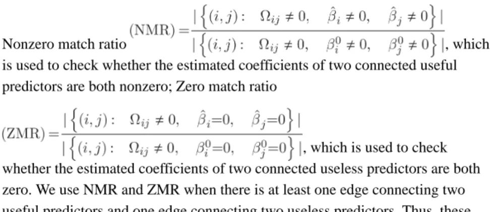
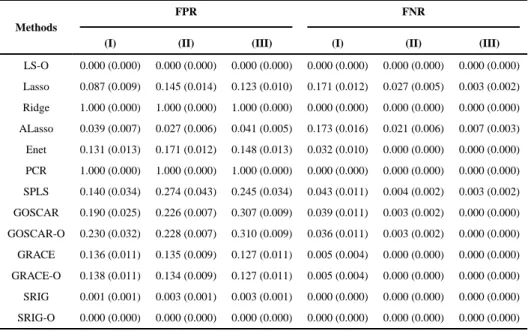
Figure 1 shows the true predictor graphs (defined by Ω) of these three examples. The numbers of edges for these three graphs are 30, 99 and 243 respectively. Such graphs were also studied in the literature previously (Yang et al. (2012); Cai et al. (2011)). It is very interesting to study whether the structure information represented by these predictor graphs could be used to improve the performance of estimation, prediction and model selection. Tables 1–2 show the performance comparison for Example 1. The comparison results indicate that the Elastic net method acquires better estimation and prediction than Lasso, ridge regression and adaptive Lasso methods by using a linear combination of l1 and ridge penalty. The GOSCAR and GRACE methods further improve the performance of estimation and prediction benefiting from using the addtional estimated predictor graph directly. However, Elastic net, GOSCAR and GRACE methods still have relatively high FPR. Compared with the other methods (not including methods using the true predictor graph), our proposed SRIG method delivers the best performance of estimation and prediction. Furthermore, SRIG almost always identifies the true model perfectly for this example. Since the estimated predictor graph for this example is almost the same as the true predictor graph, the performance of GOSCAR-O, GRACE-O and SRIG-O are similar to those of GOSCAR, GRACE and SRIG, respectively. Due to the strong correlation between different important predictors, the performance of LS-O method on this example is not very good. Compared with LS-O, our SRIG method still acquires competitive performance.
Tables 3–4 display the results for Example 2. As Example 1, the Elastic net method has better performance of estimation and prediction than Lasso and ridge regression. For the cases with relative large sample sizes, the adaptive Lasso method acquires better prediction than the Elastic net method. GOSCAR, GRACE and our proposed SRIG obtain better estimation and prediction than the methods not incorporating the additional predictor graph information. Methods using the true predictor graph acquire better estimation and prediction than those methods using estimated predictor graph, especially for the small sample cases (I and II). Compared with GOSCAR (GOSCAR-O) and GRACE (GRACE-O), our proposed SRIG (SRIG-O) has competitive performance of estimation and prediction. Furthermore, the results in Table 4 show that our proposed SRIG-O method acquires much lower FPR than the GOSCAR-O and GRACE-O methods. This indicates that GRACE and GOSCAR methods using the predictor graph edge-by-edge may lead to poor model selection results, although they can acquire competitive performance for estimation and prediction. Compared
A
uthor Man
uscr
ipt
A
uthor Man
uscr
ipt
A
uthor Man
uscr
ipt
A
uthor Man
uscr
with latent component approaches, SRIG has better performance than PCR while worse performance than SPLS. However, SRIG-O has better performance than PCR and SPLS in most cases.
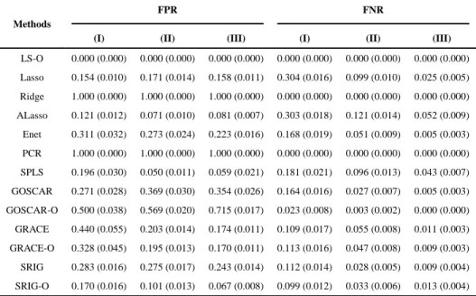
The performance comparison for Example 3 is shown in Tables 5–6. Methods not using the predictor graph have poor performance for both estimation, prediction and model selection, especially for the cases (I) and (II) with smaller n than p. For this example, the performance of estimation and prediction of the Elastic net method is similar to Lasso, ridge regression and adaptive Lasso. When the additional predictor graph information is used, the GRACE method, which can be considered as a graph version of the Elastic net, still does not acquire improved performance. However, GOSCAR benefits from the additional predictor graph information and acquires better performance. Compared with the other methods (not including SRIG-O), our proposed SRIG method has the best results for both estimation, prediction and model selection. As the previous two examples, each method using the true predictor graph performs better than the corresponding method using the estimated graph. For this example, LS-O acquires the best performance and our proposed SRIG-O method has similar results to the LS-O method when the sample size is large.
The comparison results of NMR and ZMR for the cases with sample sizes 40/40/400 are shown in Table 7. The results for the cases with samples sizes 80/80/400 and 120/120/400 are shown in the supplementary materials. Compared with the other methods (except LS-O which uses the underlying true model), our proposed SRIG-O acquires the best performance in most cases. The NMR's of SRIG-O indicate that our proposed SRIG method incorporates most edges between useful predictors efficiently and therefore chooses those connected useful predictors simultaneously. The ZMR's of SRIG-O indicate that our proposed SRIG-O method also makes use of most edges between useless predictors and therefore excludes those connected useless predictors jointly. Overall, for our proposed SRIG method, the estimated pattern (zero or nonzero) among coefficients agrees with the graphical structure very well.
In conclusion, the simulation results indicate that our proposed SRIG method can make use of the structure information among predictors efficiently and performs well for both estimation, prediction and model selection.
5.2 Sensitivity Study
An important condition for our proposed SRIG method is the condition (A2) which requires that the predictor graph G is “consistent” with the true coefficients vector β0, i.e., predictors
connected to the useful predictor are also useful. Since it is difficult to check this condition in practice, it is very important to study the performance of SRIG when the condition (A2) is violated.
To this end, we evaluate the performance of SRIG on a series of data sets with changing predictor graphs. Fix p = 100, σ = 3, s0 = 20, and β0 = (20, 2, 2, ⋯, 2, 0, 0, ⋯, 0)T. For each
p* = 0, 1, …, 30, we generate the predictor matrix X from N(0, Ω−1), where Ω = B + 2|
λmax(B)|Ip. Here, Bii = 2 for each 1 ≤ i ≤ p, B1i = Bi1 = 0.3 for each 1 ≤ i ≤ (s0 + p*), B(s0+1)i
A
uthor Man
uscr
ipt
A
uthor Man
uscr
ipt
A
uthor Man
uscr
ipt
A
uthor Man
uscr
= Bi(s0+1) = 0.3 for each (s0 + 1) ≤ i ≤ p, and Bij = 0 otherwise. λmax(B) is the largest
eigenvalue of the matrix B. Finally, Ω is standardized to have unit diagonals.
For this study, the true precision matrix Ω is used to construct the predictor graph G. The neighborhoods of the useful predictor X1 and the useless predictor Xs0+1 are
and , respectively. The number of
predictors shared by these two neighborhood is
. The condition (A2) is satisfied when p* = 0 and will be violated more and more seriously as p* increases. Based on this example, we study the robustness of SRIG as p* changes gradually from 0 to 30. For each p*, we also evaluate the performance of Lasso method. The sample sizes are fixed as 80/80/400.
Figure 2 shows the performances of SRIG and Lasso method as the number of shared predictors p* increases. It indicates that Lasso method is more robust than our proposed SRIG method to the intersection between the neighborhood of useful predictors and the neighborhood of useless predictors. One possible reason is that Lasso does not use the predictor graph information directly. For our proposed SRIG method, as p* increases, the condition (A2) is more and more violated and the performance of SRIG gets worse. As shown in Figure 2, if the condition (A2) is not violated seriously, our proposed SRIG method still has better performance than the Lasso method. However, if (A2) is violated seriously (i.e., p* > 25), Lasso method performs better than our proposed SRIG method. Besides this study, we also compare SRIG with the other methods on an additional example where the positions of useful predictors in Example 2 are adjusted so that the condition (A2) is much violated. The simulation results (shown in the supplementary materials) indicate that our proposed SRIG method still performs as well as the other methods.
5.3 PD method v.s. IP algorithm
In this subsection, we compare the computational costs of the PD method and our proposed IP algorithm by some examples. Besides the Examples 1-3 shown in Section 5.1, we also consider the following three high dimensional examples:
Example 4 n = 400, p = 1500, s0 = 25, σ = 5, and the true coefficient vector β0 = (1, 1,
⋯, 1, 0, ⋯, 0)T. The predictors are generated as follows.
where , j = 1, 2, …, 50 and Ω* = B + δI. Each off-diagonal
entry in B is generated independently and equals to 0.5 with probability
A
uthor Man
uscr
ipt
A
uthor Man
uscr
ipt
A
uthor Man
uscr
ipt
A
uthor Man
uscr
0.25, or 0 with probability 0.75. The diagonal entry of B is 0. Here, δ is chosen such that the conditional number of Ω* is equal to p − 50. Finally,
Ω* is standardized to have unit diagonals.
Example 5 n = 500, p = 2000 and the other setup is the same as Example 4.
Example 6 n = 600, p = 2500 and the other setup is the same as Example 4.
For these six examples, we use both the PD method (using gglasso R package) and our proposed IP algorithm to compute the solution path of the SRIG method using the true predictor graph. To be specific, we set all the weights τi's to be 1 and compute the set of
solutions corresponding to 100 different values of the tuning parameter λ1 > λ2 > ⋯ > λ100,
where λ1 = ∥XTY/n∥2 which shrinks all the parameters to be 0 and λ100 = 0.05λ1. The
computational times (in seconds) of PD method and IP algorithm are shown in Table 8.
As shown in Table 8, both methods require more time to compute the solution path as the dimension p and the number of edges in the predictor graph increase. When p is small and at the same time the predictor graph G is sparse (e.g., Examples 1-3), the PD method is faster than the IP algorithm. However, for high dimensional data sets with complicate predictor graphs (e.g., Examples 4–6), our proposed IP algorithm is more efficient than the PD method. For Example 6, the PD method using gglasso package breaks down due to out of memory while our proposed IP algorithm still works well. In this case, the proposed IP algorithm is very desirable.
6 Real Data Example
Alzheimer's disease (AD) is one of the most common forms of dementia characterized by progressive cognitive and memory deficits. The increasing incidence of AD makes the disease a very important health issue and a huge financial burden for both patients and governments (Hebert et al. (2001)). In the practical diagnosis of AD, the Mini Mental State Examination (MMSE) (Folstein et al. (1975)) score is a very important reference. MMSE is a brief 30-point questionnaire test that is used to screen for cognitive impairment. It can be used to examine patient's arithmetic, memory and orientation. Generally, any score greater than or equal to 27 points (out of 30) indicates a normal cognition. Below this, MMSE score can indicate severe (≤9 points), moderate (10–18 points) or mild (19–24 points) cognitive impairment (Mungas (1991)). As more and more treatments are being developed and evaluated, it is very important to develop diagnostic and prognostic biomarkers that can predict which individuals are relatively more likely to progress clinically. At present, structural magnetic resonance imaging (MRI) is one of the most popular and powerful techniques for the diagnosis of AD. It is very interesting to use MRI data to predict MMSE score which can be used to diagnose the current disease status of AD.
The dataset we used in this paper is the MRI data and MMSE scores of 51 AD patients and 52 normal controls from the Alzheimer's Disease Neuroimaging Initiative (ADNI) database (www.loni.ucla.edu/ADNI). The image pre-processing steps for the MRI data include anterior commissure posterior commissure correction, intensity inhomogeneity correction, skull stripping, cerebellum removal, spatial segmentation, and registration. After
registration, we obtained the subject-labeled image based a template with 93 manually
A
uthor Man
uscr
ipt
A
uthor Man
uscr
ipt
A
uthor Man
uscr
ipt
A
uthor Man
uscr
labeled regions of interest (ROI) (Kabani et al. (1998)). For each of the 93 ROI in the labeled MRI, we computed the volume of GM tissue as a feature. Therefore, the final dataset has 103 subjects. For each subject, there are one MMSE score and 93 MRI features. We treat MMSE score as the response variable and MRI features as predictors in our model.
To evaluate the performance of our proposed SRIG method, we compare it with Lasso, ridge regression, Adaptive Lasso, Elastic net, GOSCAR, GRACE, PCR and SPLS. The dataset is first scaled to have mean 0 and variance 1 for the MMSE score and each MRI feature. The 10-fold cross validation (CV) is used to evaluate different methods. The predictor (MRI feature) graph G is estimated by the graphical Lasso (Friedman et al. (2008)) only using the training data. Figure 3 shows the estimated MRI feature graph using all the data. There are 93 nodes and 419 edges in this graph. Note that all the models are fitted using training data and evaluated by the mean squared error (MSE) calculated from the testing data. To choose the tuning parameters of different methods, an inner 5-fold CV is used. Considering possible bias due to the random splitting, we repeat 10-CV process ten times. Figure 4 shows the box plot of the averaged mean squared errors of different methods. Compared with the other methods, our proposed SRIG method delivers the best prediction of MMSE scores. The averaged MSE acquired by our proposed SRIG method is 0.5822, which is about 4.6% percent lower than the smallest MSE acquired by the competitors.
For the ten times of our 10-CV process, we acquires 100 models for each method. For our proposed SRIG method, the averaged number of selected MRI features (with estimated coefficients bigger than 0.01) is almost 36. There are seven MRI features always selected by our proposed SRIG method. The feature indices are 4, 19, 22, 30, 69, 80 and 83. Figure 5 shows the multi-slice view of the brain regions corresponding to these seven MRI features. The colored areas are the selected regions. Interestingly, the 30th and 69th features
correspond to the hippocampal regions. The 22th and 83th features correspond to the uncus region and the amygdala region, respectively. These regions are known to be related to AD by many previous studies based on group comparison methods (Jack et al. (1999); Misra et al. (2009); Zhang and Shen (2012)). Moreover, we notice that the 4th, 19th and 80th features relate to the insula right, temporal pole right and middle temporal gyrus right regions, respectively. It would be very interesting to check whether these regions are substantially related to AD by some group comparison studies.
7 Conclusion
In this paper, we propose a new penalized regression method using structure information among predictors. Instead of using the predictor graph edge-by-edge as in the existing literature, our proposed SRIG method uses it node-by-node. Theoretical study shows that SRIG includes adaptive Lasso, group Lasso and ridge regression as special cases. It can make use of the general structure information among predictors efficiently. Furthermore, SRIG acquires tight finite sample bounds for both prediction and estimation. It also enjoys the model selection consistency. Both simulation study and real data analysis show that SRIG is a competitive tool for estimation, prediction and model selection.
A
uthor Man
uscr
ipt
A
uthor Man
uscr
ipt
A
uthor Man
uscr
ipt
A
uthor Man
uscr
Supplementary Material
Refer to Web version on PubMed Central for supplementary material.
Acknowledgments
The authors are supported in part by NIH/NCI grant R01 CA-149569 and NSF grant DMS-1407241. Data used in the preparation of this article were obtained from the Alzheimer's Disease Neuroimaging Initiative (ADNI) database (http://www.loni.ucla.edu/ADNI). As such, the investigators within the ADNI contributed to the design and implementation of ADNI and/or provided data but did not participate in analysis or writing of this report. A complete listing of ADNI investigators is available at http://www.loni.ucla.edu/ADNI/Data/
ADNI_Authorship_List.pdf. The authors thank the editors, the associate editor, and referees for their helpful comments and suggestions.
References
Beck A, Teboulle M. A fast iterative shrinkage-thresholding algorithm for linear inverse problems. SIAM Journal on Imaging Sciences. 2009; 2:183–202.
Bickel PJ, Ritov Y, Tsybakov AB. Simultaneous analysis of Lasso and Dantzig selector. The Annals of Statistics. 2009; 37:1705–1732.
Bondell HD, Reich BJ. Simultaneous Regression Shrinkage, Variable Selection, and Supervised Clustering of Predictors with OSCAR. Biometrics. 2008; 64:115–123. [PubMed: 17608783] Breheny P, Huang J. Penalized methods for bi-level variable selection. Statistics and Its Interface.
2009; 2:369–380. [PubMed: 20640242]
Cai T, Liu W, Luo X. A Constrained l1 Minimization Approach to Sparse Precision Matrix Estimation. Journal of the American Statistical Association. 2011; 106:594–607.
Chung D, Chun H, Keles S. Spls: sparse partial least squares (SPLS) regression and classification. R package, version. 2012; 2:1–1.
Combettes, PL., Pesquet, J-C. Fixed-point algorithms for inverse problems in science and engineering. Springer; 2011. Proximal splitting methods in signal processing; p. 185-212.
Fan J, Li R. Variable selection via nonconcave penalized likelihood and its oracle properties. Journal of the American Statistical Association. 2001; 96:1348–1361.
Folstein MF, Folstein SE, McHugh PR. Mini-mental state: a practical method for grading the cognitive state of patients for the clinician. Journal of Psychiatric Research. 1975; 12:189–198. [PubMed: 1202204]
Friedman J, Hastie T, Tibshirani R. Sparse inverse covariance estimation with the graphical lasso. Biostatistics. 2008; 9:432–441. [PubMed: 18079126]
Greenshtein E. Best subset selection, persistence in high-dimensional statistical learning and optimization under l1 constraint. The Annals of Statistics. 2006; 34:2367–2386.
Hebert LE, Beckett LA, Scherr PA, Evans DA. Annual incidence of Alzheimer disease in the United States projected to the years 2000 through 2050. Alzheimer Disease & Associated Disorders. 2001; 15:169–173. [PubMed: 11723367]
Hoerl AE, Kennard RW. Ridge regression: Biased estimation for nonorthogonal problems. Technometrics. 1970; 12:55–67.
Jack C, Petersen RC, Xu YC, OBrien PC, Smith GE, Ivnik RJ, Boeve BF, Waring SC, Tangalos EG, Kokmen E. Prediction of AD with MRI-based hippocampal volume in mild cognitive impairment. Neurology. 1999; 52:1397–1397. [PubMed: 10227624]
Kabani N, MacDonald D, Holmes C, Evans A. A 3D atlas of the human brain. NeuroImage. 1998; 7:S717.
Kim S, Pan W, Shen X. Network-based penalized regression with application to genomic data. Biometrics. 2013; 69:582–593. [PubMed: 23822182]
Kim S, Xing EP. Statistical Estimation of Correlated Genome Associations to a Quantitative Trait Network. PLoS Genetics. 2009; 5:e1000587. [PubMed: 19680538]
Knight K, Fu W. Asymptotics for lasso-type estimators. Annals of Statistics. 2000:1356–1378.
Li C, Li H. Network-constrained regularization and variable selection for analysis of genomic data. Bioinformatics. 2008; 24:1175–1182. [PubMed: 18310618]
Liu Y, Wu Y. Variable selection via a combination of the L0 and L1 penalties. Journal of Computational and Graphical Statistics. 2007; 16:782–798.
Lounici K, Pontil M, Van De Geer S, Tsybakov AB, et al. Oracle inequalities and optimal inference under group sparsity. The Annals of Statistics. 2011; 39:2164–2204.
Mevik B-H, Wehrens R. The pls package: principal component and partial least squares regression in R. Journal of Statistical Software. 2007; 18:1–24.
Misra C, Fan Y, Davatzikos C. Baseline and longitudinal patterns of brain atrophy in MCI patients, and their use in prediction of short-term conversion to AD: results from ADNI. NeuroImage. 2009; 44:1414–1422.
Mungas D. In-office mental status testing: A practical guide. Geriatrics. 1991; 46
Nardi Y, Rinaldo A. On the asymptotic properties of the group lasso estimator for linear models. Electronic Journal of Statistics. 2008; 2:605–633.
Obozinski, G., Jacob, L., Vert, J-P. Group lasso with overlaps: the latent group lasso approach. 2011. arXiv preprint arXiv:1110.0413
Pan W, Xie B, Shen X. Incorporating predictor network in penalized regression with application to microarray data. Biometrics. 2010; 66:474–484. [PubMed: 19645699]
Percival D. Theoretical properties of the overlapping groups lasso. Electronic Journal of Statistics. 2012; 6:269–288.
Subramanian A, Tamayo P, Mootha VK, Mukherjee S, Ebert BL, Gillette MA, Paulovich A, Pomeroy SL, Golub TR, Lander ES, et al. Gene set enrichment analysis: a knowledge-based approach for interpreting genome-wide expression profiles. Proceedings of the National Academy of Sciences of the United States of America. 2005; 102:15545–15550. [PubMed: 16199517]
Tibshirani R. Regression shrinkage and selection via the lasso. Journal of the Royal Statistical Society: Series B. 1996; 58:267–288.
Villa S, Rosasco L, Mosci S, Verri A. Proximal methods for the latent group lasso penalty. Computational Optimization and Applications. 2014; 58:381–407.
Wang H, Li G, Jiang G. Robust regression shrinkage and consistent variable selection through the LAD-Lasso. Journal of Business & Economic Statistics. 2007; 25:347–355.
Witten DM, Tibshirani R. Covariance-regularized regression and classification for high dimensional problems. Journal of the Royal Statistical Society: Series B (Statistical Methodology). 2009; 71:615–636. [PubMed: 20084176]
Yang, S., Yuan, L., Lai, Y-C., Shen, X., Wonka, P., Ye, J. Feature grouping and selection over an undirected graph. Proceedings of the 18th ACM SIGKDD International Conference on Knowledge Discovery and Data Mining; ACM; 2012. p. 922-930.
Yang, Y., Zou, H. gglasso: Group Lasso Penalized Learning Using A Unified BMD Algorithm. r package version 1.1. 2013.
Yuan M, Lin Y. Model Selection and estimation in regression with grouped variables. Journal of the Royal Statistical Society: Series B. 2006; 68:49–67.
Yuan M, Lin Y. Model selection and estimation in the Gaussian graphical model. Biometrika. 2007; 94:19–35.
Zhang C-H. Nearly unbiased variable selection under minimax concave penalty. The Annals of Statistics. 2010; 38:894–942.
Zhang D, Shen D. Multi-modal multi-task learning for joint prediction of multiple regression and classification variables in Alzheimer's disease. NeuroImage. 2012; 59:895–907. [PubMed: 21992749]
Zhang W, Wan Y.-w. Allen GI, Pang K, Anderson ML, Liu Z. Molecular pathway identification using biological network-regularized logistic models. BMC Genomics. 2013; 14:S7.
Zhao P, Yu B. On model selection consistency of Lasso. The Journal of Machine Learning Research. 2006; 7:2541–2563.
Zhou, S., van de Geer, S., Bühlmann, P. Adaptive Lasso for high dimensional regression and Gaussian graphical modeling. 2009. arXiv preprint arXiv:0903.2515
Zhu Y, Shen X, Pan W. Simultaneous grouping pursuit and feature selection over an undirected graph. Journal of the American Statistical Association. 2013; 108:713–725. [PubMed: 24098061] Zou H. The Adaptive Lasso and Its Oracle Properties. Journal of the American Statistical Association.
2006; 101:1418–1429.
Zou H, Hastie T. Regularization and variable selection via the elastic net. Journal of the Royal Statistical Society: Series B. 2005; 67:301–320.
A
uthor Man
uscr
ipt
A
uthor Man
uscr
ipt
A
uthor Man
uscr
ipt
A
uthor Man
uscr
SRIG Method
Step 1 Find the neighborhoods (note that for each i).
Step 2 Solve the following optimization problem:
(2)
subject to and for each i, where
supp(V(i)) is the support of vector V(i) and ∥ · ∥2 is the l2 norm.
A
uthor Man
uscr
ipt
A
uthor Man
uscr
ipt
A
uthor Man
uscr
ipt
A
uthor Man
uscr
Iterative Proximal (IP) Algorithm
Input The initial estimate β(0) and L= the largest eigenvalue of XTX/n. Step 0 Take Z(1) = β(0) ∈ Rp and t1 = 1.
Step m(m ≥ 1) Compute
(6)
A
uthor Man
uscr
ipt
A
uthor Man
uscr
ipt
A
uthor Man
uscr
ipt
A
uthor Man
uscr
Figure 1.
True predictor graphs of three simulation examples.
A
uthor Man
uscr
ipt
A
uthor Man
uscr
ipt
A
uthor Man
uscr
ipt
A
uthor Man
uscr
Figure 2.
Sensitivity study of the SRIG method.
A
uthor Man
uscr
ipt
A
uthor Man
uscr
ipt
A
uthor Man
uscr
ipt
A
uthor Man
uscr
Figure 3.
Estimated graph of 93 MRI features.
A
uthor Man
uscr
ipt
A
uthor Man
uscr
ipt
A
uthor Man
uscr
ipt
A
uthor Man
uscr
Figure 4.
Comparison of MSE for various methods on the ADNI data set.
A
uthor Man
uscr
ipt
A
uthor Man
uscr
ipt
A
uthor Man
uscr
ipt
A
uthor Man
uscr
Figure 5.
The multi-slice view of seven brain regions always selected by SRIG method.
A
uthor Man
uscr
ipt
A
uthor Man
uscr
ipt
A
uthor Man
uscr
ipt
A
uthor Man
uscr
A
uthor Man
uscr
ipt
A
uthor Man
uscr
ipt
A
uthor Man
uscr
ipt
A
uthor Man
uscr
ipt
Table 1
Performance comparison of estimation and prediction for Example 1.
Methods
l2 distance RPE
(I) (II) (III) (I) (II) (III)
LS-O 8.378 (0.323) 5.014 (0.124) 4.132 (0.142) 0.595 (0.047) 0.212 (0.010) 0.149 (0.010)
Lasso 8.527 (0.199) 5.635 (0.119) 4.328 (0.153) 1.291 (0.087) 0.530 (0.036) 0.274 (0.014)
Ridge 8.166 (0.050) 7.585 (0.039) 4.325 (0.062) 12.336 (0.215) 10.936 (0.144) 0.946 (0.027)
ALasso 8.822 (0.275) 5.570 (0.167) 4.686 (0.147) 1.032 (0.093) 0.351 (0.041) 0.211 (0.012)
Enet 5.120 (0.201) 3.770 (0.110) 3.265 (0.092) 0.969 (0.071) 0.431 (0.031) 0.239 (0.012)
PCR 7.097 (0.104) 5.730 (0.096) 4.846 (0.080) 5.256 (0.253) 2.714 (0.134) 1.670 (0.092)
SPLS 4.147 (0.307) 3.150 (0.234) 2.752 (0.187) 1.046 (0.141) 0.777 (0.105) 0.494 (0.049)
GOSCAR 4.980 (0.273) 3.218 (0.139) 3.038 (0.108) 0.817 (0.070) 0.362 (0.024) 0.252 (0.010)
GOSCAR-O 5.051 (0.270) 3.220 (0.138) 3.027 (0.107) 0.811 (0.069) 0.363 (0.024) 0.255 (0.010)
GRACE 4.551 (0.142) 3.749 (0.091) 3.378 (0.122) 0.632 (0.050) 0.338 (0.021) 0.222 (0.011)
GRACE-O 4.554 (0.140) 3.743 (0.091) 3.371 (0.123) 0.633 (0.051) 0.338 (0.021) 0.222 (0.011)
SRIG 2.403 (0.065) 1.890 (0.064) 1.610 (0.046) 0.324 (0.037) 0.217 (0.015) 0.175 (0.013)
A
uthor Man
uscr
ipt
A
uthor Man
uscr
ipt
A
uthor Man
uscr
ipt
A
uthor Man
uscr
ipt
Table 2
Performance comparison of model selection for Example 1.
Methods
FPR FNR
(I) (II) (III) (I) (II) (III)
LS-O 0.000 (0.000) 0.000 (0.000) 0.000 (0.000) 0.000 (0.000) 0.000 (0.000) 0.000 (0.000)
Lasso 0.087 (0.009) 0.145 (0.014) 0.123 (0.010) 0.171 (0.012) 0.027 (0.005) 0.003 (0.002)
Ridge 1.000 (0.000) 1.000 (0.000) 1.000 (0.000) 0.000 (0.000) 0.000 (0.000) 0.000 (0.000)
ALasso 0.039 (0.007) 0.027 (0.006) 0.041 (0.005) 0.173 (0.016) 0.021 (0.006) 0.007 (0.003)
Enet 0.131 (0.013) 0.171 (0.012) 0.148 (0.013) 0.032 (0.010) 0.000 (0.000) 0.000 (0.000)
PCR 1.000 (0.000) 1.000 (0.000) 1.000 (0.000) 0.000 (0.000) 0.000 (0.000) 0.000 (0.000)
SPLS 0.140 (0.034) 0.274 (0.043) 0.245 (0.034) 0.043 (0.011) 0.004 (0.002) 0.003 (0.002)
GOSCAR 0.190 (0.025) 0.226 (0.007) 0.307 (0.009) 0.039 (0.011) 0.003 (0.002) 0.000 (0.000)
GOSCAR-O 0.230 (0.032) 0.228 (0.007) 0.310 (0.009) 0.036 (0.011) 0.003 (0.002) 0.000 (0.000)
GRACE 0.136 (0.011) 0.135 (0.009) 0.127 (0.011) 0.005 (0.004) 0.000 (0.000) 0.000 (0.000)
GRACE-O 0.138 (0.011) 0.134 (0.009) 0.127 (0.011) 0.005 (0.004) 0.000 (0.000) 0.000 (0.000)
SRIG 0.001 (0.001) 0.003 (0.001) 0.003 (0.001) 0.000 (0.000) 0.000 (0.000) 0.000 (0.000)
A
uthor Man
uscr
ipt
A
uthor Man
uscr
ipt
A
uthor Man
uscr
ipt
A
uthor Man
uscr
ipt
Table 3
Performance comparison of estimation and prediction for Example 2.
Methods
l2 distance RPE
(I) (II) (III) (I) (II) (III)
LS-O 9.312 (0.322) 6.193 (0.213) 4.926 (0.146) 0.575 (0.036) 0.235 (0.015) 0.149 (0.008)
Lasso 9.896 (0.205) 7.440 (0.159) 5.865 (0.130) 1.146 (0.061) 0.536 (0.022) 0.300 (0.012)
Ridge 9.298 (0.065) 8.571 (0.049) 6.496 (0.079) 2.240 (0.045) 1.914 (0.028) 0.500 (0.015)
ALasso 10.072 (0.192) 7.311 (0.181) 6.238 (0.157) 1.065 (0.056) 0.426 (0.021) 0.275 (0.011)
Enet 8.776 (0.197) 6.668 (0.142) 5.176 (0.103) 1.056 (0.057) 0.514 (0.023) 0.280 (0.011)
PCR 9.782 (0.110) 8.842 (0.125) 8.613 (0.132) 2.318 (0.071) 1.763 (0.074) 1.711 (0.077)
SPLS 8.423 (0.261) 5.480 (0.212) 4.062 (0.172) 0.900 (0.056) 0.321 (0.024) 0.194 (0.017)
GOSCAR 8.844 (0.243) 6.280 (0.173) 4.547 (0.123) 0.974 (0.051) 0.438 (0.023) 0.221 (0.009)
GOSCAR-O 5.662 (0.247) 4.666 (0.121) 4.416 (0.102) 0.566 (0.049) 0.287 (0.016) 0.208 (0.010)
GRACE 8.815 (0.235) 6.562 (0.152) 5.270 (0.112) 1.029 (0.055) 0.475 (0.021) 0.267 (0.011)
GRACE-O 8.238 (0.239) 6.353 (0.151) 5.084 (0.108) 0.972 (0.062) 0.453 (0.022) 0.254 (0.010)
SRIG 8.179 (0.200) 5.890 (0.130) 4.942 (0.104) 0.949 (0.068) 0.396 (0.022) 0.236 (0.009)