FICKLE FLUXES:
CARBON BIOGEOCHEMISTRY ACROSS SPATIO-TEMPORAL SCALES
Bryce R. M. Van Dam
A dissertation submitted to the faculty at the University of North Carolina at Chapel Hill in partial fulfillment of the requirements for the degree of Doctor of Philosophy in the Department
of Marine Sciences.
Chapel Hill 2018
© 2018
ABSTRACT
Bryce R. M. Van Dam: Fickle fluxes: Carbon biogeochemistry across spatio-temporal scales (Under the direction of Hans Paerl)
In lakes and estuaries, a multitude of physical, chemical and biological factors interact to drive large spatial and temporal variability in carbon distributions. These factors also preserve large concentration gradients between the water and the atmosphere, supporting globally-significant carbon exchange between these systems and the atmospheric carbon dioxide
reservoir. However, these systems are functionally diverse, and this between-system variability causes considerable uncertainty when estimating their impact on the global carbon cycle. The goal of this dissertation research was to better constrain the factors leading to this variability in a set of tractable and representative systems.
First, a well-resolved two-year dataset is used investigate the watershed-scale drivers of air-water carbon dioxide exchange in adjacent North Carolina estuaries. Variable inputs of fresh water are linked with annual-scale variability, and we demonstrate that freshwater residence time exerts a strong control on carbon biogeochemistry that is generalizable across estuarine
introduces a large uncertainty into modeled carbon dioxide emissions from these systems. We combine a direct, eddy covariance determination of carbon dioxide efflux with in-situ
measurements of gas concentration in an effort to better refine gas transfer parameterizations in estuaries. Due in part to large background variability in these systems, our parameterization does not differ significantly from literature ones when assessed over annual scales. Over shorter time scales, though, we demonstrate large differences in gas transfer between day and night,
ACKNOWLEDGEMENTS
If it takes a village to raise a child, perhaps a county is required to raise a PhD student. The work in this dissertation was only possible through the support and encouragement of a group too large to acknowledge here, but it is incumbent upon me to thank a few people
TABLE OF CONTENTS
LIST OF TABLES ... viii
LIST OF FIGURES ... ix
LIST OF ABBREVIATIONS ... xii
CHAPTER 1: INTRODUCTION AND MOTIVATION ... 1
References ... 7
CHAPTER 2: Watershed-scale drivers of air-water CO2 exchanges in two lagoonal, North Carolina (USA) estuaries ... 11
Introduction ... 11
Materials and Methods ... 14
Results ... 24
Discussion ... 33
Conclusion ... 41
References ... 43
CHAPTER 3: Storm-driven estuarine CO2 flux: Floods alter time scales of reaction and transport ... 53
Introduction ... 53
Methods ... 54
Results ... 62
Discussion ... 70
Conclusion ... 75
CHAPTER 4: CO2 limited conditions favor cyanobacteria in a hypereutrophic lake: An
empirical and theoretical stable isotope study ... 83
Introduction ... 83
Methods ... 86
Results ... 96
Discussion ... 102
Conclusion ... 111
References ... 113
CHAPTER 5: Drivers of gas transfer velocity in a shallow, microtidal estuary ... 120
Introduction ... 120
Methods ... 123
Results and Discussion ... 125
Conclusion and Recommendations ... 135
References ... 139
LIST OF TABLES
Table 2.1 – Site description, average physical and chemical properties... 16 Table 2.2 – Air-water CO2 flux as seasonal and annual averages ... 29 Table 3.1 – Average pCO2 and CO2 flux for each period before, during, and after flooding ... 67 Table 3.2 – Segment- and volume-weighted averages for select parameters before, during,
and after storm... 68 Table 4.1 – Definitions of commonly used terms derived from measurements and modeling ... 92 Table 4.2 – Model Parameters, base values, and ranges over which values were adjusted
LIST OF FIGURES
Figure 2.1 – General site map showing the locations of the NewRE and NeuseRE, their
respective watersheds, and USGS stream flow gauges ... 15
Figure 2.2 – Contour plots showing longitudinal transects through time for both the (a) NeuseRE and (b) NewRE ... 25
Figure 2.3 – Seasonal relationship between salinity and ∆pCO2 ... 28
Figure 2.4 – Estuarine and river-borne CO2 sources as well as CO2 flux by season and section ... 31
Figure 2.5 – Scatterplot of Revelle Factor against salinity ... 33
Figure 2.6 – Linear regressions between river-borne CO2, estuarine CO2, and CO2 flux ... 34
Figure 2.7 – FW age vs pCO2 ... 36
Figure 3.1 – Site map showing three-day rainfall totals and Hurricane Joaquin storm track ... 57
Figure 3.2 – Time series of CO2 flux, river discharge, and wind speed ... 63
Figure 3.3 – Time-series contour plots showing vertical salinity distributions in the upper and lower NewRE ... 65
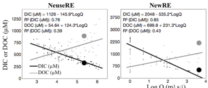
Figure 3.4 – Scatter plots of river discharge against DIC and DOC ... 66
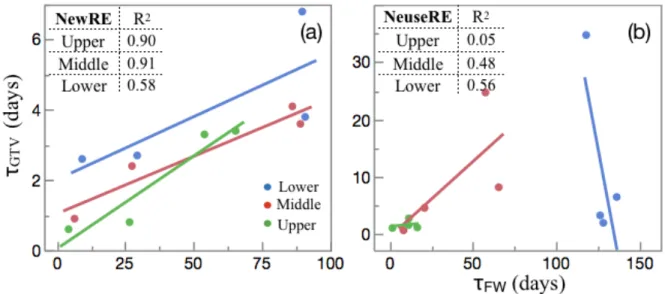
Figure 3.5 – Scatter plots of τGTV and τFW ... 69
Figure 3.6 – Bar graph of sectional mean T/N-T... 71
Figure 3.7 – Time series of sectional-mean Revelle factor ... 74
Figure 3.8 – Horizontal bar chart of storm-driven CO2 fluxes ... 77
Figure 4.1 – Site map showing the location of Lake Taihu and the Taihu Laboratory for Lake Ecosystem Research in Jiangsu Province, China ... 87
Figure 4.2 – Conceptual figure describing how 13C was partitioned between cellular and environmental pools ... 93
Figure 4.3 – Time-series plot of physical and chemical properties. ... 97
Figure 4.5 – Proportion of Chlorophyll-a represented by major phytoplankton taxa,
as a fraction of total Chlorophyll-a, and POC... 100
Figure 4.6– Relationship between pCO2 and the fraction of total chlorophyll-a represented by cyanobacteria ... 103
Figure 4.7 – Relationship between pCO2 and εp-POC. ... 104
Figure 4.8 – Linear regression of the change in ∂13CDIC and changes in DIC ... 105
Figure 4.9 – Calculated δ13Cfixed and modeled δ13Cphyto (‰) as a function of pCO2 ... 106
Figure 4.10 – Sensitivity analysis of model variables ... 107
Figure 5.1 – Literature comparison of k parameterizations for estuaries ... 122
Figure 5.2 – Site map, showing location of EC tower and in-situ sensors ... 124
Figure 5.3 – Wind rose for New River Marine Corps Air Station ... 125
Figure 5.4 – Time-series plots of pCO2, wind speed, CO2 flux, and temperature... 126
Figure 5.5 – Plot of CO2 Flux, standard deviation of CO2 flux, and count of hourly averages, placed into 10o bins of wind direction... 127
Figure 5.6 – Relationship between measured and modeled CO2 flux ... 128
Figure 5.7 – Relationship between U10 and k, showing all data, all data split by day and night, all data binned at 1.5 m s-2 intervals, and binned day and night ... 131
Figure 5.8 – Conceptual diagram of the air-water boundary layer ... 132
Figure 5.9 – Literature comparison of k parameterizations for estuaries, updated with the results of this study ... 133
LIST OF ABBREVIATIONS AND SYMBOLS
‰ Parts Per Thousand
∂ Partial Derivative
δ13C Stable Isotopic Signature of Carbon
ε Isotope Fractionation Factor
Ω Saturation State
τFW Freshwater Age
τGTV Gas Transfer Velocity Time Scale
AVP Autonomous Vertical Profiler
C Carbon
CCM Carbon Concentrating Mechanism
CH4 Methane
Chl-a Chlorophyll-a
CO2 Carbon Dioxide
CO32- Carbonate
DIC Dissolved Inorganic Carbon
DO Dissolved Oxygen
DOC Dissolved Organic Carbon
FW Fresh Water
GF/F Glass Fiber Filters
GPS Global Positioning System
HAB Harmful Algal Bloom
HCO3- Bicarbonate
k Gas Transfer Velocity
k600 Gas Transfer Velocity normalized to Sc = 600
Ko Solubility Coefficient
MBZ Minimum Buffering Zone
NeuseRE Neuse River Estuary
NewRE New River Estuary
OM Organic Matter
pCO2 Partial Pressure of Carbon Dioxide
ΔpCO2 Air-Water Concentration Gradient of Carbon Dioxide
POM Particulate Organic Matter
ppm Parts Per Million
PPR Primary Productivity
R Revelle Factor
ScSST Schmidt Number at Ambient Sea Surface Temperature
SST Sea Surface Temperature
SSS Sea Surface Salinity
TA Total Alkalinity
TDN Total Dissolved Nitrogen
TDP Total Dissolved Phosphorus
U10 Wind Speed at 10 meters elevation
x̄ Arithmetic Mean
Chapter 1
Introduction and Motivation
Across the freshwater to marine continuum, from headwater streams to estuaries, the biogeochemical fate of material is governed by the relative time scales of reaction and transport. The concentration of material within these systems is determined by the net effect of biological and geochemical consumption and production, relative to physical removal and supply. Hence, one may make qualitative inferences about the biology and ecology of a system based on the changes in chemical constituents over time. This endeavor defines chemical oceanography.
of the organic matter produced within the estuary was exported off shore. Clearly, if we are to apply these ‘open-system’ approaches to environments as dynamic as estuaries, we must better constrain the physical processes that obscure the biological and chemical signals of interest.
For estuaries, the processes altering C distributions through space and time can be broken down into a few main categories: 1) surface or subsurface inputs, 2) mixing with the coastal ocean, 3) vertical exchange with sediments, and 4) exchange with the atmosphere. Water budgets can be balanced rather simply, and sediment burial can be integrated over time using
geochronological tools. The final point, however, is perhaps the most challenging. This is
because CO2 flux is driven by the interaction of three factors: air-water concentration gradient of CO2 (ΔpCO2), gas solubility (Ko), and physical forcing which can be summarized in a ‘gas transfer velocity’ (k) (McGillis et al., 2004; Wanninkhof and McGillis, 1999). When using a ‘bulk transfer approach’ such as this, CO2 flux may be expressed as (1.1):
CO2 flux = k * Ko * ΔpCO2
(Podgrajsek et al., 2014a, Podgrajsek et al., 2014b). Each of these factors may at times challenge our ability to estimate k with acceptable precision (Raymond and Cole, 2001; Wanninkhof et al., 2009). While air-water CO2 exchange is often a small component of estuarine C budgets
(Crosswell et al., 2017; Maher and Eyre 2012), this biogeochemical flux is subject to great uncertainty, making its interpretation problematic. This problem is compounded in estuaries surrounded by wetlands (Cai and Wang, 1998; Cai et al., 1999; Cai 2011; Jeffrey et al, 2016; Laruelle et al., 2017) or experiencing large groundwater inputs (Macklin et al., 2014; Ruiz-Halpern et al., 2015; Sadat-Noori et al., 2016), both of which have been shown to significantly increase ΔpCO2. Therefore, our ability to draw quantitative inferences about the metabolic state of estuaries using a carbon budget approach is in part limited by our ability to accurately quantify air-water CO2 exchange.
Not only are estuarine CO2 emissions informative of ecosystem metabolism, they also represent a significant component of the global C cycle. Still, estimates of air-water CO2 exchange from estuaries, integrated over larger regional and global scales, have been hampered due to the high spatial and temporal variability characteristic of these systems. The first
opposite sign, of average air-water CO2 exchange over the continental shelf (Chen et al., 2013; Laruelle et al., 2013)
Global estuarine CO2 emissions are often constrained by scaling the results of individual studies that have quantified CO2 flux over a sufficiently long time period. Clearly, this approach is problematic in that it generates estimates that are biased towards frequently-studied systems. To address this problem, some have assumed that CO2 flux is a function of net ecosystem metabolism, allowing estimates of air-water CO2 exchange to be extended to estuaries where direct pCO2 measurements do not exist (Borges and Abril 2012; Laruelle et al., 2013). While precedent exists for general agreement between CO2 flux and net metabolism exists in the literature (Raymond et al., 2000; Gazeau et al., 2012; Borges and Abril 2012; Regnier et al., 2013), there is reason to expect that these factors may become uncoupled or obscured. For example, nitrifying chemoautotrophs will consume oxygen and alkalinity while oxidizing ammonium to nitrate, while also reducing pH, the net effect of which increases pCO2 (Borges and Abril 2012). In some polluted estuaries, rates of nitrification may be sufficient to consume upwards of 20-50% of DO, generating CO2 emissions (resulting from net alkalinity
consumption) far beyond what would be expected for aerobic respiration of the same oxygen demand (Berounsky and Nixon 1993; Vanderborght et al., 2002).
2008; Joesoef et al., 2015); hence, metabolism-derived CO2 fluxes will always constitute underestimates in river-dominated estuaries.
To summarize, the quantification of carbon fluxes through estuaries, including
transformations between inorganic and organic, particulate and dissolved pools, can inform our understanding of: 1) how these systems are linked with their watersheds, 2) relative rates of net ecosystem metabolism, and 3) the role of these systems in the larger global C cycle. The least constrained term in many estuarine C budgets is air-water CO2 exchange, and the magnitude of this flux has relevance to the global carbon cycle. Hence, it is critical that we better characterize the spatial and temporal variability in estuarine CO2 emissions, and better understand the factors that drive this variability. Addressing this research gap is the focus of the next two chapters of this dissertation.
In chapter 2, an unprecedented dataset consisting of two consecutive years of high-resolution pCO2 surveys are used to investigate watershed-scale drivers of air-water CO2
exchange in a set of North Carolina estuaries. An argument is presented that freshwater residence time, which modulates supplies of nutrients and organic carbons, as well as phytoplankton
flushing, is a universal driver of pCO2 dynamics across estuarine morphologies. Chapter 3
grounded in stable isotope geochemistry is combined with a simple model to ask whether the intense CO2 limitation associated with dense harmful algal blooms (HABs) promotes the dominance of cyanobacteria. Finally, in chapter 5, we combine surface-water pCO2 measurements with eddy covariance measurements of CO2 flux in an effort to refine our understanding of the various physical drivers on air-water gas transfer in estuaries.
REFERENCES
Abril, G., Commarieu, M. V., Sottolichio, A., Bretel, P., & Guérin, F. (2009). Turbidity limits gas exchange in a large macrotidal estuary. Estuarine, Coastal and Shelf Science, 83(3), 342–348. https://doi.org/10.1016/j.ecss.2009.03.006
Berounsky, V. M., & Nixon, S. W. (1993). Rates of Nitrification along an Estuarine Gradient in Narragansett Bay. Estuaries, 16(4), 718. https://doi.org/10.2307/1352430
Borges, A. V., Vanderborght, J.-P., Schiettecatte, L., Gazeau, F., Ferron-Smith, S., Delille, B., & Frankignoulle, M. (2004). Variability of the Gas Transfer Velocity of CO2 in a Macrotidal Estuary (the Scheldt). Estuaries, 0(4), 593–603.
Borges, A. V. (2005). Do We Have Enough Pieces of the Jigsaw to Integrate CO2 Fluxes in the Coastal Ocean? Estuaries, 28(1), 3–27.
Borges, A. V., & Abril, G. (2012). Carbon Dioxide and Methane Dynamics in Estuaries. Treatise on Estuarine and Coastal Science (Vol. 5). Treatise on Estuarine and Coastal Science, 119-161. https://doi.org/10.1016/B978-0-12-374711-2.00504-0
Cai, W.-J., & Wang, Y. (1998). The chemistry, fluxes, and sources of carbon dioxide in the estuarine waters of the Satilla and Altamaha Rivers, Georgia. Limnology and
Oceanography, 43, 657–668.
Cai, W.-J., Pomeroy, L. R., Moran, M. A., & Wang, Y. (1999). Oxygen and carbon dioxide mass balance for the estuarine-intertidal marsh complex of five rivers in the Southeastern U.S. Limnology and Oceanography, 44(3), 639–649. https://doi.org/10.4319/lo.1999.44.3.0639 Cai, W.-J. (2011). Estuarine and Coastal Ocean Carbon Paradox: CO2 Sinks or Sites of
Terrestrial Carbon Incineration? Annual Review of Marine Science, 3(1), 123–145. https://doi.org/10.1146/annurev-marine-120709-142723
Chen, C. T. a, Huang, T. H., Chen, Y. C., Bai, Y., He, X., & Kang, Y. (2013). Air-sea exchanges of CO2 in the world’s coastal seas. Biogeosciences, 10, 6509–6544.
https://doi.org/10.5194/bg-10-6509-2013
Crosswell, J. R., Anderson, I. C., Stanhope, J. W., Van Dam, B., Brush, M. J., Ensign, S., … Paerl, H. W. (2017). Carbon budget of a shallow, lagoonal estuary: Transformations and source-sink dynamics along the river-estuary-ocean continuum. Limnology and
Oceanography. 62: S29–S45. https://doi.org/10.1002/lno.10631
Gazeau, F., Gattuso, J., Middelburg, J. J., Brion, N., Schiettecatte, S., Frankignoulle, M., & Borges, A. V. (2012). Planktonic and Whole System Metabolism in a Nutrient-rich (the Scheldt Estuary) Estuary. Estuaries, 28(6), 868–883.
Ho, D. T., Ferrón, S., Engel, V. C., Larsen, L. G., & Barr, J. G. (2014). Air-water gas exchange and CO2 flux in a mangrove-dominated estuary. Geophysical Research Letters, 41(1), 108– 113. https://doi.org/10.1002/2013GL058785
Jeffrey, L. C., Maher, D. T., Santos, I. R., McMahon, A., & Tait, D. R. (2016). Groundwater, Acid and Carbon Dioxide Dynamics Along a Coastal Wetland, Lake and Estuary
Continuum. Estuaries and Coasts, 39(5), 1325–1344. https://doi.org/10.1007/s12237-016-0099-8
Jiang, L.-Q., Cai, W.-J., & Wang, Y. (2008). A Comparative Study of Carbon Dioxide Degassing in River- and Marine-Dominated Estuaries. Limnology and Oceanography, 53(6), 2603–2625.
Joesoef, A., Huang, W. J., Gao, Y., & Cai, W.-J. (2015). Air-water fluxes and sources of carbon dioxide in the Delaware Estuary: Spatial and seasonal variability. Biogeosciences, 12(20), 6085–6101. https://doi.org/10.5194/bg-12-6085-2015
Kemp, W.M., Boynton, W.R. (1980). Influence of biological and physical processes on dissolved oxygen dynamics in an estuarine system: Implications for measurement of community metabolism. Estuarine and Coastal Marine Science. 11(4), 407-431.
https://doi.org/10.1016/S0302-3524(80)80065-X
Laruelle, G. G., Dürr, H. H., Lauerwald, R., Hartmann, J., Slomp, C. P., Goossens, N., & Regnier, P. a G. (2013). Global multi-scale segmentation of continental and coastal waters from the watersheds to the continental margins. Hydrology and Earth System Sciences, 17, 2029–2051. https://doi.org/10.5194/hess-17-2029-2013
Laruelle, G. G., Landschützer, P., Gruber, N., Tison, J.-L., Delille, B., & Regnier, P. (2017). Global high resolution monthly pCO2 climatology for the coastal ocean derived from neural network interpolation. Biogeosciences Discussions, (2014), 1–40.
https://doi.org/10.5194/bg-2017-64
Macklin, P. a., Maher, D. T., & Santos, I. R. (2014). Estuarine canal estate waters: Hotspots of CO2 outgassing driven by enhanced groundwater discharge? Marine Chemistry, 167, 82–92. https://doi.org/10.1016/j.marchem.2014.08.002
McGillis, W. R., Edson, J. B., Zappa, C. J., Ware, J. D., McKenna, S. P., Terray, E. A., … Feely, R. A. (2004). Air-sea CO2 exchange in the equatorial Pacific. Journal of Geophysical Research C: Oceans, 109(8), 1–17. https://doi.org/10.1029/2003JC002256
Mørk, E. T., Sørensen, L. L., Jensen, B., & Sejr, M. K. (2014). Air–Sea CO2 Gas Transfer Velocity in a Shallow Estuary. Boundary-Layer Meteorology, 151(1), 119–138. https://doi.org/10.1007/s10546-013-9869-z
Nixon, S. W. and Oviatt, C. A. (1972). Preliminary Measurements of Midsummer Metabolism in Beds of Eelgrass, Zostera Marina. Ecology, 53, 150–153. doi:10.2307/1935721
Nixon, S.W., Granger, S.L. & Nowicki, B.L. (1995). An assessment of the annual mass balance of carbon, nitrogen, and phosphorus in Narragansett Bay. Biogeochemistry 31.
https://doi.org/10.1007/BF00000805
Odum, H. T., Monographs, S. E., Jan, N., & Odum, H. T. (1957). Trophic Structure and Productivity of Silver Springs, Florida. Ecological Society of America, 27(1), 55–112. Odum, H. T. (1956). Primary production in flowing waters. Limnology and Oceanography, 1(2),
102–117. https://doi.org/10.4319/lo.1956.1.2.0102
Owens, M., & Edwards, R. (1962). The Effects of Plants on River Conditions: III. Crop Studies and Estimates of Net Productivity of Macrophytes in Four Streams in Southern
England. Journal of Ecology,50(1), 157-162. doi:10.2307/2257200
Podgrajsek, E., Sahlée, E., Bastviken, D., Holst, J., Lindroth, A., Tranvik, L., & Rutgersson, A. (2014a). Comparison of floating chamber and eddy covariance measurements of lake greenhouse gas fluxes. Biogeosciences, 11(15), 4225–4233. https://doi.org/10.5194/bg-11-4225-2014
Podgrajsek, E., Sahlée, E., & Rutgersson, A. (2014b). Diel cycle of lake-air CO2 flux from a shallow lake and the impact of waterside convection on the transfer velocity. Journal of Geophysical Research: Biogeosciences, 119, 487–507.
https://doi.org/10.1002/2013JG002552.Received
Raymond, P. a., Bauer, J. E., & Cole, J. J. (2000). Atmospheric CO2 evasion, dissolved inorganic carbon production, and net heterotrophy in the York River estuary. Limnology and
Oceanography, 45(8), 1707–1717. https://doi.org/10.4319/lo.2000.45.8.1707
Raymond, P. A., & Cole, J. J. (2001). Gas Exchange in Rivers and Estuaries: Choosing a Gas Transfer Velocity. Estuaries, 24(2), 312–317.
Ruiz-Halpern, S., Maher, D. T., Santos, I. R., & Eyre, B. D. (2015). High CO2 evasion during floods in an Australian subtropical estuary downstream from a modified acidic floodplain wetland. Limnology and Oceanography, 60, 42–56. https://doi.org/10.1002/lno.10004 Sadat-Noori, M., Maher, D. T., & Santos, I. R. (2016). Groundwater discharge as a source of
dissolved carbon and greenhouse gases in a subtropical estuary. Estuaries and Coasts, 39(3), 639–656. https://doi.org/10.1007/s12237-015-0042-4
Upstill-Goddard, R. C. (2006). Air–sea gas exchange in the coastal zone. Estuarine, Coastal and Shelf Science, 70(3), 388–404. https://doi.org/10.1016/j.ecss.2006.05.043
Vanderborght, J., Wollast, R., Loijens, M., & Regnier, P. (2002). Application of a Transport-Reaction Model to the Estimation of Biogas Fluxes in the Scheldt Estuary.
Biogeochemistry, 59, 207-237. Retrieved from http://www.jstor.org/stable/1469912 Wanninkhof, R., & Mcgillis, W. R. (1999). A cubic relationship between air-sea CO2 exchange
and wind speed. Geophysical Research Letters, 26(13), 1889–1892.
Wanninkhof, R., Asher, W. E., Ho, D. T., Sweeney, C., & McGillis, W. R. (2009). Advances in Quantifying Air-Sea Gas Exchange and Environmental Forcing. Annual Review of Marine Science, 1(1), 213–244. https://doi.org/10.1146/annurev.marine.010908.163742
Zappa, C. J., McGillis, W. R., Raymond, P. A., Edson, J. B., Hintsa, E. J., Zemmelink, H. J., Dacey, J. W. H., & Ho, D.T. (2007). Environmental turbulent mixing controls on air-water gas exchange in marine and aquatic systems. Geophys. Res. Lett., 34, L10601,
Chapter 2
Watershed-scale drivers of air-water CO2 exchanges in two lagoonal, North Carolina (USA) estuaries1
2.1. Introduction
Estuaries are important biogeochemical and trophic links between terrestrial and marine systems, and provide critical ecosystem services to coastal populations (Hobbie, 2000;
Pendleton, 2008; Wetz and Yoskowitz, 2013). Estuaries often receive large allochthonous organic matter loads, which support high remineralization rates and drive them towards net ecosystem heterotrophy and CO2 degassing (Frankignoulle et al. 1998; Cai 2011; Borges and Abril 2011; Bauer et al. 2013). At the same time, nutrients (nitrogen and phosphorus) supplied externally or recycled internally drive high rates of autochthonous organic matter production in these ecosystems, causing some estuaries to act as CO2 sinks (Crosswell et al, 2012; Crosswell et al, 2017; Drupp et al, 2011; Hunt et al, 2011; Maher and Eyre, 2012). The balance between these factors varies over space and time, making it difficult to globally integrate CO2 fluxes across these diverse ecosystems. Early attempts at scaling estuarine CO2 fluxes globally or regionally resulted in relatively high estimates, on the order of 100-500 mmol C m2 d-1 (Frankignoulle et al. 1998; Borges et al. 2004a, 2005), which have since been revised downward by an order of
1 This Chapter previously appeared as an article in the Journal of Geophysical Research: Biogeosciences. The original citation is as follows:
Van Dam, B., Crosswell, J. R., Anderson, I. C., and H.W. Paerl. (2018), Watershed-scale drivers of air-water CO2 exchanges in two lagoonal, North Carolina (USA) estuaries. Journal of
magnitude (Chen and Borges 2009; Laruelle et al. 2010, 2013; Cai 2011; Maher and Eyre 2012; Regnier et al. 2013). This decrease was largely due to the inclusion of microtidal and marine-dominated systems, which are relatively small sources of CO2 to the atmosphere (Jiang et al. 2008), and as a result, the most recent globally scaled estimates of estuarine CO2 degassing have again decreased, to ~20-40 mmol C m2 d-1 (Maher and Eyre 2012; Laruelle et al. 2013; Regnier et al. 2013). Because microtidal, lagoonal estuaries make up ~50% of the global estuarine surface area (Kennish and Paerl 2010; Crosswell et al. 2012; Chen et al. 2013; Laruelle et al. 2013), information on the drivers of air-water CO2 exchange across the diverse range of such systems is needed if we are to accurately scale this biogeochemical flux globally.
In microtidal, lagoonal estuaries, variations in the timing and magnitude of river
(Langley and Megonigal 2010; Mozdzer and Megonigal 2012), and the invasion of this
anthropogenic CO2 into the coastal ocean may increase seagrass production (Zimmerman et al. 2015). Hu and Cai (2013) demonstrated that acidification (due to anthropogenic CO2 emissions and eutrophication) was greater for estuaries receiving lower loads of HCO3- and other
weathering products from their respective rivers. A subsequent analysis reinforced this concept by showing that a majority of Texas estuaries are experiencing long-term acidification, driven largely by reduced alkalinity loads stemming from drought and human water use (Hu et al. 2015). The potential for acidification in estuaries not experiencing drought has received less attention, despite the fact that acidification may have particularly severe impacts on the economies of communities surrounding these estuaries (Ekstrom et al. 2015). Recent studies have indicated that estuaries receiving moderate or low alkalinity loads from their tributary rivers (like those of eastern North Carolina) may be particularly vulnerable to acidification due to mixing with ocean waters high in dissolved CO2, as well as those receiving inputs of acidity through aerobic (Hu and Cai 2013) and anaerobic pathways (Cai et al., 2017). Therefore, knowledge of how carbonate buffering varies between estuaries experiencing the same climatic conditions but different riverine end-member chemistries is critical if we are to predict how coastal systems will respond to future acidification.
Ruiz-Halpern et al. 2015). Both episodic and seasonal variations in river discharge, strongly affect air-water CO2 exchange in estuaries (Cai 2011; Borges and Abril 2012; Bauer et al. 2013; Chen et al. 2013); however, quantitative relationships between estuarine C cycling and catchment hydrology remain relatively poorly defined.
2.2. Materials and Methods
2.2.1 Study Site
The Neuse River flows from the urbanized North Carolina Piedmont in the Raleigh-Durham-Chapel Hill Triangle area through the coastal plain, towards its terminus in Pamlico Sound; the third largest estuarine system in North America (~7,770 km2; Figure 2.1). The NeuseRE begins near New Bern, NC, where the funnel-shaped estuary widens considerably and oligohaline conditions prevail. Due to restricted exchange across the narrow inlets of Pamlico Sound, astronomical tides are minimal (<10 cm); lateral and longitudinal water movements are mostly driven by meteorological factors like wind and fresh water discharge (Luettich et al. 2000), hence, we consider this estuary to be ‘river-dominated’. Submarine groundwater discharge to the estuary is small relative to inputs of water and nutrients from the Neuse and Trent rivers (Fear et al. 2007; Null et al. 2011). This system has been well studied for decades via long term monitoring projects like the Neuse River Estuary Modeling and Monitoring
Figure 2.1. (a) General site map showing the locations of the NewRE and NeuseRE, their respective watersheds (dark grey), and USGS stream flow gauges (black triangles) for which river discharge measurements were obtained. Detailed maps of the NewRE (b) and NeuseRE (c) showing the location of meteorological stations (black squares), autonomous vertical profilers (AVPs, hollow squares), discrete sampling stations (black circles), and dataflow cruise track (dashed line).
The New River is a small coastal plain river, located entirely in Onslow County, NC, USA. Agricultural land use dominates its watershed, which is approximately one-tenth the size of the Neuse River watershed. The upper estuary is surrounded by the city of Jacksonville, NC, with a 2010 census population of over 70,000 (Figure 2.1). Impervious surfaces, along with the small size of the watershed, cause river inputs to the NewRE to be relatively “flashy”, with discharge quickly peaking and receding after storms (Peierls et al. 2012). Because of relatively
-Piney Green Jacksonville -77.3° -77.4° -77.5° 34.7° 34.6° -76.5° -77° 35.3° 35° Cary Durham Raleigh Charlotte High Point Greensboro Fayetteville -75° -76° -77° -78° -79° -80° -81° 36° 35°0 55 110
km
0 2.5 5
km 0 5 10km
¯
S Autonomous Vertical Profiler
-
Cruise Track! Sample Stations
low river discharge, and long residence time, we consider this estuary to exemplify ‘marine-dominated’ traits. Before transitioning into the oligohaline NewRE near Jacksonville, NC, the New River enters a relatively short (~12 km) tidal freshwater reach, where N loads are attenuated by denitrification in the surrounding forested wetlands (Ensign et al. 2013; Von Korff et al. 2014). The body of the NewRE consists of 5 interconnected lagoons of differing sizes. The seaward lagoon is connected to the Atlantic Ocean by a narrow inlet that limits oceanic exchange. The tidal amplitude is correspondingly low, ranging from approximately 0.25 m in middle and upper segments to nearly 1 m at the New River Inlet. This low tidal amplitude, along with freshwater discharge, drives vertical stratification and frequent bottom water hypoxia, as often occurs in the NeuseRE. Following upgrades to a sewage treatment plant in 1998, primary production in the NewRE decreased, causing a transition from eutrophic (250-500 gC m-2y-1) to mesotrophic status (<250 gC m-2y-1) (Anderson, personal comm.; Mallin et al. 2005). Fringing marshes are present in both estuaries, but constitute a relatively small fraction of the intertidal area; salt marshes and swamps represent approximately 21 and 6% of the shoreline in the NewRE (Currin et al. 2015).
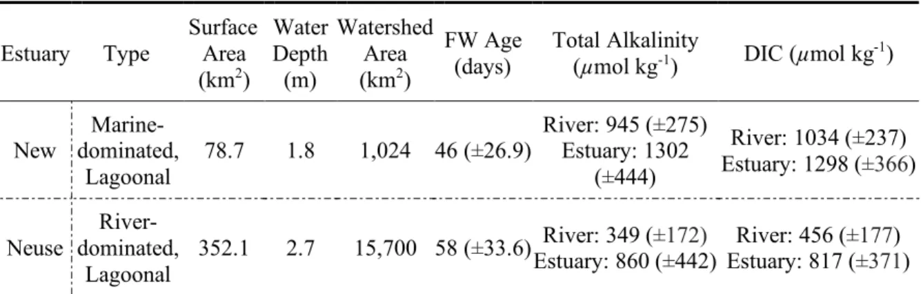
Table 2.1. Site description, average physical and chemical properties. Standard deviations are shown in parentheses.
Estuary Type
Surface Area (km2)
Water Depth (m)
Watershed Area (km2)
FW Age (days)
Total Alkalinity
(µmol kg-1) DIC (µmol kg-1)
New dominated, Marine-Lagoonal
78.7 1.8 1,024 46 (±26.9) River: 945 (Estuary: 1302 ±275) (±444)
River: 1034 (±237) Estuary: 1298 (±366)
Neuse
River-dominated,
Lagoonal
2.2.2 Synoptic Surveys
From October 2014 to October 2016, 74 high-resolution surveys of surface water partial pressure CO2 (pCO2) were conducted at bi-weekly to monthly intervals, 36 in the NeuseRE and 38 in the NewRE. 21 of the NewRE surveys were conducted as a part of a study investigating diel pCO2 variability, during which 3 consecutive surveys were completed in a contiguous 25-hour period, at dawn of the first day, dusk of the first day, and dawn of the following day. For the purposes of general comparisons in this study, these dawn-dusk-dawn surveys were combined into 7 representative daily averages. All other surveys began in the mid-morning (08:30-10:00 AM). The choice of a mid-morning sampling time may lead to a small over-estimation of pCO2 due to diurnal variations, but has been used extensively because it is close to the idealized midpoint between dawn pCO2 maxima and dusk pCO2 minima (Crosswell et al. 2012; Maher and Eyre 2012). For the purpose of this inter-estuary comparison, CO2 fluxes were estimated from longitudinal transects alone, which covered slightly different regions of each estuary. Because of the small size of the NewRE, a wide salinity range (~5 - 35) was surveyed during each transect. The surface area of the NeuseRE is ~4 times greater than the NewRE; thus, fixed stations covered a smaller section of the salinity range in this system (0 - ~20). The NeuseRE becomes strongly influenced by other watersheds (i.e. Tar-Pamlico) beyond the downstream extent of the lowest estuarine segment (Figure 2.1).
2.2.3 CO2 Flux Determinations
NeuseRE (Crosswell et al. 2012) and NewRE (Crosswell et al, 2017). In situ pCO2 was measured using a combined laminar flow shower-head equilibrator and infrared detector (LI-COR, Li-840A). Analyzers of this type have been deployed extensively in previous studies (Frankignoulle and Borges 2002; Wang and Cai 2004; Zhai et al. 2005; Crosswell et al. 2012, 2014, 2017; Santos et al. 2012). Water was continuously pumped from a depth of approximately 0.5 m (variable with boat speed) into a shower-head equilibrator, and air was circulated between this equilibrator and the infrared analyzer. Water was also sent through a flow-thru cell (Dataflow) for measurements of chlorophyll-a fluorescence (chl-a), dissolved oxygen (DO), pH, salinity, temperature, and turbidity (YSI 6600 multiparameter sonde, Yellow Springs Inc, Yellow
Springs, OH). Measurements were recorded at 0.5 hz, corresponding to a spatial resolution of ~6 m at a boat speed of ~40 km h-1. The raw CO2 mixing ratio in the equilibrator (xCO2) was
calibrated against 2-3 standards, ranging from 100-5000 ppm (certified to ± 2%), before and after each cruise, when measurements of atmospheric pCO2 (pCO2(air)) were also made. This
calibration curve was extrapolated linearly for xCO2 beyond 5000 µatm. pCO2(water) was calculated from calibrated xCO2 in the equilibrator according to equation (2.1), where Tw and TSHE are measured temperatures in the water and equilibrator respectively (Takahashi et al., 1993).
𝑝𝐶𝑂$(&'()*)= 𝑥𝐶𝑂$∗ 𝑒(0.02$3 × [7897:;<]) (2.1)
calculate CO2 flux (mmol C cm2 hr-1) using the stagnant-layer model (Smethie et al. 1985) according to equation (2.2):
𝑓𝑙𝑢𝑥 = 𝑘 ∗ 𝐾C ∗ ∆𝑝𝐶𝑂$ (2.2)
where ∆pCO2 is the air-water pCO2 gradient. By convention, a positive ∆pCO2 indicates pCO2(water) greater than pCO2(air). Ko is the CO2 solubility coefficient (Weiss 1974). The gas transfer velocity, k (cm h-1) was calculated using the following equation from Jiang et al. (2008):
𝑘 = EF0.314 ∗ 𝑈L0$− 0.436 ∗ 𝑈L0+ 3.99Q ∗ (𝑆𝑐TT7/600)V90.W (2.3) where U10(m s-1) is the daily averaged wind speed normalized to a height of 10m. A brief discussion of the limitations of this method, including a sensitivity analysis of CO2 flux using different k parameterizations, is included in the supporting information (Figure A1). Briefly, the use of different k parameterizations may over- or underestimate CO2 flux by a factor of ~1.6-2 (Table A1). However, we chose the parameterization of Jiang et al. (2008) because it constitutes an intermediate estimate of k, considers both marine- and river-dominated estuaries, and is consistent with previous studies in both the NeuseRE (Crosswell et al., 2012) and NewRE
(Crosswell et al., 2017). Hourly average wind speed was obtained from two autonomous vertical profilers deployed in the NewRE (Reynolds-Fleming et al. 2002), and from two meteorological stations (KEWN and KNKT) near the NeuseRE (Figure 2.1). For each estuarine segment, wind speed from the closest meteorological station was averaged for each day, and applied to daily-average ∆pCO2 with equations 2.2 and 2.3. ScSSTis the Schmidt number for CO2 at ambient sea-surface temperature (SST) and sea-sea-surface salinity (SSS). Because sampling began near the middle of 2014, study-years rather than calendar years were used to calculate annual fluxes (Year 1: Oct 27, 2014 to Oct 26, 2015. Year 2: Oct 27, 2015 to Oct 16, 2016).
collected with a diaphragm pump at the surface and ~0.5 m from the bottom, stored in a refrigerator unpreserved with no headspace in 20 mL scintillation vials, and analyzed on a Shimadzu TOC-5000A within 24 hours. Previous studies have shown a difference between DIC in preserved and unpreserved samples (Crosswell et al. 2012); however, this difference is small relative to observed spatial and temporal variability in DIC. Hence, no correction was applied to DIC values here. CO2sys (Lewis and Wallace, 1998) was used to calculate all additional
carbonate system parameters, including Total Alkalinity (TA) and Revelle Factor (R). Carbonic acid dissociation constants (K1 and K2) of Dickson and Millero, (1987) were assumed, and the NBS scale was used for pH. Measured pCO2, DIC, SST, and SSS were used as CO2sys inputs. pCO2 measurements were only used when the boat was stationary for a sufficient time (at least 10 minutes) to ensure system equilibration with the parcel of water being sampled for DIC, temperature, and salinity.
Non-linear changes in pCO2 occur when mixing or net biological processes alter the concentration of DIC, and these changes are buffered to an extent that is determined by the relative concentrations of TA and DIC. Because both TA and DIC vary across the estuary, this carbonate buffering also exhibits spatial and temporal variability. Previous studies have shown the presence of a minimum buffering zone (MBZ) in mesohaline portions of some tropical and subtropical estuaries (Hu and Cai, 2013; Ruiz-Halpern et al. 2015, Jeffrey et al. 2016). At this MBZ, when temperature and salinity are held constant, pCO2 is most sensitive to additional inputs of DIC. Here, pH is approximately half way between the pK1 and pK2 of H2CO3 (Cai et al. 2011), the ratio of DIC : TA approaches unity, and the Revelle Factor is maximized. The Revelle Factor (R) is a commonly used buffer factor of the carbonate system, defined as:
𝑅 =∂𝑝CO$ ∂DIC ×
and is implicitly related to the ratio of DIC : TA (Egleston et al. 2010). In this study, we calculate R in CO2sys (Lewis and Wallace, 1998) using paired measurements of DIC, pCO2, SST, and SSS. While the carbonate system can be quantitatively assessed using other sets of paired observations (DIC and TA, pCO2 and pH, etc.), the combination of DIC and pCO2 is preferred, given the current uncertainty in carbonate system measurements (Millero 2013). We assess spatial and temporal variations in R, and discuss them in the context of riverine TA and DIC inputs and ocean acidification.
2.2.4 Freshwater Age
A variety of metrics are used to assess the flow of C (and other properties) through ecological systems and the time scales involved, known as ‘system diagnostic times’ (Sierra et al. 2017). In estuaries, terms like residence time, transit time, and age are often used, but their calculation often requires assumptions of steady state or homogeneous mixing, which are often not met (Alber and Sheldon 1999). A lag-time exists for water flowing between the head and mouth of all estuaries, meaning that the time for a given particle to exit the system varies along its length. Additionally, river flow can change rapidly, and if water residence time is to be calculated as the ratio of estuarine volume to river discharge, then the averaging time interval for discharge must be appropriate.
by the ratio of total to gauged watershed (0.22 and 0.69 for the NewRE and NeuseRE
respectively) (Ensign et al. 2004; Peierls et al. 2012). The time period over which river discharge was averaged was then calculated using the ‘date-specific’ method of Alber and Sheldon, 1999 (Peierls et al. 2012). This method provides a robust estimate of the amount of time needed for river discharge to replace the volume of fresh water in the estuary. FW age for each estuarine segment was calculated as a cumulative sum, including all upstream segments.
2.2.5 Estuarine vs Riverine contributions to CO2
Allochthonous, river-borne CO2 is released to the atmosphere in estuaries, but it is also replenished when riverine OC is respired to CO2 in estuaries. The balance between these autochthonous and allochthonous contributions to CO2 degassing is difficult to discern, and likely varies in estuaries ranging from river-dominated, like the NeuseRE, to marine-dominated systems like the NewRE. We estimated the relative contributions of river-borne and estuarine CO2 sources ([CO2]river and [CO2]estuary) for both the river-dominated NeuseRE and the marine-dominated NewRE using methods adapted from Jiang et al (2008) and Joesoef et al (2015). In essence, CO2 delivered by the river was balanced against losses due to air-water exchange (integrated over the cumulative FW age), with the remainder attributed to net estuarine production.
First, for each segment and sampling date, the contribution of DIC due to mixing with ocean water (DICmixing w/O) was calculated using equation (2.4):
where Si and Socean are the average salinities for each estuarine segment, and the ocean (35) respectively, while DICocean is the DIC concentration of the oceanic end-member (2000 umol kg -1). The remaining DIC was attributed to mixing with river water (DICmixing w/R):
DICmixing w/R = DICmixing w/O + DICriver * (1- Si/Socean), (2.5) where DICriver is the measured or modeled DIC concentration of river water for that date. DICriver in the NewRE was estimated as the 0 salinity end-member for each date using a linear regression of measured estuarine DIC and salinity. An implied assumption of linear mixing may add a small uncertainty to subsequent calculations. DICriver in the Neuse was measured, so it was not
necessary to model this value. Both of these calculations were repeated for TA (oceanic end-member was assumed to be 2200 umol kg-1), allowing both CO2 contributions from mixing with river water and the ocean ([CO2]mixing w/R, and [CO2]mixing w/O respectively) to be calculated with DIC, TA, and a T and S dependent equation of solubility (Weiss 1974). The direct CO2
contribution from riverine DIC and TA loading ([CO2]river) was then calculated as:
[CO2]river = [CO2]mixing w/R - [CO2]mixing w/O. (2.6) The concentration of CO2 produced within the estuary ([CO2]estuary) was then assumed to be equivalent to the difference between the measured [CO2] and [CO2]mixing w/R, accounting for losses due to air-water CO2 exchange, according to equation (2.7):
implicit assumption with the approach described in equation 2.7 is that shoals constitute most of the surface area of each estuarine segment, and are vertically well-mixed.
2.3. Results
2.3.1 Physicochemical and Biological Setting
Segment-average salinity ranged from <5 to 34 in the NewRE, but never exceeded 17 in the NeuseRE (Figure 2.2a, 2.2b). Seasonal trends, however, were very similar. High salinity in summer gave way to fresher conditions during the winter and spring, when precipitation in the watershed exceeded evapotranspiration (Litaker et al. 2002; Paerl et al. 2014). In the winter of 2015, maximum salinity in the NeuseRE was below the minimum salinity in the NewRE.
Chlorophyll-a (in-situ fluorescence) was generally low (< 10 µg L-1), but episodic phytoplankton blooms were associated with elevated chlorophyll-a (up to 150 µg L-1) in the late fall/early winter of both 2014 and 2015. Blooms were often restricted to the upper or middle regions of the estuary where they contributed to elevated DO, and pH as high as 9.4 and 10.7 (mid-day
Figure 2.2. Contour plots showing longitudinal transects (vertical axis) through time (horizontal axis) for both the (a) NeuseRE and (b) NewRE constructed using a linear interpolation method. The approximate timing of pCO2 surveys are indicated as the black triangles along the horizontal axis. Because the longitudinal axis of the NewRE is oriented in the north-south direction,
Latitude (decimal degrees) is used to represent distance down this estuary. Distance along the east-west oriented NeuseRE is represented with Longitude (decimal degrees). Temperature (oC), salinity, pH, chlorophyll-a (µg L-1), dissolved oxygen (mg L-1), and ∆pCO2 (µatm) are shown as the respective color axes.
2.3.2 Spatial pCO2 Trends
In general, pCO2 decreased from the river towards the ocean, a trend that was most pronounced in the NeuseRE, where air water pCO2 gradients (∆pCO2) often transitioned from positive to negative along the estuarine salinity gradient (Figure 2.2). Rapid increases in ∆pCO2 below a salinity of 5 occurred irrespective of season or discharge condition in the NeuseRE (Figure 2.3). This trend is less evident in the NewRE, occurring nearly exclusively in the fall during high discharge conditions. The highest measured ∆pCO2 values occurred in the upper estuary, with segment-average ∆pCO2 reaching 4654 (range = 3310 – 5806 µatm) and 3480
µatm (range = 3303 – 5112 µatm) in the upper NeuseRE (Sept. 2016) and NewRE (Oct. 2015) respectively. These large pCO2 super-saturation events corresponded with the lowest segment-average DO in both the NewRE (5.56 mg L-1) and the NeuseRE (5.56 mg L-1). Extreme CO2 under-saturation was observed during the phytoplankton bloom in the Winter/Spring of 2015, with lowest segment-average pCO2 of 99 in the middle NewRE, corresponding with relatively high DO (10.63 mg L-1). The lowest pCO2 was in the spring of 2016, at 72 µatm in the middle NeuseRE, also corresponding with elevated DO (11.69 mg L-1).
While Figure 2.3 shows that ∆pCO2 and salinity were generally negatively related, there was a high degree of variability in the relationship. Instances of positive and negative ∆pCO2 can be found during all seasons and all discharge regimes, across the estuarine salinity range.
to low pCO2 conditions during the winter and spring can be observed. The highly variable relationship between ∆pCO2 and salinity (Figure 2.3), as well as the ‘patchy’ nature of pCO2 distributions on any given date (Figure 2.2) suggests that biological production and consumption are important drivers of pCO2 in these shallow estuaries. The observed co-variation in CO2 and DO, occurring across all estuarine segments (Figure 2.2), supports the idea that regional
variations in biological activity (photosynthesis and respiration) drive CO2 distributions, irrespective of location along the salinity gradient.
2.3.3 Air-Water CO2 Flux
System averaged ∆pCO2 in both the NewRE and NeuseRE was generally positive (Figure 2.2); thus, both estuaries were most often sources of CO2 to the atmosphere. Two major
degassing events were seen in the fall of 2015 and 2016, both associated with the impact of large tropical weather systems, Hurricanes Joaquin and Matthew respectively. Despite most of the estuarine surface area being at or near saturation with respect to the atmosphere (Figure 2.2), high pCO2 in the upper segments generally maintained a positive air-water CO2 exchange, particularly when river discharge was high, during the fall months (Figures 2.3 and S4). Between years 1 and 2, annual average CO2 flux increased from 15.7 to 16.9 mmol C m2 d-1 in the NewRE (an 8% increase), and from 7.7 to 17.5 mmol C m2 d-1 (127% increase) in the NeuseRE. These enhanced CO2 fluxes coincided with 27 and 32% increases in river discharge from year 1 to 2 for the Neuse and New Rivers respectively (Table 2.2). Over the two-year study period, discharge was 180% of the antecedent 10-year average for the NewRE, 153% for the NeuseRE.
Table 2.2. Air-water CO2 flux as seasonal and annual averages (mmol C m2 d-1). Values in parenthesis are previous estimates from the NeuseRE (Crosswell et al. 2012) or standard deviations of segment-average salinity.
New River Estuary Neuse River Estuary
Upper Middle Lower Total Upper Middle Lower Total
Surface Area (km2) 28 38 12 79 22 100 230 352
Average Salinity (± Std. Dev.)
10.6
(4.5)
15.6
(4.2)
26.7
Winter 4.4 -6.6 -4.6 -2.37 82.6 (100) 20.1 (37.9) 3.7 (-22.0) 13.3 (2.6) Spring 9.9 16.2 7.7 12.6 90.2 (29.1) -2.7 (-2.4) 2.3 (2.8) 6.35 (2.96) Summer 9.8 3.9 6.2 6.5 59.6 (22.3) 10.2 (-3.8) 0.9 (-0.5) 7.2 (-0.02)
Fall 98.4 34.1 6.2 52.7 98.4 (115) 35.5 (55.3) 12.7 (13.9) (31.96) 24.5
Year 1 25.2 12.1 5.5 15.7 77.9 8.2 0.7 7.7
Year 2 32.2 10.4 2.4 16.9 86.7 22.6 8.8 17.5
Total 28.6 11.3 4.0 16.3 82.2 (66.6) 15.3 (21.8) 4.7 (-1.4) 12.5 (9.38)
2.3.4 Freshwater Age
During the two-year study period, FW age ranged from 6.9 to 136 days in the NeuseRE (x̄=58), and from 9.1 to 91 days in the NewRE (x̄=46) (Figure A2). Generally, FW age was low in the winter (x̄=29 and 27 days in the NewRE and NeuseRE respectively), and increased through the spring to a summer maximum of ~3 months (x̄=71 and 84 days in the NewRE and NeuseRE respectively). Storm events in the mid to late fall resulted in the lowest calculated FW ages. Minimum FW ages were observed at the end of the study, when 15-46 cm of rain fell on eastern NC during Hurricane Matthew, causing FW age to drop as low as 7 to 9 days. Between years 1 and 2, annual average FW age decreased from 66 to 54 days in the NeuseRE and from 47 to 45 days in the NewRE, consistent with increases in freshwater discharge.
2.3.5 Riverine vs Autochthonous CO2
during the spring and fall, when river discharge and ∆pCO2 were high (Figure 2.3). For systems with similar watershed characteristics and climatology, [CO2]river should scale with the ratio of watershed : estuary surface area. This ratio is 4x greater for the NeuseRE than for the NewRE (Table 2.1), offering a partial explanation for the consistently larger [CO2]river in the NeuseRE. [CO2]river was above zero along the length of both estuaries, and decreased towards the ocean.
Figure 2.4. Estuarine (red bar) and river-borne (blue) CO2 sources (mM), as well as CO2 flux (black diamond) by season and section for the NeuseRE (top) and NewRE (bottom).
NewRE. Seasonally, [CO2]estuary was greatest in the fall, most notably in the upper regions of both estuaries, and was lowest during the winter and spring, coinciding with elevated chl-a and DO, and relatively low temperature (Figure 2.2). To further investigate the relative importance of riverine and estuarine processes on CO2 dynamics in these systems, segment average CO2 flux was regressed on both [CO2]river and [CO2]estuary (Figure 6).
2.3.6 Buffering effects
Figure 2.5. Scatterplot of Revelle Factor against salinity for the NeuseRE (grey line) and NewRE (black line). Approximate locations of the minimum buffer zones (MBZs) are bounded near the bottom of the figure. Line is a smoothing spline fit (λ=0.2). An inset of pCO2 and salinity is included, showing that the region of greatest CO2 oversaturation occurs at a lower salinity in the NeuseRE than in the NewRE.
2.4. Discussion
2.4.1 Air-water CO2 Flux
Globally, estuaries release approximately 20-40 mmol C m2 d-1 to the atmosphere (Maher and Eyre 2012; Laruelle et al. 2013; Regnier et al. 2013). We estimate CO2 effluxes in the NewRE and NeuseRE to be well below this average, between 15.7-16.9 mmol C m2 d-1 and 7.7-17.5 mmol C m2 d-1 respectively. Despite differences in morphology and surrounding land use between these estuaries (Table 2.1), annual CO2 fluxes were quite similar (Table 2.2). However, CO2 fluxes in the NeuseRE were ~30% greater than previously reported,
fluxes. This large interannual variability in CO2 flux, relative to between-estuary variability, indicates that data collected over a single year may not represent the long-term average. Hence, the nature of this hydrologic forcing must be better understood before CO2 fluxes from these microtidal, lagoonal estuaries can be scaled globally and over longer time periods.
Figure 2.6. Linear regressions between river-borne ([CO2]river), estuarine CO2 ([CO2]estuary), and air-water CO2 flux (mmol C m-2 d-1). CO2 Flux was most strongly correlated with [CO2]river in upper estuarine segments (R2=0.58 to 0.79) , but with [CO2]estuary in middle and lower segments (R2=0.21 to 0.52).
on outgassing in the upper segments of both estuaries. [CO2]estuary was also correlated with CO2 flux, with highest R2 values in the middle and lower segments. Taken together, these results suggest that in river-dominated microtidal estuaries like the NeuseRE, biological processing drives the trend of decreasing pCO2 from the head of the estuary to the mouth, while riverine CO2 inputs have a larger impact on the magnitude of total estuarine CO2 flux. In marine-dominated estuaries like the NewRE, however, internal production of CO2, rather than riverine inputs appear to drive CO2 over-saturation. While submarine groundwater discharge may be a significant DIC source in some estuaries (Call et al., 2015; Macklin et al., 2014; Santos et al., 2010), this source has been determined to be small in both the NeuseRE (Fear et al. 2007; Null et al. 2011) and NewRE (Crosswell et al., 2017). Previous studies have identified river-dominated estuaries as large CO2 sources, relative to marine-dominated ones (Jiang et al. 2008; Akhand et al. 2016). Our findings support this understanding; we show that river-borne CO2 ([CO2]river) was indeed larger in the river-dominated NeuseRE than in the marine-dominated NewRE, by a factor of 2.6-5.2. However, CO2 generated within the estuary ([CO2]estuary) was greater in the NewRE by a factor of 3-18, causing annual CO2 fluxes to be similar between estuaries.
2.4.2 Freshwater Age
ecosystem respiration of riverine OM, rather than riverine CO2 inputs, is responsible for much of the CO2 released during this period. While bioassays in the NewRE indicate that only ~20% of riverine DOC is labile (I. Anderson, personal communication), the respiration of this DOC alone is sufficient to sustain the increased pCO2 we observe (Figure 2.3). For example, respiration of 20% of the average riverine DOC (600 µM) would generate 120 µM DIC, causing pCO2 to increase by nearly 80%, from 4437 µatm to 7961 µatm (depending on TA). CO2 inputs of this magnitude are sufficient to account for the large and non-linear increases in pCO2 observed at low salinity (Figure 2.3). Additionally, the respiratory DIC inputs assumed here (120 µM) are of similar order to [CO2]estuary in the upper regions of both estuaries (Figure 2.4), further supporting the autochthonous nature of this CO2 source.
Figure 2.7. FW age (days) vs pCO2 (µatm), with exponential fits of the form: f(x) = a*e(b*x) +
c*e(d*x). R2=0.857 for the NeuseRE, and R2=0.861 for the NewRE. The horizontal line represents
As FW age increases, reductions in [CO2]estuary cause pCO2 to approach equilibrium with the atmosphere, reaching a minimum at around 14-30 days (Figure 2.7). Here, the supply of nutrients is likely sufficient to support elevated primary productivity, while minimizing the loss of phytoplankton to the ocean. Net CO2 uptake is most often observed at these moderate FW ages during the spring and summer, as are elevated DO concentrations (Figure 2.2). Furthermore, despite relatively high CO2 inputs from the estuary ([CO2]estuary), riverine CO2 inputs ([CO2]river) were lowest during the summer (Figure 2.4), resulting in the moderate observed CO2 fluxes (Table 2.2). Previous studies have demonstrated this effect in the NewRE and NeuseRE where phytoplankton biomass was low at short FW age, increasing to a maximum at a FW age of ~10 days (Hall et al. 2013; Paerl et al. 2013). At FW ages above ~10 days, biomass decreased and became dominated by picoplanktonic cyanobacteria. Freshwater discharge and tidal exchange act together to govern the balance between nutrient/OC delivery and the flushing of phytoplankton from the estuary. At a moderate FW age of 2-3 weeks, phytoplankton growth exceeds the rate at which cells are flushed from the estuary, causing a negative air-water CO2 flux, and possible net ecosystem autotrophy. To our knowledge, this is the first study to quantitatively link flushing time with estuarine pCO2 dynamics, a relationship that demonstrates the strong connection between hydrologic forcing and estuarine biogeochemistry, and supports the modeling results of Laruelle et al (2017), as well as Maher and Eyre (2012).
cm, k = 8 cm hr-1, Revelle factor (R) = 5, [DIC] = 1.2 mM, and [CO2(aq)] = 0.02 mM, the time scale for CO2 exchange (τCO2) can be estimated by the following equation (Ito et al. 2004; Jones et al. 2014):
τCO2= (H/k)*(1/R)*([DIC]/[CO2(aq)]). (2.8)
Using the values listed previously, equation (8) yields an exchange time of 31 days, which is of similar order as average FW age in the NeuseRE (58 days). If τCO2 were much less than the average FW age, more rapid decreases in [CO2]river would be expected. During storm events, FW age is often less than 3 days (Figure A2), but during these periods, wind-driven increases in k will drive concurrent declines in τCO2. This tradeoff between decreasing FW age and τCO2 may affect the fate of inorganic C during storm events. If τCO2 decreases more than FW age, then air-water CO2 exchange will become increasingly important relative to other loss terms like
exchange with the ocean or net ecosystem production. However, if τCO2 decreases less than FW age, the export of inorganic C to the coastal ocean may be enhanced. A comprehensive C budget recently compiled for the NewRE supports this argument, finding that DIC export to the ocean was approximately 2.5 times greater for a wet year than for a dry year, despite comparatively steady DOC export (Crosswell et al. 2017).
4.3 Buffering effects
estuaries, but occurs at a higher salinity in the NewRE (Figure 2.5 inset). That this region of elevated pCO2 is co-located with the MBZ in both estuaries is consistent with the concept of buffering; here, respiratory inputs of CO2 drive acidification that cannot be buffered by TA. Despite significant differences in watershed characteristics, poorly buffered MBZs in the upper NewRE and NeuseRE account for a large fraction (~35%) of the surface area of each estuary. These MBZs may influence the fate of DIC in both estuaries, increasing the fraction of DIC that can be exchanged with the atmosphere or assimilated by photoautotrophs in the upper region, before it can be transported downstream as HCO3- or CO32-. In support of this concept, a recent C budget compiled for the NewRE found that, for the time period between July 2014 and July 2015, approximately 24% of the total DIC inputs to the upper estuary were lost to the
atmosphere as CO2 (Crosswell et al., 2017). A similar C budget has not been constructed for the NeuseRE, but we expect that the inorganic C system of this estuary would be similarly sensitive to inputs of DIC.
in the New River relative to the Neuse River, which in turn causes the MBZ in the NewRE to occur at a higher salinity than in the NeuseRE.
The existence of MBZs in both estuaries suggests that these systems may be sensitive to future acidification stress due to increased atmospheric CO2 or internal, eutrophication-driven CO2 inputs, as has been found for other North American estuaries (Feely et al. 2010; Wallace et al. 2014; Hu et al. 2015; Cai et al. 2017). In the US Pacific Northwest estuary, Puget Sound, respiratory CO2 inputs acted in concert with relatively acidic upwelled ocean water to decrease estuarine pH by ~0.1 units below estimated pre-industrial levels (Feely et al. 2010). Hydrogen sulfide oxidation, aerobic respiration, and the open-ocean acidification signal were recently shown to collectively induce significant acidification of the Chesapeake Bay (Cai et al. 2017). Elsewhere, declining alkalinity loads have driven long-term acidification in a set of Texas estuaries (Hu et al. 2015).
In the present study, the magnitude of anthropogenic CO2-induced acidification on the NewRE and NeuseRE may be estimated by adopting the calculations of Hu and Cai (2013). If we allow a current oceanic TA and DIC end-member to mix conservatively with fresh water (TA and DIC from Table 2.1), we can then calculate the change in estuarine pH resulting from
literature (Hu and Cai 2013), and will continue with further increases in atmospheric CO2. Similar pH decreases could be calculated from expected changes in aerobic (Sunda and Cai 2012, Hu and Cai 2013) or anaerobic (Cai et al., 2017) metabolism. Accordingly, factors like eutrophication, ocean acidification and altered alkalinity loads will likely interact to drive unpredictable pH changes in both the NewRE and NeuseRE. Long-term trends in TA will be particularly important in determining the response of these estuaries to CO2-induced
acidification, as has been demonstrated in the Baltic Sea (Müller et al., 2016). Because these higher salinity regions of the NeuseRE and particularly NewRE are important for shellfish production, assessments of the vulnerability of these estuaries to future acidification are needed, given that local economies are among the 20% most socially vulnerable to further acidification (Ekstrom et al. 2015).
2.5. Conclusions
both estuaries indicates that biological drivers are comparable in these hydrodynamically distinct systems. Whether this relationship is universal to all estuaries, or is unique to the NewRE and NeuseRE, remains an open question. Modeling results suggest that riverine inputs of CO2 ([CO2]river) drove CO2 fluxes in the river-dominated NeuseRE, while estuarine-generated CO2 ([CO2]estuary) supported CO2 fluxes in the marine-dominated NewRE. Finally, a minimum
buffering zone (MBZ) occurs in both estuaries, where pCO2 is particularly sensitive to additional inputs of DIC, and pH is expected to decrease by 0.3 and 0.37 units in the NewRE and NeuseRE respectively by the year 2100. Differences in the geology and ecology of the respective
catchments cause this MBZ to occur in slightly different portions of the NewRE than in the NeuseRE, but anticipated anthropogenic CO2 additions will cause this pH and pCO2-sensitive region to move seaward in the coming decades.
Previous work has shown high spatial and temporal variability in air-water CO2 exchanges in estuaries. The findings presented in this study emphasize the role that watershed-scale hydrologic factors plays in controlling this variability, and thus, the direction and
REFERENCES
Akhand, A., A. et al (2016), A comparison of CO2 dynamics and air-water fluxes in a river-dominated estuary and a mangrove-river-dominated marine estuary. Geophys. Res. Lett. 43, doi:10.1002/2016GL070716
Alber, M., and J. E. Sheldon (1999), Use of a date-specific method to examine variability in the flushing times of Georgia estuaries. Estuar. Coast. Shelf Sci., 49, 469–482.
doi:10.1006/ecss.1999.0515
Bauer, J. E., W.-J. Cai, P. a Raymond, T.S. Bianchi, C.S. Hopkinson, and P.G. Regnier (2013), The changing carbon cycle of the coastal ocean. Nature, 504, 61–70.
doi:10.1038/nature12857
Barton, A., B. Hales, G. G. Waldbusser, C. Langdon, and R.A. Feely (2012), The Pacific oyster, Crassostrea gigas, shows negative correlation to naturally elevated carbon dioxide levels: Implications for near-term ocean acidification effects. Limnol. Oceanogr., 57, 698–710. doi:10.4319/lo.2012.57.3.0698
Beman, J. M., C. Chow, A. L. King, Y. Feng, and J. A. Fuhrman (2010), Global declines in oceanic nitrification rates as a consequence of ocean acidification. Proc. Natl. Acad. Sci., 108, 208–213.
doi:10.1073/pnas.1011053108/-/DCSupplemental.www.pnas.org/cgi/doi/10.1073/pnas.1011053108
Bianchi, T. S., et al (2013), Enhanced transfer of terrestrially derived carbon to the atmosphere in a flooding event. Geophys. Res. Lett., 40, 116–122. doi:10.1029/2012GL054145
Borges, A. V., J.-P. Vanderborght, L. Schiettecatte, F. Gazeau, S. Ferron-Smith, B. Delille, and M. Frankignoulle (2004a), Variability of the gas transfer velocity of CO2 in a macrotidal estuary (the Scheldt). Estuaries, 27, 593–603.
Borges, A. V., B. Delille, L. Schiettecatte, F. Gazeau, G. Abril, and M. Frankignoulle (2004b), Gas transfer velocities of CO 2 in three European estuaries (Randers Fjord, Scheldt, and Thames). Limnol. Oceanogr., 49, 1630–1641.
Borges, A. V. and Abril, G (2011), Carbon dioxide and methane dynamics in estuaries, in: treatise on estuarine and coastal science, volume 5: biogeochemistry, edited by: Wolanski, E. and McLusky, D., Academic Press,Waltham, 119–161.
Boyer, J. N., R. R. Christian, and D. W. Stanleyl (1993), Patterns of phytoplankton primary productivity in the Neuse River estuary, North Carolina, USA. Mar. Ecol. Prog. Ser., 97, 287–297.
Cai, W.-J., and Y. Wang (1998), The chemistry, fluxes, and sources of carbon dioxide in the estuarine waters of the Satilla and Altamaha Rivers, Georgia. Limnol. Oceanogr., 43, 657– 668.
Cai, W.-J., W.-J. Huang, G. W. Luther, et al. (2017), Redox reactions and weak buffering capacity lead to acidification in the Chesapeake Bay. Nat. Commun. 8, 369.
doi:10.1038/s41467-017-00417-7
Call, M., et al. (2015), Spatial and temporal variability of carbon dioxide and methane fluxes over semi-diurnal and spring–neap–spring timescales in a mangrove creek. Geochim. Cosmochim. Acta, 150, 211–225. doi:10.1016/j.gca.2014.11.023
Catalán, N., R. Marcé, D. N. Kothawala, and L. J. Tranvik (2016), Organic carbon
decomposition rates controlled by water retention time across inland waters. Nat. Geosci., 9, 501–504. doi:10.1038/ngeo2720
USGS (1993), Hydrogeologic framework of U.S. Marine Corps Base at Camp Lejeune, North Carolina. United States Geological Survey, Washington D.C.; available at
https://pubs.er.usgs.gov/publication/wri934049
Chen, C.-T. A, T. H. Huang, Y. C. Chen, Y. Bai, X. He, and Y. Kang (2013), Air-sea exchanges of CO2 in the world’s coastal seas. Biogeosciences, 10, 6509–6544. doi:10.5194/bg-10-6509-2013
Chen, C.-T. A., and A. V. Borges (2009), Reconciling opposing views on carbon cycling in the coastal ocean: Continental shelves as sinks and near-shore ecosystems as sources of atmospheric CO2. Deep Sea Res. II, 56, 554–577. doi:10.1016/j.dsr2.2008.12.009 Crosswell, J. R., M. S. Wetz, B. Hales, and H. W. Paerl (2012), Air-water CO2 fluxes in the
microtidal Neuse River Estuary, North Carolina. J. Geophys. Res., 117, C08017. doi:10.1029/2012JC007925
Crosswell, J. R., M. S. Wetz, B. Hales, and H. W. Paerl (2014), Extensive CO2 emissions from shallow coastal waters during passage of Hurricane Irene (August 2011) over the Mid-Atlantic Coast of the U.S.A. Limnol. Oceanogr., 59, 1651–1665.
doi:10.4319/lo.2014.59.5.1651
Crosswell, J. R., et al. (2017), Carbon budget of a shallow, lagoonal estuary: transformations and
source-sink dynamics along the river-estuary-ocean continuum. Limnol. Oceanogr.,
doi:10.1002/lno.10631