Abstract
DANIEL EVAN PORTNER: Investigating the Seismic Gap in North Carolina: A Seismic Survey of the Deep River Basin in Central North Carolina
(Under the direction of Dr. Lara S. Wagner)
The variability of seismic patterns in continental interiors is not well understood. A common explanation for this variability is that intraplate earthquakes concentrate on structures inherited from previous tectonic events. In the southeastern United States, seismicity
concentrates in known seismic zones such as those in central Virginia, South Carolina, and eastern Tennessee. Central and eastern North Carolina, where far fewer and smaller earthquakes are recorded, lies between these regions of elevated seismicity. This pattern of seismicity is not easily explained by large-scale inherited tectonic structures. However, a lack of seismic station coverage is a potential source for the apparent quiescence of central and eastern North Carolina. In order to investigate this possibility, we deployed seismic stations across the Deep River Basin, a comparatively recent zone of extension that may be considered the most likely location for seismicity in central and eastern North Carolina. We located and calculated magnitudes for all clear seismic events between March 28, 2012 and July 3, 2013, consisting of 166 events with magnitudes ranging from ML 0.7-1.7. The events located in four distinct clusters, with one
Acknowledgements
Table of Contents
Page
Abstract……….……...ii
Acknowledgements………iii
List of Tables and Figures………....v
Section 1. Introduction………...………...1
1.1. Intraplate Seismicity……….1
1.2. The North Carolina seismic gap………...2
1.3. The Deep River Basin and hydraulic fracturing………...4
2. Data and Methods………....………5
2.1. Velocity model calibration………6
2.2. Event magnitude determination………7
3. Results………..………8
4. Discussion………..…11
4.1. Tectonic implications………..11
4.2. PHRACCS detection capabilities and implications for hydraulic fracturing……….11
5. Conclusions………...………..14
6. References………..15
7. Tables……….…22
List of Tables and Figures
Table Page
1. Results of Velocity Model Testing………22
Figure 1. Map of East Coast Seismicity………23
2. PHRACCS Station Map……….24
3. Histogram of Events by Day of Week………...25
4. Histogram of Events by Time of Day………26
5. Velocity Models……….27
6. Histogram of Events by Local Magnitude……….28
7. Results Map………...29
8. Satellite Images of Event Clusters……….30
9. Sample Seismograms……….31
10. Event Locations for Tested Velocity Models (Part I)………..32
11. Event Locations for Tested Velocity Models (Part II)………....…….33
12. Event Locations for Tested Velocity Models (Part III)………...34
1. Introduction
1.1. Intraplate seismicity
Although most seismicity occurs along plate boundaries, significant earthquake activity
occurs in intraplate settings. Natural seismicity shows strong variability in such stable
continental interiors. Many workers have attempted to explain this variability, but the cause of
intraplate seismicity and its spatial distribution remains enigmatic.
Some workers propose that the variability in intraplate earthquake distribution does not
express meaningful patterns, but instead is the result of insufficient sampling in time of a random
distribution of earthquakes (Swafford and Stein 2007, Li et al. 2009). Others propose that
intraplate earthquakes are the result of modern processes. Bollinger (1973) propose that
intraplate earthquakes occur in regions of local uplift whereas seismically quiet regions express
relative subsidence and Bräuer et al. (2003) and Costain (2008) suggest that pore fluid
overpressure is the source of intraplate earthquakes, either from CO2 exhaled from mantle
magma reservoirs or meteoric subsurface water flow following weather patterns.
However, the most pervasive explanation of the apparent patterns of intraplate seismicity
is that they concentrate on structures inherited from previous tectonic events.
Associations are identified between intraplate seismicity and inherited zones of weakness from
the last major orogeny (Sykes 1978), crust weakened by past extension (Dewey 1988, Johnston
and Kanter 1990, Chapman and Beale 2010, and Bartholomew and Van Arsdale 2012), terrane
boundaries (Babuska et al. 2007), cratonic boundaries (Li et al. 2007), extensions of major
oceanic fracture zones (Fletcher et al. 1978), continental fracture zones (Talwani 1988, Zoback
1992), and zones of thinner or warmer mantle lithosphere (Liu and Zoback 1997, Assumpção et
1.2. The North Carolina seismic gap
Large-scale tectonic structures in the southeastern United States are the result of the
formation and breakup of the supercontinents Rodinia and Pangaea (Thomas 2006). Rodinia
formed as a result of the Grenville Orogeny (1.35-0.98 Ga) (Hoffman 1991, Rivers 1997,
Thomas 2006). This event accreted the Grenville Province, which presently extends from
northern Canada to Mexico along the western side of the Appalachian Mountains (Bartholomew
1983, Rivers 1997, Thomas 2006). The breakup of Rodinia occurred with the opening of the
Iapetus Ocean. Extension began ~760 Ma, but the Iapetus Ocean did not open until ~550 Ma
(Rankin 1976, Williams and Hiscott 1987, Thomas 2006, Hatcher 2010). The Iapetus Ocean
spread on an axis subparallel to the Grenville Front (Thomas 2006). The subsequent closing of
the Iapetus Ocean during the formation of Pangaea occurred over the course of three successive
orogenies: the Taconic (Ordovician-Silurian), Acadian (Devonian-Mississippian), and
Alleghanian (Mississippian-Permian) (Hibbard 2000, Hibbard et al. 2002, Thomas 2006, Miller
et al. 2006, Hatcher 2010). This series of orogenies resulted in the formation of the Appalachian
Mountains and the accretion of the Piedmont and Carolina terranes (Hibbard 2000, Hibbard et al.
2002, Thomas 2006). These terranes, making up the majority of the southeastern United States,
accreted along the former Laurentian margin created by Iapetan seafloor spreading (Hibbard et
al. 2002). Subsequent Mesozoic extension resulted in the opening of the Atlantic Ocean along
the East Coast Magnetic Anomaly (McBride and Nelson 1988) and a series of failed rift basins
along the new coastline called the Newark Supergroup (Olsen et al. 1989).
Each of the accreted terranes present along the passive margin in the southeastern United
Hatcher 2010). However, seismic patterns in the southeastern United States show significant
spatial variations that do not appear to be correlated to observed terrane boundaries or structures
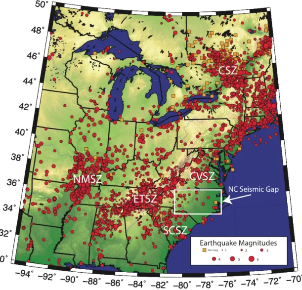
(Bollinger 1973; Figure 1). Earthquakes concentrate in known seismic zones such as the Central
Virginia Seismic Zone (Bollinger 1973), location of the 2011 MW 5.8 Mineral, VA earthquake
(Wolin et al. 2012), the South Carolina Seismic Zone (Bollinger 1973, Tarr et al. 1981, Dewey
1988), location of the 1886 MW 7.3 Charleston, SC earthquake (Tarr et al. 1981, Talwani 1982),
and the Eastern Tennessee Seismic Zone (Bollinger 1973, Powell et al. 1994, Chapman et al.
1997). Central and eastern North Carolina, where far fewer and smaller earthquakes have been
recorded, lies between these regions of elevated seismicity. Between 1973 and 2006, there were
83 earthquakes MW 2.0 or greater in Virginia and 84 in South Carolina east of the Appalachian
Mountains, but only eleven in North Carolina east of the Appalachians
(earthquake.usgs.gov/earthquakes/search/). This region of reduced seismicity, the North
Carolina seismic gap, has been recognized for some time (Sbar and Sykes 1973, Bollinger 1973),
but without correlation with major tectonic structures, it lacks an obvious tectonic explanation.
The apparent quiescence in North Carolina coincides with a lack of available passive
seismic data. There are only four seismic stations east of the Appalachians in North Carolina
with data included in the Incorporated Research Institutions for Seismology (IRIS) Data
Management Center (DMC) database prior to this study: the Penn State Network’s NCAT
station, the Appalachian Seismic Transect’s LARA station, and the United States National
Seismic Network’s CEH and CNNC stations (www.iris.edu/dms/nodes/dmc/). Thus, it is
possible that the apparent sparsity of earthquakes in central and eastern North Carolina is due to
insufficient station coverage. In order to investigate the hypothesis that the apparent quiescence
around the Deep River Basin. As discussed below, the Deep River Basin is a comparatively
recent zone of extension and may therefore be considered the most likely location for seismicity
in central and eastern North Carolina.
1.3. The Deep River Basin and hydraulic fracturing
The Deep River Basin is one of a series of Triassic rift basins along the east coast of the
United States that make up the Newark Supergroup (Olsen et al. 1989). The supergroup of
basins formed from preliminary extension during the breakup of Pangaea before the Atlantic
Ocean began to spread (Olsen et al. 1989). The Deep River Basin consists of three sub-basins,
the Wadesboro sub-basin, the Sanford sub-basin, and the Durham sub-basin (Olsen et al. 1989).
A bed of shale and coal known as the Cumnock formation surfaces along the northern margin of
the Sanford sub-basin (Olsen et al. 1991). In the past, this has been exploited by coal mining
operations. More recently, however, it has been the focus of local gas companies. Recent
legislation suggests that hydraulic fracturing operations may occur in the Sanford sub-basin in
the near future. While hydraulic fracturing itself does not cause seismicity large enough to be
recorded by the type of data analyzed here, the reinjection of wastewater into basement rocks has
been linked to more significant seismicity in certain areas. Although it is unknown whether or
not hydraulic fracturing or the associated reinjection of wastewater will occur in the Sanford
sub-basin, a baseline of natural seismicity can be recorded before operations to be used for any
2. Data and Methods
In order to study the natural seismicity of the Deep River Basin, I assisted in the
deployment of the Pre-Hydrofracking Regional Assessment of Central Carolina Seismicity
(PHRACCS) network. This deployment consists of twelve stations in a ~50 x 50 km array with
~5-15 km station spacing throughout the Sanford sub-basin of the Deep River Basin (Figure 2).
The seismometers are STS-2 broadband sensors recording at a sampling rate of 40 Hz. All of the
stations, with the exception of the northernmost (NC01), westernmost (NC02), and easternmost
(NC06) stations are located within the Deep River Basin.
Seismic events were detected using the dbdetect and dbgrassoc programs from Boulder
Real Time Technologies’ Antelope software (www.brtt.com). To detect seismic event arrivals,
we employed a Short Term Average/Long Term Average (STA/LTA) ratio method. An event
was detected when the threshold STA/LTA ratio of 3 was met by at least eight stations within a
1.5 second window, signifying the arrivals were likely of the same event. This low threshold
identified many false signals in addition to discrete earthquake-like seismic events. To remove
false signals, I filtered the detections to leave only events with an identifiable P-wave and
S-wave arrival on at least eight stations.
Event hypocenters were calculated using the Hypocenter program (Leinert et al. 1986)
included with the SEISAN seismic analysis software package (Havskov and Ottemöller 1999).
For each event-station pair, I picked all discernable P-wave and S-wave arrivals on the vertical
and transverse components, respectively. S-wave picks were ranked to represent pick
confidence. Picks were ranked as “1” when the picks were clear and impulsive arrivals. Picks
were ranked as “2” when they were clear, but not impulsive, S-wave arrivals and the precise
from Bonini and Woollard (1960) and Olsen et al. (1991) (See 2.1. Velocity Model Calibration).
Events with latitude or longitude errors greater than 5 km and events located more than 6 km
outside of the array were not included in further analysis.
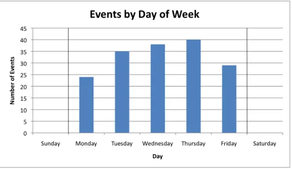
In order to evaluate possible sources for recorded events, I examined satellite images of
the event locations on Google Maps. I then compiled histograms of event source times by local
time of day and day of the week (Figures 3 and 4). As discussed in the results and discussion
sections, most of the events were located near an observable quarry and all occurred during
business hours, suggesting an anthropogenic source.
2.1. Velocity model calibration
Based on the assumption that the 136 events located near quarries are recorded quarry
blasts, I developed an optimized 1-D velocity model for locating seismic events in the Deep
River Basin. The center of each quarry is assumed to be the “true” location for events in that
cluster, providing a ground truth estimate of goodness of fit between calculated event locations
and the nearest quarry. In order to test for the optimized velocity model, I selected 29 events
with a location confirmed by the source that had the highest number of easily picked P-wave
arrivals. I then calculated the average distance between the calculated epicenter and the known
source location. In order to remove error induced by depth calculations while testing various
velocity models, I fixed hypocenter depths to 0 km. I removed S-wave picks with a ranking of 2
in order to use only the most reliable data for this calibration.
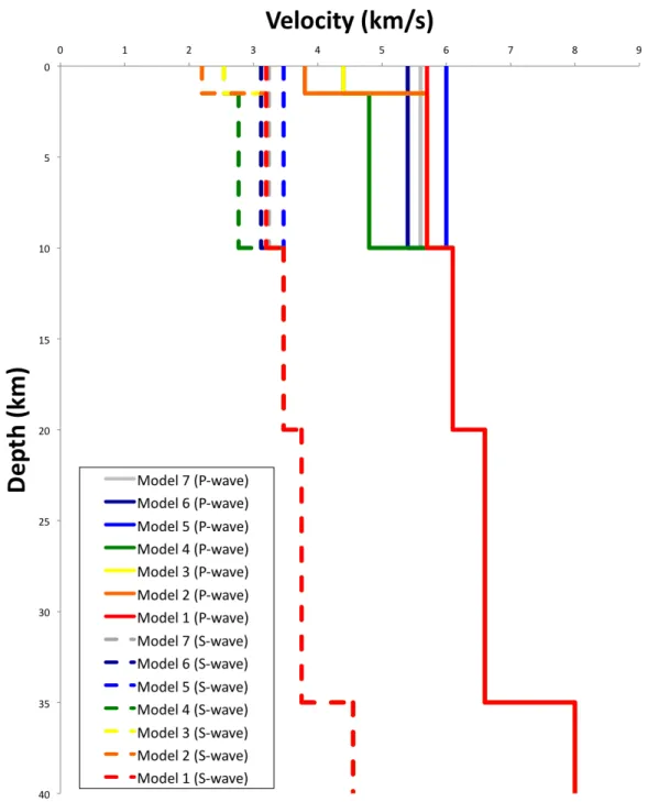
I relocated the events with each of the seven velocity models shown in Figure 5. These
include models which test the effects of adding a 1.5 km deep slow sedimentary basin layer
constraints provided by Bonini and Woollard (1960), with P-wave velocities in the basin
between 3.2-4.4 km/s and in the upper crust between 4.8-5.8 km/s. Mid- and lower-crustal
velocities are derived from seismic refraction studies in Tennessee and Missouri and off the
mid-Atlantic coast (Catchings 1999, Holbrook et al. 1992). The tested models vary velocities in the
basin and the upper crust within the constraints of Bonini and Woollard (1960) while leaving the
mid-crust through upper mantle unchanged (Figure 5). I used the best fitting velocity model
(Velocity Model 1) for the final locations presented in this study.
2.2. Event magnitude determination
I calculated local event magnitudes (ML) for each event using the MULPLT and
Hypocenter (Leinert et al. 1986) programs within SEISAN (Havskov and Ottemöller 1999). For
each event, I converted the seismograms to match the response of a Wood-Anderson
seismograph using MULPLT (Havskov and Ottemöller 1999). This automatically determines
maximum displacement amplitude on the vertical component of the Wood-Anderson
seismogram. Using Hypocenter (Leinert et al. 1986), I calculated ML for each station-event pair
with distance from the event and the maximum displacement amplitude. For each event, we
consider the average ML of all stations to be the event’s ML (Figure 6). I calculated standard
3. Results
After removing poorly constrained events from the dataset, I found 166 events that were
locatable within or close to the PHRACCS array between March 30, 2012 and July 3, 2013. The
event epicenters fall into four distinct clusters, with one exception (Figure 7). Two clusters
(Clusters 1 and 2), consisting of 97 events total, are located northeast of the array. Cluster 3,
consisting of 38 events, is located southeast of the array. Cluster 4, consisting of 30 events, is
located in the center of the array around station NC04. The last event is located on the
southwestern edge of the array.
Clusters 1, 2, and 3 are co-located with the Luck Stone Pittsboro Plant quarry, the Wake
Stone Corporation quarry, and the Martin Marietta Aggregates Lemon Springs Quarry,
respectively (Figure 8). Cluster 4 is located in Cumnock near the site of the abandoned Egypt
Coal Mine and is not associated with an obvious quarry. All recorded events occurred between
9am and 5pm local time on Monday through Friday. The spatial and temporal association of the
events with business activities suggests that the events are the result of quarry blasts and other
human activities. In order to validate this association, I contacted two of the event source
quarries by phone. The Luck Stone Pittsboro Plant confirmed they had an explosion coincident
with the origin time of each event recorded in Cluster 1 from January to June 2013. The Wake
Stone Corporation confirmed they had an explosion coincident with the origin time of each event
recorded in the cluster from April 2012 to June 2013. I was unable to reach the Martin Marietta
Aggregates Lemon Springs Quarry (Cluster 3). No source for Cluster 4 was contacted because
its source remains ambiguous, but two observations suggest that the events are likely
exception (Figures 3 and 4) and 2) the seismograms for these events are indiscernible from the
seismograms from the confirmed quarry blasts (Figure 9).
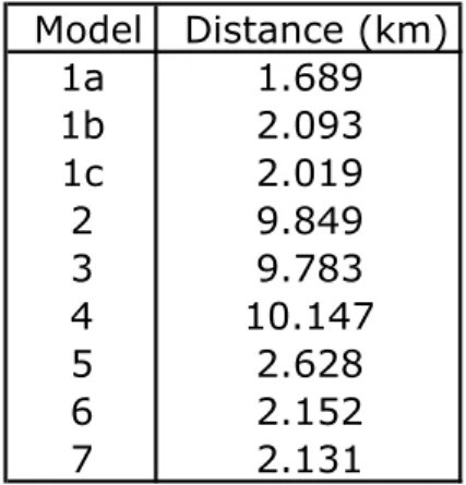
The results of the velocity model calibration indicate that velocity models with a
sedimentary basin yield significantly less accurate locations than those without a basin included
(See Velocity Models 2-4 in Table 1). Figures 10, 11, and 12 show the locations calculated for
each velocity model. Velocity Model 1 locates events most accurately, placing events on
average 2.019 km from their respective sources. However, Velocity Model 1 located events best
when depth was left free and S-wave picks ranked 2 were included in calculations, locating
events on average 1.689 km from their respective sources (See Velocity Model 1a in Table 1), so
locations in this study were calculated with these conditions.
Considering the known quarries as the source locations for Clusters 1, 2, 3, and the
outlying event, we relocated the events with Velocity Model 1. All of the events with a known
source located at their respective sources within error (Figure 13).
The calculated error for event locations using Velocity Model 1 ranges from 0.6-4.3 km
in latitude and 0.9-3.8 km in longitude. Calculated hypocenter depths range from 0.7-8.1 km
with 1.6-10.4 km error. However, 139 of 166 events were located within 2 km of their
respective source, showing that hypocenter error is more likely on the order of 2 km using the
PHRACCS array.
The results of the magnitude determinations show recorded local magnitudes of 0.7-1.7
(Figure 6). For a given station, magnitudes were calculated as low as 0.2 and as high as 2.4. An
analysis of the scatter of magnitude values for each station shows that on average, each station
deviates from the mean by no more than 0.2, showing that there is no large systematic error
than 0.1. This error is likely the result of variable attenuation reducing or enhancing amplitudes
at a given station and/or, error in epicenter locations effecting calculated distances (described
4. Discussion
4.1. Tectonic implications
The apparent lack of natural seismicity in the Deep River basin strongly suggests that the
observed along-strike variability in seismic moment release in the southeastern United States is
not due to variable sampling. A more recent catalog of earthquakes with TA’s uniform station
sampling confirms the variation in seismicity (earthquake.usgs.gov/earthquakes/search/).
Determining the cause of this variability is difficult because of the lack of seismic data
recorded in the region (See Introduction). A potential source for variation between North
Carolina and the surrounding states is the Cape Fear Arch, a prominent feature of raised
basement extending inland from the coast (Soller 1988). However, there has not been a
comprehensive correlation between the Cape Fear Arch and seismic patterns. Recent seismic
studies in the eastern United States have not had clear enough resolution surrounding North
Carolina to identify small-scale variations in structure such as the Cape Fear Arch (van der Lee
et al. 2008, Bedle and van der Lee 2009, Sigloch 2011).
The aforementioned studies on the causes of intraplate seismicity suggest that the Cape
Fear Arch or another as yet unknown variation in inherited lithospheric structure may be able to
explain the variable seismicity in the eastern United States. However, further seismic studies
across the region by Earthscope’s TA or FlexArray will be necessary to look at North Carolina’s
subsurface with higher resolution.
4.2. PHRACCS detection capabilities and implications for hydraulic fracturing
Although no natural earthquakes were recorded by the PHRACCS array, the recorded
able to consistently locate quarry blasts within 2 km of their source quarry. This allows us to
constrain the accuracy of the locations we are able to calculate using the array. Further, the array
was able to consistently record locatable quarry blasts at ML > 0.8 (Figure 6), with only four
blasts < ML 0.9 confidently recorded above background noise.
It is expected that hydraulic fracturing operations will occur in the Sanford sub-basin to
exploit a reported large repository of shale gas in the Cumnock formation. The constraints on
our ability to detect and locate events using the PHRACCS array indicate the array’s utility in the
event of local hydraulic fracturing and wastewater reinjection. The process of hydraulic
fracturing produces many earthquakes, but these earthquakes are rarely strong enough to be felt
(Ellsworth 2013). The majority of earthquakes produced by hydraulic fracturing are of moment
magnitude (MW) <0 (Davies et al. 2013, Holland 2013), which is much smaller than the events
located with the PHRACCS array. Traditionally, studies of microseismicity induced by
hydraulic fracturing require dense arrays of borehole seismometers that can locate extremely
small earthquakes within meter scale error (House 1987, Davies et al. 2013, Raleigh et al. 1976,
Rutledge et al. 2004). PHRACCS can only locate events accurately to within 2 km, which is not
precise enough to study such induced earthquakes (Davies et al. 2013).
The PHRACCS array will, however, be useful in the event of local wastewater
reinjection. There are several cases of large earthquakes being attributed to wastewater
reinjection, but there is generally not a comprehensive baseline of seismicity for comparison to
confirm that earthquakes did not previously occur naturally (Holland 2013). Such earthquakes
are frequently MW > 3 and in some cases reach greater than MW 5, such as the 2011 MW 5.7 in
Oklahoma (Keranen et al. 2013). This study provides a detailed baseline of natural seismicity in
natural seismicity recorded by PHRACCS consists of no confirmed natural earthquakes in the
Sanford sub-basin during the fifteen months analyzed for this study. The data from this study are
5. Conclusions
We investigate the North Carolina seismic gap by looking for previously unrecorded
earthquakes with a dense array of broadband seismometers in the Triassic Deep River Basin.
Due to the extensive seismicity in surrounding regions, such as the South Carolina Seismic Zone,
the Central Virginia Seismic Zone, and the Eastern Tennessee Seismic Zone, we expected to
record earthquakes in North Carolina. The results of this investigation can be summarized in
three main conclusions:
1) The North Carolina seismic gap is a robust observation and is not due to a lack of
regional seismic data.
2) The PHRACCS array confidently recorded and located seismic events down to ML 0.9
± 0.1. Events can accurately be located within 2 km of their sources.
3) We have found no evidence of natural earthquakes with ML > 0.8, in the Sanford
sub-basin of the Deep River Basin between May 28, 2012 and July 3, 2013. This may be used as a
6. References
Assumpção, M., M. Schimmel, C. Escalante, J.R. Barbosa, M. Rocha, and L.V. Barros (2004).
Intraplate seismicity in SE Brazil: stress concentration in lithospheric thin spots.
Geophysical Journal International, 159, 390-399.
Babuska, V., J. Plomerova, and T. Fischer (2007). Intraplate seismicity in the western Bohemian
Massif (central Europe): A possible correlation with a paleoplate junction. Journal of
Geodynamics, 159(1), 390-399.
Bartholomew, M.J. (1983). Palinspastic reconstruction of the Grenville terrane in the Blue Ridge
Geologic Province, southern and central Appalachians, U.S.A. Geological Journal, 18,
241-253.
Bartholomew, M.J. and R.B. Van Arsdale (2012). Structural controls on intraplate earthquakes in
the eastern United States. Recent Advances in North American Paleoseismology and
Neotectonics East of the Rockies, 493, 165-189.
Bedle, H. and S. van der Lee (2009). S velocity variations beneath North America.
Journal of Geophysical Research, 114, B07308.
Bollinger, G.A. (1973). Seismicity and crustal uplift in the southeastern United States. American
Journal of Science, Cooper 273-A, 396-408.
Bonini, W.E. and G.P. Woollard (1960). Subsurface Geology of North Carolina-South
Carolina Coastal Plain from Seismic Data. AAPG Bulletin, 44, 298-315.
Bräuer, K., H. Kämpf, G. Strauch, and S.M. Weise (2003). Isotopic evidence (3He/4He, 13CCO2)
of fluid-triggered intraplate seismicity. Journal of Geophysical Research, 108, 2070.
Catchings, R.D. (1999). Regional Vp, Vs, Vp/Vs, and Poisson’s Ratios across Earthquake
Seismological Society of America, 89, 1591-1605.
Chapman, M.C., C.A. Powell, G. Vlahovic, and M.S. Sibol (1997). A Statistical Analysis of
Earthquake Focal Mechanisms and Epicenter Locations in the Eastern Tennessee Seismic
Zone. Bulletin of the Seismological Society of America, 87(6), 1522-1536.
Chapman, M.C. and J.N. Beale (2010). On the Geologic Structure at the Epicenter of the 1886
Charleston, South Carolina, Earthquake. Bulletin of the Seismological Society of
America, 100, 1010-1030.
Costain, J.K. (2008) Intraplate Seismicity, Hydroseismicity, and Predictions in Hindsight.
Seismological Research Letters, 79, 578-589.
Davies, R., G. Foulger, A. Bindley, and P. Styles (2013). Induced seismicity and hydraulic
fracturing for the recovery of hydrocarbons. Marine and Petroleum Geology, 45, 171-185.
Dewey, J.W. (1988). Midplate seismicity exterior to former rift-basins. Seismological Research
Letters, 59(4), 213-218.
Ellsworth, W.L. (2013). Injection-induced earthquakes. Science, 341, 1225942.
Fletcher, J.B., M.L. Sbar, and L.R. Sykes (1978). Seismic trends and travel-time residuals in
eastern North America and their tectonic implications. Geological Society of America
Bulletin, 89, 1656-1676.
Hatcher, R.D. (2010). The Appalachian orogen: a brief summary. In: Tollo, R.P., M.J.
Bartholomew, J.P. Hibbard, and P.M. Karabinos (Eds.), From Rodinia to Pangea: The
Lithotectonic record of the Appalachian Region, 1-19.
Havskov, J. and L. Ottemöller (1999). SeisAn Earthquake Analysis Software. Seismological
Research Letters, 70, 532-534.
Geology, 58, 127-130.
Hibbard, J.P., E.F. Stoddard, D.T. Secor, and A.J. Dennis (2002). The Carolina Zone:
overview of Neoproterozoic to Early Paleozoic peri-Gondwanan terranes along the
Eastern Flank of the southern Appalachians. Earth-Science Reviews, 57, 299-339.
Hoffman, P.F. (1991). Did the Breakout of Laurentia Turn Gondwanaland Inside Out? Science,
252(5011), 1409-1412.
Holbrook, W.S., G.M. Purdy, J.A. Collins, R.E. Sheridan, D.L. Musser, L. Glover III, M.
Talwani, J.I. Ewing, R. Hawman, and S.B. Smithson (1992). Deep Velocity
Structure of Rifted Continental Crust, U.S. Mid-Atlantic Margin, from Wide Angle
Reflection/Refraction Data. Geophysical Research Letters, 19, 1669-1702.
Holland, A.A. (2013). Earthquakes Triggered by Hydraulic Fracturing in South Central
Oklahoma. Bulletin of the Seismological Society of America, 103, 1784-1792.
House, L. (1987). Locating Microearthquakes Induced by Hydraulic Fracturing in Crystalline
Rock. Geophysical Research Letters, 14, 919-921.
Johnston, A.C. and L.R. Kanter (1990). Earthquakes in Stable Continental Crust. Scientific
American, March, 68-75.
Keranen, K.M., H.M. Savage, G.A. Abers, and E.S. Cochran (2013). Potentially induced
earthquakes in Oklahoma, USA: Links between wastewater injection and the 2011 MW
5.7 earthquakes sequence. Geology, 41, 699-702.
Leinert, B.R., E. Berg, and L.N. Frazer (1986). Hypocenter: An Earthquake Location Method
Using Centered, Scaled, and Adaptively Damped Least Squares. Bulletin of the
Seismological Society of America, 76, 771-783.
central-eastern United States: Insights from geodynamic modeling. Geological Society of
America Special Paper, 425, 149-166.
Li, Q., M. Liu, and S. Stein (2009). Spatiotemporal Complexity of Continental Intraplate
Seismicity: Insights from Geodynamic Modeling and Implications for Seismic Hazard
Estimation. Bulletin of the Seismological Society of America, 99(1), 52-60.
Liu, L. and M.D. Zoback (1997). Lithospheric strength and intraplate seismicity in the New
Madrid seismic zone. Tectonics, 16, 585-595.
McBride, J.H. and K.D. Nelson (1988). Integration of COCORP deep reflection and magnetic
anomaly analysis in the southeastern United States: Implications for origin of the
Brunswick and East Coast magnetic anomalies. Geological Society of America Bulletin,
100, 436-445.
Miller, B.V., A.H. Fetter, and K.G. Stewart (2006). Plutonism in three orogenic pulses, Eastern
Blue Ridge Province, southern Appalachians. Geological Society of America Bulletin,
118(1/2), 171-184.
Mooney, W.D., J. Ritsema, and Y.K. Hwang (2012). Crustal seismicity and the earthquake
catalog maximum moment magnitude (Mcmax) in stable continental regions (SCRs):
Correlation with the seismic velocity of the lithosphere. Earth and Planetary Science
Letters, 357-358, 78-83.
Olsen, P. E., R. W. Schlische, and P. J. W. Gore (1989). Tectonic, Depositional, and
Paleoecological History of Early Mesozoic Rift Basins, Eastern North America, Field
Olsen, P. E., A.J. Froelich, D.L. Daniels, J.P. Smoot and P.J.W. Gore (1991). Rift basins of early
Mesozoic age, in Horton, W., ed., Geology of the Carolinas, University of Tennessee
Press, Knoxville, 142-170.
Powell, C.A., G.A. Bollinger, M.C. Chapman, M.S. Sibol, A.C. Johnston, and R.L. Wheeler
(1994). A Seismotectonic Model for the 300-Kilometer-Long Eastern Tennessee Seismic
Zone. Science, 264(5159), 686-688.
Raleigh, C.B., J.H. Healy, and J.D. Bredehoeft (1976). An Experiment in Earthquake Control at
Rangely, Colorado. Science, 191, 1230-1237.
Rankin, D.W. (1976). Appalachian Salients and Recesses: Late Precambrian Continental
Breakup and the Opening of the Iapetus Ocean. Journal of Geophysical Research, 81(32),
5605-5619.
Rivers, T. (1997). Lithotectonic elements of the Grenville Province: review and tectonic
implications. Precambrian Research, 86, 117-154.
Rutledge, J.T., W.S. Phillips, and M.J. Mayerhofer (2004). Faulting Induced by Forced Fluid
Injection and Fluid Flow Forced by Faulting: An Interpretation of Hydraulic-Fracture
Microseismicity, Carthage Cotton Valley Gas Field, Texas. Bulletin of the Seismological
Society of America, 94, 1817-1830.
Sbar, M.L. and L.R. Sykes (1973). Contemporary Compressive Stress and Seismicity in Eastern
North America: An Example of Intra-Plate Tectonics. Geological Society of America
Bulletin, 84, 1861-1882.
Sigloch, K. (2011). Mantle provinces under North America from multifrequency P-wave
Soller, D.R. (1988). Geology and tectonic history of the lower Cape Fear river valley,
southeastern North Carolina. United States Geological Survey Professional Paper, 1466.
Swafford, L. and S. Stein (2007). Limitations of the short earthquake record for seismicity and
seismic hazard studies. Geological Society of America Special Paper,425, 49-58.
Sykes, L.R. (1978). Intraplate Seismicity, Reactivation of Preexisting Zones of Weakness,
Alkaline Magmatism, and Other Tectonism Postdating Continental Fragmentation.
Reviews of Geophysics and Space Physics, 16, 621-688.
Talwani, P. (1982). Internally consistent pattern of seismicity near Charleston, South Carolina.
Geology, 10, 654-658.
Talwani, P. (1988). The intersection model for intraplate earthquakes. Seismological Research
Letters, 59(4), 305-310.
Tarr, A.C., P. Talwani, S. Rhea, D. Carver, and D. Amick (1981). Results of Recent South
Carolina Seismological Studies. Bulletin of Seismological Society of America, 71,
1883-1902.
Thomas, W.A. (2006). Tectonic inheritance at a continental margin. Geological Society of
America Today, 16(2), 4-11.
van der Lee, S., K. Regenauer-Lieb, and D.A. Yuen (2008). The role of water in connecting past
and future episodes of subduction. Earth and Planetary Science Letters, 273, 15-27.
Williams, H. and R.N. Hiscott (1987). Definition of the Iapetus rift-drift transition in western
Newfoundland. Geology, 15, 1044-1047.
Wolin, E., S. Stein, F.Pazzaglia, A. Meltzer, A. Kafka, and C. Berti (2012). Mineral, Virginia,
earthquake illustrates seismicity of a passive-aggressive margin. Geophysical Research
Zoback, M.L. (1992). Stress Field Constraints on Intraplate Seismicity in Eastern North
7. Tables
Table 1: The results of velocity model testing. Models 1-7 can be seen in Figure 5. Model 1a is
Velocity Model 1 with all S-wave arrival picks and a free depth. Model 1b is Velocity Model 1
with Ranking 2 wave arrival picks removed and 1c is Velocity Model 1 with Ranking 2
S-wave arrival picks removed and depth fixed at 0 km. Distances are average distances to the
events’ respective source.
Model Distance (km)
1a 1.689
1b 2.093
1c 2.019
2 9.849
3 9.783
4 10.147
5 2.628
6 2.152
8. Figures
Figure 1: Map of seismicity in the eastern United States and Canada between 1568-2006
(www.geol.vt.edu/outreach/vtso/anonftp/catalog). The North Carolina seismic gap (NC Seismic
Gap), South Carolina Seismic Zone (SCSZ), Eastern Tennessee Seismic Zone (ETSZ), Central
Virginia Seismic Zone (CVSZ), New Madrid Seismic Zone (NMSZ) and Charlevoix Seismic
Figure 2: PHRACCS station map in relation to the Deep River Basin in North Carolina.
Figure 5: Velocity models tested. Solid lines are P-wave velocities for each model. Dashed
lines are S-wave velocities for each model. The red lines represent the model used for locations
Figure 7: Map of recorded seismic events in relation to associated anthropogenic source and
PHRACCS stations. The four clusters of events are labeled. Boxes show the locations of the
Figure 8: Satellite images from Google Maps showing each cluster of events. Each image
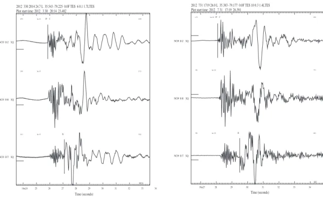
Figure 9: Sample seismograms of vertical, radial, and transverse components for a single station
for two events. On the left are the seismograms recorded at station NC03 for an event in Cluster
4. On the right are the seismograms recorded at station NC09 for an event in Cluster 3. The
event on the left does not have a confirmed source whereas the event on the right is confirmed as
a quarry blast.
!"#!$$%%"$!"#&$!&'($)$$%*'*&%$+(,'!!*$$"'"-$./0$$1$"'#$#'()./0$$$$$$$$$$$$$$$$ 2345$65785$59:;<$!"#!$$$%$%"$$$!"<#&$$!%'&=!$$$$$$$$$$$$$$$$$$$$ $$$$$$$##"*% $$$$$$$$!=(, >7?$$=* @A"%$$B$C$$$$DE F2$$$$$A$$ $$$$$$$##(## $$$$$$$$!%", >7?$$=* @A"%$$B$G$$$$DE 0/A
#&:!& !* !1 !( != !, %" %# %! %% %&
$$$$$$$#!#"# $$$$$$$$#=!% >7?$$=* @A"%$$B$.$$$$DE F0$$$$$$$$ !"#!$$(%#$#(#,$!1'"$)$$%*'%=%$+(,'#(($$"'"-$./0$#"$"'%$#'&)./0$$$$$$$$$$$$$$$$ 2345$65785$59:;<$!"#!$$$($%#$$$#(<#,$$!1'%,#$$$$$$$$$$$$$$$$$$$$ $$$$$$$$1(", $$$$$$$+##(* >7?$#!= @A",$$B$C$$$$DE F2$$$$$A$$ $$$$$$$$(%(# $$$$$$$$+,!1 >7?$#!= @A",$$B$G$$$$DE 0/A
#,:!( != !, %" %# %! %% %&
$$$$$$$$1&"#
$$$$$$$$$,,= >7?$#!=
@A",$$B$.$$$$DE
F0$$$$$$$$
Figure 10: Maps showing event locations using each tested velocity model. On the left is the
map and on the right is the corresponding velocity model, showing P-wave velocity with a solid
line and S-wave velocity with a dashed line. Top is Velocity Model 1A, middle is Velocity
Model 1B, and bottom is Velocity Model 1C.
ïÝ ïÝ ïÝ
Ý Ý
Ý Ý
! "#
ïÝ ïÝ ïÝ
Ý Ý
Ý Ý
ïÝ ïÝ ïÝ
Ý Ý
Ý Ý
ïÝ ïÝ ïÝ
Ý Ý
Ý Ý
ïÝ ïÝ ïÝ
Ý Ý
Ý Ý
! "#
ïÝ ïÝ ïÝ
Ý Ý
Ý Ý
ïÝ ïÝ ïÝ
Ý Ý
Ý Ý
ïÝ ïÝ ïÝ
Ý Ý Ý Ý ïÝ ïÝ ïÝ ïÝ ïÝ ïÝ Ý Ý Ý Ý
! "#
Figure 11: Maps showing event locations using each tested velocity model. On the left is the
map and on the right is the corresponding velocity model, showing P-wave velocity with a solid
line and S-wave velocity with a dashed line. Top is Velocity Model 2, middle is Velocity Model
3, and bottom is Velocity Model 4.
ïÝ ïÝ ïÝ
Ý Ý
Ý Ý
! "#
ïÝ ïÝ ïÝ
Ý Ý
Ý Ý
ïÝ ïÝ ïÝ
Ý Ý
Ý Ý
ïÝ ïÝ ïÝ
Ý Ý Ý Ý ïÝ ïÝ ïÝ ïÝ ïÝ ïÝ Ý Ý Ý Ý
! "#
ïÝ ïÝ ïÝ ïÝ ïÝ ïÝ Ý Ý Ý Ý ïÝ ïÝ ïÝ ïÝ ïÝ ïÝ Ý Ý Ý Ý ïÝ ïÝ ïÝ ïÝ ïÝ ïÝ Ý Ý Ý Ý
ïÝ ïÝ ïÝ
Ý Ý
Ý Ý
! "#
ïÝ ïÝ ïÝ
Ý Ý
Ý Ý
ïÝ ïÝ ïÝ
Ý Ý
Ý Ý
ïÝ ïÝ ïÝ
Ý Ý
Figure 12: Maps showing event locations using each tested velocity model. On the left is the
map and on the right is the corresponding velocity model, showing P-wave velocity with a solid
line and S-wave velocity with a dashed line. Top is Velocity Model 5, middle is Velocity Model
6, and bottom is Velocity Model 7.
ïÝ ïÝ ïÝ ïÝ ïÝ ïÝ Ý Ý Ý Ý
! "#
ïÝ ïÝ ïÝ ïÝ ïÝ ïÝ Ý Ý Ý Ý ïÝ ïÝ ïÝ ïÝ ïÝ ïÝ Ý Ý Ý Ý ïÝ ïÝ ïÝ ïÝ ïÝ ïÝ Ý Ý Ý Ý
ïÝ ïÝ ïÝ
Ý Ý
Ý Ý
! "#
ïÝ ïÝ ïÝ
Ý Ý
Ý Ý
ïÝ ïÝ ïÝ
Ý Ý
Ý Ý
ïÝ ïÝ ïÝ
Ý Ý
Ý Ý
ïÝ ïÝ ïÝ
Ý Ý
Ý Ý
! "#
ïÝ ïÝ ïÝ
Ý Ý
Ý Ý
ïÝ ïÝ ïÝ
Ý Ý
Ý Ý
ïÝ ïÝ ïÝ
Ý Ý
Figure 13: Plot of calculated epicenter error (km) versus distance to event source (km). The
blue line is a simple line of y = x. Events plotted above the line were located accurately within