LEARNING ADAPTIVE REPRESENTATIONS FOR IMAGE RETRIEVAL AND RECOGNITION
Hyo Jin Kim
A thesis submitted to the faculty at the University of North Carolina at Chapel Hill in partial fulfillment of the requirements for the degree of Doctor of Philosophy in the
Department of Computer Science.
Chapel Hill 2018
©2018 Hyo Jin Kim
ABSTRACT
Hyo Jin Kim: Learning Adaptive Representations for Image Retrieval and Recognition (Under the direction of Jan-Michael Frahm)
Content-based image retrieval is a core problem in computer vision. It has a wide range of application such as object and place recognition, digital library search, organizing image collections, and 3D reconstruction. However, robust and accurate image retrieval from a large-scale image collection still remains an open problem. For particular instance retrieval, challenges come not only from photometric and geometric changes between the query and the database images, but also from severe visual overlap with irrelevant images. On the other hand, large intra-class variation and inter-class similarity between semantic categories represents a major obstacle in semantic image retrieval and recognition.
ACKNOWLEDGEMENTS
I would like to thank Jesus for his grace, guidance, protection, and provisions throughout my life, including my journey to PhD, from the application to the defense, and beyond.
I am blessed to be advised by Prof. Jan-Michael Frahm, who took me under his wing and helped me to develop as a researcher and a person. Without his help and guidance, this work would not have been possible. I deeply appreciate his encouragement and extensive support throughout the years. Especially, I am grateful for his patience and providing me the freedom to explore and develop ideas on my own. I would further like to thank his lovely family for kindly inviting us over for celebrations, and for the fun memories.
I would also like to extend my gratitude to my wonderful committee for their genuine investment on my work as well as their kind support. I had a great pleasure working with Prof. Enrique Dunn, who provided valuable input on this work. His trust and support also meant a lot to me. My sincere thanks goes out to Prof. Alex Berg for fruitful discussions, crucial research advice when I was facing obstacles, and always willing to help me. Many thanks to Prof. Marc Niethammer for being a great teacher, for giving me the opportunity to help teach his class, as well as for his help and encouragement during my tough times. I am deeply grateful to Dr. Torsten Sattler, on whose work I have drawn upon since the beginning of my PhD study, for his insightful and sharp feedback on this work.
In addition, I must thank the researchers who generously provided me with the data and code, as well as the answers to my questions: Dr. Amir Zamir, Dr. Relja Arandjelovi´c, Prof. Akihiko Torii, Dr. Giorgos Tolias, and Dr. Bolei Zhou.
Cho, Hongsheng Yang, Johannes Sch¨onberger, Rohit Gupta, True Price, Akash Bapat, Marc Eder, Zhen Wei, John Lim, Joe Tighe, Xufeng Han, Vincente Ordonez, Hadi Kiapour, Wei Liu, Sirion Vittayakorn, Eunbyung Park, Yipin Zhou, Licheng Yu, Chengyang Fu, Philip Ammirato, Patrick Poirson, Misha Shvets, Adam Aji. I would like to especially thank Jared for his help during my first two years.
Furthermore, I would like to thank Prof. Kyoung Mu Lee and Prof. Minsu Cho for their continuous support and encouragement. I am also thankful to Prof. Vladimir Jojic and Prof. Tamara Berg for their help and advice.
TABLE OF CONTENTS
LIST OF TABLES . . . x
LIST OF FIGURES . . . xii
CHAPTER 1: INTRODUCTION . . . 1
1.1 Thesis Statement . . . 5
1.2 Contributions . . . 5
1.3 Thesis Outline . . . 6
CHAPTER 2: BACKGROUND AND RELATED WORKS . . . 9
2.1 Content-Based Image Retrieval. . . 9
2.1.1 Particular Instance Retrieval . . . 9
2.1.2 Semantic Image Retrieval . . . 12
2.2 Visual Place Recognition . . . 12
2.2.1 Dealing with Geographically Ubiquitous Visual Elements . . . 14
2.2.2 Dealing with Transient Elements . . . 15
2.2.3 Use of Context Information . . . 15
2.2.4 Data-Driven Notion of Useful Visual Elements for Place Recognition . . 16
2.3 Automatic Training Data Generation . . . 17
2.4 Tree Structured Deep Neural Networks . . . 17
2.5 Scene Category Recognition . . . 19
CHAPTER 3: PREDICTING GOOD FEATURES FOR IMAGE GEO-LOCALIZATION 20 3.1 Proposed approach . . . 22
3.1.2 Predicting good features for geo-localization . . . 26
3.1.2.1 Automatic training data generation . . . 26
3.1.2.2 Closed-loop training of SVM classifiers . . . 28
3.2 Experiments . . . 30
3.2.1 Image Geo-localization . . . 30
3.2.1.1 Failure cases . . . 35
3.2.2 PBVLAD for general image retrieval . . . 36
3.3 Conclusion . . . 37
CHAPTER 4: LEARNED CONTEXTUAL FEATURE REWEIGHTING FOR IMAGE GEO-LOCALIZATION . . . 39
4.1 Method . . . 42
4.1.1 The Contextual Reweighting Network . . . 42
4.1.2 Training . . . 46
4.1.3 Image Geo-Localization . . . 49
4.1.4 Comparison of the Emphasized Features . . . 54
4.1.5 Unsupervised Discovery of Contexts for Image Geo-Localization . . . 54
4.1.6 Image Retrieval . . . 59
4.2 Contextual Feature Reweighting . . . 59
4.3 Retrieval Result: Geo-Localization . . . 60
4.4 Conclusions . . . 62
CHAPTER 5: HIERARCHY OF ALTERNATING SPECIALISTS FOR SCENE RECOGNITION . . . 65
5.1 Method . . . 68
5.1.1 Hierarchy of Alternating Specialists . . . 68
5.1.2 Discovering the areas of confusion . . . 71
5.1.3 Training . . . 73
5.2 Experiments . . . 74
5.2.1 Datasets and evaluation methodology . . . 75
5.2.2 Scene classification results . . . 76
5.2.3 Comparison with other tree-structured models . . . 79
5.2.4 Visualization of Learned Hierarchy of Specialties . . . 80
5.2.5 Comparison of Regions of Interest (ROI) . . . 81
5.2.6 Ablation Study . . . 82
5.2.6.1 Benefits of having a deeper hierarchy . . . 82
5.2.6.2 Comparison of confusing-cluster-based and coarse-category-based specialists in flat models . . . 82
5.2.7 Visualization of the mini-batch soft k-means on MNIST . . . 83
5.2.8 Computational Time . . . 84
5.3 Conclusion . . . 85
CHAPTER 6: CONCLUSION . . . 89
CHAPTER 7: FUTURE WORK . . . 91
7.1 Learned Hierarchy of Specialist for Visual Feedback in Interactive Search . . . 91
7.2 Extension to Scene-Category-Aware Place Recognition . . . 92
7.3 Extension of Hierarchy of Specialist to World-Scale Place Recognition . . . 93
7.4 Semantic Retrieval of Complicated Scenes . . . 93
7.5 Other Directions . . . 94
APPENDIX A:FAST NEAREST NEIGHBOR SEARCH . . . 95
A.0.1 Indexing using Vocabulary Tree . . . 95
A.0.2 KD-Tree . . . 96
A.0.3 Locality Sensitive Hashing (LSH) . . . 96
A.0.4 PQ Quantization . . . 97
LIST OF TABLES
Table 3.1 – Proportion of correctly localized images at top 1 . . . 32 Table 3.2 – Comparative image retrieval performance of PBVLAD on the
Ox-ford 5k dataset. The accuracy is measured by the mean Average
Precision (mAP). All descriptors are uncompressed. . . 37 Table 3.3 – Retrieval performance of PBVLAD on Oxford 5k dataset, before
and after the dimensionality reduction using PCA. The accuracy is
measured by the mean Average Precision (mAP). . . 37
Table 4.1 – Proportion of correctly localized images at top 1 . . . 51 Table 4.2 – Comparison of our proposed CRN and CroW (Kalantidis et al.,
2016) with (V)GG16 and (A)lexnet base architectures. . . 53 Table 4.3 – Comparison of using different image resolutions. All models are
based on AlexNet architecture. . . 53 Table 4.4 – Recalls on Tokyo 24/7 (Torii et al., 2015a) and Pittsburgh 250k
test (Arandjelovi´c et al., 2016) datasets. All models are based on VGG16 architecture. For NetVLAD, we used the recalls reported by authors of (Arandjelovi´c et al., 2016). We used the full resolution
images for evaluation as in (Arandjelovi´c et al., 2016). . . 54 Table 4.5 –Retrieval performance of our model trained on San Francisco on image
retrieval benchmarks Oxford 5K and 105K (Philbin et al., 2007). No cropping of ROI in the query, spatial re-ranking, or query expansion was performed. The accuracy is measured by the mean Average Precision
(mAP). All compared models are based on VGG16 architecture. . . 59
Table 5.1 – Scene classification accuracy. All compared models are based on AlexNet* (Krizhevsky, 2014) architecture. Statistics are collected
under single-view testing. . . 77 Table 5.2 – Scene classification performance of the AlexNet* (Krizhevsky, 2014)
with different global pooling schemes on SUN190 dataset. . . 78 Table 5.3 – Statistics of the AlexNet* (Krizhevsky, 2014) with global
ordered/order-less pooling on SUN190. The IoU of the correct predictions suggests
Table 5.4 – Comparison with other tree-structured models on CIFAR-100 dataset. All compared models are based on NIN-C100 (Lin et al., 2013)
ar-chitecture. Statistics are collected under single-view testing. . . 78 Table 5.5 – Comparison of hierarchical vs. flat structure (HAS vs. HAS-flat,
Fig. 5.7 (a,b)). #specialist denote the total number of specialists in the model. We report scene classification accuracy on SUN-190 dataset, using AlexNet* (Krizhevsky, 2014) architecture as a base
model. . . 83 Table 5.6 – Comparison of confusing-cluster-based specialists, HS-flat
(non-alternating) and HAS-flat ((non-alternating), and the coarse-category-based specialists ((Lin et al., 2013; Yan et al., 2015; Ahmed et al., 2016)). All these models have a flat two-level structure with a single level of specialists, using NIN-C100 (Lin et al., 2013) architecture as a base model. The performance of our proposed HAS is also shown. We report image classification accuracy on CIFAR-100 (Krizhevsky
LIST OF FIGURES
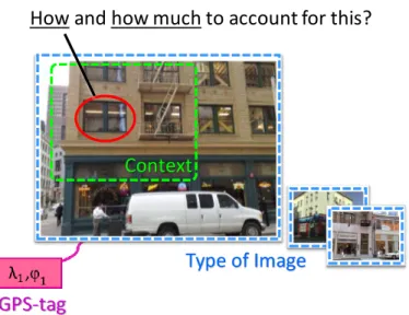
Figure 1.1 – How and how much should we account for a visual element when developing an image representation? It may depend on the type of local visual element (local context), its surroundings (semi-global
context), and the type of the image itself (global context). . . 3
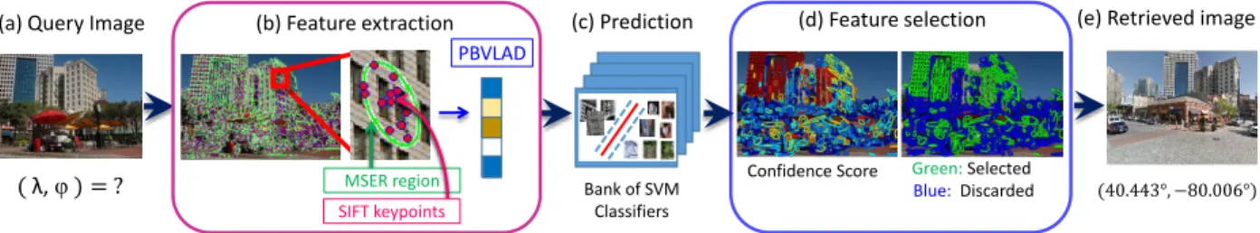
Figure 3.1 –Overview of our approach. Given an input query image with unknown geo-location (a), MSER regions and SIFT keypoint form bundled features (Wu et al., 2009), which are then represented by PBVLADs (b). Features go through a pre-trained bank of SVMs that outputs binary predictions about a feature being “good” for geo-localization (c). Predictions are accumulated to compute confidence scores for each feature (d, left). Features with high scores are selected for geo-localization (d, right). A retrieved geo-tagged image is shown in (e).
. . . 22 Figure 3.2 – PBVLAD representations of corresponding bundled features. (a,e)
Two different images depicting the same place. (b,d) Multiple SIFT features are bundled within MSER regions. (c) Each bundle is represented with VLAD. We follow the visualization scheme of (J´egou et al., 2012) where subvectors are represented in a 4x4 spatial grid with red representing negative values. Note that only non-sparse blocks that correspond to overlapping visual words of
two bundles are visualized due to space limits. . . 23 Figure 3.3 – Matching with PBVLAD with similarity threshold 0.5. . . 25 Figure 3.4 – Initial training data generation. Positive and negative training
examples are depicted in green and blue, respectively. . . 26 Figure 3.5 – Overview of our training framework. For all training images that
have GPS-tags (a), we retrieve top n images from the reference set (b-c). Positive labels are assigned to features that have higher matching score in the ground-truth reference image than in the falsely retrieved reference images, with a margin greater than thres. Negative labels are assigned in a similar manner (d). To handle noise and high intra-class variation, we use a bottom-up clustering technique, refining the positive set as well as training
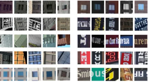
SVMs iteratively (e-f). . . 27 Figure 3.6 – Top elements in the final clusters with a high ratio of positive
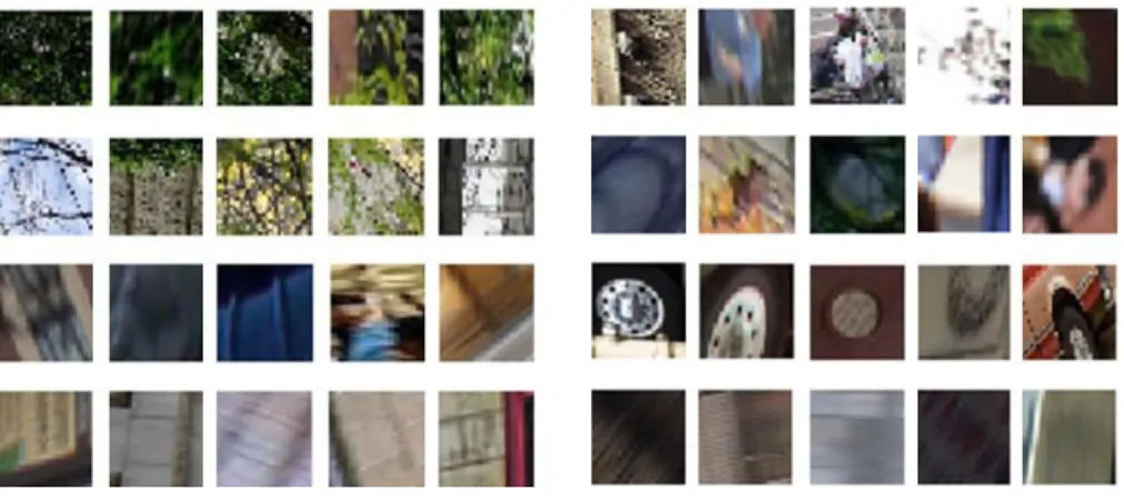
Figure 3.7 – Final negative set elements aligned according to their initial
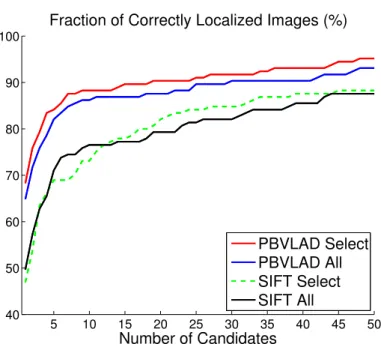
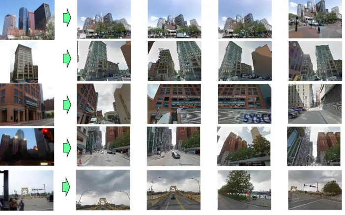
clus-ters. Each half row corresponds to different clusclus-ters. . . 30 Figure 3.8 – Geo-localization performance . . . 32 Figure 3.9 –Example result (left) Query images, (right) Top four retrieved images
using our proposed PBVLAD with feature selection. Query images are
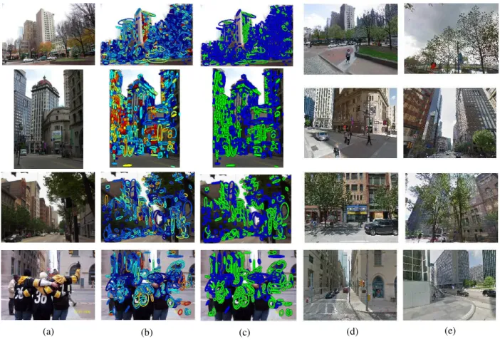
of various sizes. . . 33 Figure 3.10 –Qualitative comparison of retrieved image using selected PBVLAD and
using all of the features. (a) Query image. (b) Heat map representa-tion of the confidence of being a good feature. (c) Selected features
(green:selected, blue:discarded). (c) The top retrieved image using
selected features. (d) The top retrieved image using all features.. . . 34 Figure 3.11 –(a) Query image. (b) Heat map of maximum matching scores
maxIr(f(pq, Ir)) of all features pq. (c) Confidence scores. . . 35 Figure 3.12 –Failure cases. Retrieved images are more than 100m away from
the ground-truth locations. . . 36 Figure 3.13 –Image retrieval result on Oxford Buildings 5k dataset. (left) Query
images and average precisions (AP) by our system. (right) Top twenty retrieved images using PBVLAD as an image descriptor, where the image with the highest similarity score is shown on the top left. The green boxes around retrieved images denote the
correct retrieval results. . . 38
Figure 4.1 – Image representation with contextual feature reweighting. (a) A contextual reweighting network takes convolutional features of a deep CNN as input to produce a spatial weighting mask (b) based on the learned contexts. The mask is used for weighted aggregation of input features to produce the representation of the
input image (c). . . 40 Figure 4.2 – Contextual Reweighting Network. For each 1×1×D
convolu-tional feature, multi-scale contextual information is captured by P context filters with different window sizes (np×np×D). The filter output is then accumulated with learned weights to produce
Figure 4.3 – Overall network architecture. A CRN is a shallow network that takes the feature maps of convolutional layers as input and outputs a weighted mask indicating the importance of spatial regions in the feature maps. The resulting mask is used for performing context modulation for feature aggregation to create a global
representation of the input image. . . 44 Figure 4.4 – Recalls with and without contextual feature reweighting. . . 52 Figure 4.5 – Comparison of recalls with the state-of-the-arts methods. . . 52 Figure 4.6 – Example retrieval results on San Francisco benchmark dataset.
From left to right: query image, our contextual reweighting mask in heat map, the top retrieved image using our method, the top retrieved image using NetVLAD (Arandjelovi´c et al., 2016). Green and red borders indicate correct and incorrect retrieved results,
respectively. Results are based on our AlexNet-based model. . . 55 Figure 4.7 – Example retrieval results on San Francisco benchmark dataset.
From left to right: query image, our contextual reweighting mask in heat map, the top retrieved image using our method, the top retrieved image using NetVLAD (Arandjelovi´c et al., 2016). Green and red borders indicate correct and incorrect retrieved results,
respectively. Results are based on our AlexNet-based model. . . 56 Figure 4.8 – Comparison of emphasis on features. (first rows of heat maps below
images) Our contextual reweighting mask. (second rows of heat maps below images) NetVLAD (Arandjelovi´c et al., 2016) emphasis
on features. Both models are based on AlexNet architecture. . . 57 Figure 4.9 – Discovered data-driven contexts for image geo-localization. For
each learned context filters gp, we display image patches with top responses (Sec. 4.1.5). (Left) Filters assigned positive weights wp >0. (Right) Filters assigned negative weightswp <0. Results
are based on our AlexNet-based model. . . 58 Figure 4.10 –High weights are assigned on features from the signage on a store
front. As we removed the letters on the signage, the weights diminish. (top) Input image. (bottom) Generated contextual
Figure 4.11 –We generated synthetic images by pasting image patches containing the letters of the signage from Figure 4.10 that was assigned high weights at the store front (a-h). For (i)-(j), we overlayed the store signages from the same image on vehicles. Generated contextual reweighting masks are visualized on the bottom of each image as a heat map (red: high, blue: low). The letters from the signagage are no longer assigned high weights as the surrounding contexts
have changed. . . 61 Figure 4.12 –Image geo-localization results. (left) Query images and the
cor-responding contextual reweighting masks generated by our CRN as heat maps, (right) Top five retrieved images using our method and NetVLAD (Arandjelovi´c and Zisserman, 2014a). The green boxes around the retrieved images denote the correct results. The
results are based on our AlexNet-based model. . . 63 Figure 4.13 –Image geo-localization results. (left) Query images and the
cor-responding contextual reweighting masks generated by our CRN as heat maps, (right) Top five retrieved images using our method and NetVLAD (Arandjelovi´c and Zisserman, 2014a). The green boxes around the retrieved images denote the correct results. The
results are based on our VGG16-based model. . . 64
Figure 5.1 – (left) Similar layouts make these scenes confusing, but different objects within the scene can help determining the correct scene class. (right) While these scenes are similar in terms of content,
the layout of the scene can help distinguish between them. . . 67 Figure 5.2 – Examples of intra-class variation and inter-class similarity. While
base cabinets and bars characterize the kitchen class, it causes
overlap with other classes at the same time. . . 68 Figure 5.3 – There are subsets of images in each class that are often confused
with those of other classes. We discover confusing clusters in the feature space to disentangle intra-class variation and inter-class
similarity. . . 68 Figure 5.4 – Our proposed hierarchy of alternating specialists, where a child
model focuses on the task that is more specific than its parent. The assignment to a specialist is determined by our novel routing function, depicted as switches. The white and the blue shaded box
Figure 5.5 –(left) Input images and ground-truth category. The top-5 predictions and the visualization of class activation maps (CAM) of the top pre-dicted class for the generalist (center) and the selected specialist (right)
. . . 80 Figure 5.6 – Visualization of the learned hierarchy on the SUN190 dataset. A
three level hierarchy is shown, with the 10 top images associated
with each specialist. . . 86 Figure 5.7 –(a) Our proposed Hierarchy of Alternating Specialists. (b) Model 1,
using global-ordered pooling architecture only. (c) Model 2, using global-orderless pooling architecture only. The white and the blue
shaded box denote network architectures with different global pooling strategy. 87 Figure 5.8 –(a) Our proposed Hierarchy of Alternating Specialists (HAS). (b)
HAS-flat, a flat version of our model with single level of specialists. (c) HS-flat, a flat version of our model without thealternatingarchitecture. The white and the blue shaded box denote network architectures with
different global pooling strategy.. . . 87 Figure 5.9 – Mini-batch soft k-means result on MNIST (LeCun, 1998) dataset.
Each centroids are depicted as ⊗. (a) Pre-trained CNN with frozen parameters (only centroids µare updated) with normalized features. (b) Joint optimization of classification and clustering loss (updating both CNN parameters θ and centroids µ) with
normalized features, and with (c) unnormalized features. . . 88
CHAPTER 1: INTRODUCTION
We are living in an era where billions of digital photos, and half a billion hours of video are uploaded on the web daily (Cakebread, 2017; Nicas, 2017). Finding an image that we are interested in among those massive image collections is a challenging task. Typically, we are only interested in a few of them, while the vast majority are unrelated ones. Most of the current search engines rely on keywords and textual meta-data for searching and organizing images. However, the meta-data is often noisy and lacks description about the content of the image. Obtaining a detailed and accurate text annotation for an image, on the other hand, is expensive and impossible at times.
The objective of this thesis is to create fully-automatic systems for performing large-scale image search and recognition purely based on visual information, using only the content of an image. As the old saying goes: a picture is worth a thousand words—the amount of information that an image can contain is enormous, and it eliminates the need for manual annotations or meta-data. It can also account for visual concepts that are not easily describable by words. The applications of content-based image retrieval includes organizing photo collections (Johnson et al., 2010; Raguram et al., 2011), digital library search (Chen et al., 2011b), photo-based product search (Kiapour et al., 2015; Liu et al., 2016), reconstructing 3d models from images depicting the same place (Frahm et al., 2010; Heinly et al., 2015), and place recognition (Arandjelovi´c et al., 2016; Sattler et al., 2017).
vector, or a set of vectors. By measuring the distance between these vectors, we can compute the visual similarity between the corresponding images. The second part is to make the search efficient in terms of memory and speed. It often involves approximate nearest neighbor search, that includes quantization and indexing. This dissertation mostly focuses on the former, measuring the image similarity, which determines the accuracy of the search. A brief overview of approximate nearest neighbor search can be found in Appendix A.
How and how much to account for this?
GPS-tag
Context
Type of Image
Figure 1.1: How and how much should we account for a visual element when developing an image representation? It may depend on the type of local visual element (local context), its surroundings (semi-global context), and the type of the image itself (global context).
images of different classes. The overlap becomes more severe as the number of semantic classes increases.
In both cases, it is observed that not all of the image content is useful for a given task. Hence, instead of using all image content to represent an image, we would like our visual representations to intelligently emphasize useful regions to promote similarity to the relevant images while suppressing the regions that cause overlap to the irrelevant images. However, based on what can we discriminate these two types of image content? In this thesis, we explore three kinds of image contexts for discriminating a relevant and irrelevant image content: (1) local image context, (2) semi-global image context, and (3) global image context.
Secondly, we consider a semi-global image context. For example, again in the case of landmark retrieval, windows on buildings are useful, whereas windows on vehicle may introduce obfuscating cues (Fig. 1.1). Therefore, we design our visual representation to adaptively account for a visual element based on its semi-global context. Apart from previous work that uses supervised priors (Mousavian and Koˇsecka, 2015; Torii et al., 2015b), we take advantage of end-to-end learning such that task-relevant context emerges automatically from the data.
Thirdly, we explore the global context of the image. There are certain types of images that are easily confused. For example, the image shown in Fig. 1.1 is less likely to be confused with mountains or beach, than with the images of buildings. Thus, we take global context into account to determine which image group it belongs to. We then develop representations that are specialized for distinguishing images belonging to each particular group. Unlike previous work that organizes classes into coarse categories (Goo et al., 2016; Zhao et al., 2011; Hwang and Sigal, 2014; Deng et al., 2014), we design these groups to disentangle intra-class variation and inter-class similarity at the sub-category level.
We are not the first to consider discriminating relevant and irrelevant image content for image retrieval and recognition. However, most of the existing work relies on supervised priors for determining useful image content. The key difference that set us aside apart from the most of previous work is that we take a data-driven approach. We design our pipelines such that by training our model, the underlying task-relevant contexts are automatically discovered from the data. These include data-driven notion of good local mid-level features, task-relevant semi-global context, and hierarchy of images. Furthermore, we use minimal supervision such as gps-tags. Such a data-driven approach not only allows us to achieve better performance by analyzing the vast amount of data, which is beyond the capability of a human, but also enables our method to generalize to other tasks.
semi-global image context, and global image context. Experimental evaluation demonstrates that the resulting image representation effectively focuses on useful details to promote similarity between relevant images and to deal with visual overlap with irrelevant images in the applications of place recognition, scene categorization, particular object retrieval and object retrieval.
1.1 Thesis Statement
The robustness of image retrieval and recognition can be improved by learning image representations that adaptively focus on specific image content based on (1) local context, (2) semi-global context, and (3) global context.
1.2 Contributions
This dissertation contains several significant contributions that advanced the state of the art in image retrieval and recognition. These contributions include:
Data-driven feature selection and a novel feature description: We propose to dis-cover features that are useful for recognizing a place in a data-driven manner, and use this knowledge to predict useful features in a query image prior to the geo-localization process. This allows achieving better performance while reducing the number of features. Also, for both learning to predict features and retrieving geo-tagged images from the database, we propose a per-bundle vector of locally aggregated descriptors (PBVLAD), where each maximally stable region is described by a vector of locally aggregated descriptors (VLAD) on multiple scale-invariant features detected within the region. Experimental results show the proposed approach achieves a significant improvement over the baselines.
on regions that positively contribute to geo-localization. In particular, we introduce a Contextual Reweighting Network (CRN) that predicts the importance of each region in the feature map based on the image context. This model is learned end-to-end for the image geo-localization task, and requires no annotation other than image geo-tags for training. In experimental results, the proposed approach significantly outperforms the previous state-of-the-art on the standard geo-localization benchmark datasets. We also demonstrate that our CRN discovers task-relevant contexts without any additional supervision.
Disentangling intra-class and inter-class variation in scene categories: We propose a hierarchical generalist-specialist model that automatically builds itself based on the unsupervised discovery of confusing clusters in a coarse to fine manner. The confus-ing clusters allow specialists to focus on subtle differences between images that are visually similar and confusable to their parents. We also propose a novel alternating architecture that effectively takes advantage of two complementary representations, which captures spatial layouts and transient objects. Experimental results demonstrate that our method significantly outperforms the baselines including the tree-structured models based on coarse categories. As additional innovations, we introduce a novel routing function as well as mini-batch soft k-means for end-to-end fine tuning. Beyond the detailed innovations, our proposed algorithm is generalizable to other categorization tasks, and is applicable to any CNN architecture.
1.3 Thesis Outline
• Chapter 3. Predicting Good Features for Image Geo-Localization
We take an instance retrieval approach to tackle this problem by finding an image that depicts the same place as the query in the database. We explore the data-driven notion of good local features for place recognition. The goal is to foster features having relatively high matching scores in correct localization outcomes, in contrast to their relatively low score for negative outcomes. The feature score prediction is cast a classification problem, and we generate training data automatically from a separate set of geo-tagged Internet images. To cope with noise and high intra-class variation among the training data, we adopt bottom-up clustering techniques. As for our mid-level feature, we propose a per-bundle vector of locally aggregated descriptors (PBVLAD) as a novel representation for a bundled feature that is effective for both learning to predict features and image retrieval. At the query phase, the algorithm selects features in a query image prior to the geo-localization process by accumulating predictions from a bank of linear SVMs. Our results show improved performance is achieved by using only features that are predicted as useful, while reducing the number of features significantly.
• Chapter 4. Learned Contextual Feature Reweighting for Image Geo-Localization
structural cues like lattice structure, different perspectives of buildings, and architectural styles themselves.
CHAPTER 2: BACKGROUND AND RELATED WORKS
In this chapter, we first introduce related work in the areas of content-based image retrieval (Sec. 2.1) and visual place recognition (Sec. 2.2). We then discuss several works on automatic training data generation for image retrieval and visual place recognition (Sec. 2.3), tree-structured deep neural networks (Sec. 2.4), and scene category recognition (Sec. 2.5), that are most closely related to our work.
2.1 Content-Based Image Retrieval
Content-based image retrieval can be summarized as finding the most relevant images from the database, using the content of the given query image. It can be largely divided into particular instance retrieval and semantic image retrieval which are described in the following.
2.1.1 Particular Instance Retrieval
Particular instance retrieval is the problem of retrieving images that contain the exact same instance as depicted in the query image. For example, retrieving a specific building, such as Radcliffe Camera, or retrieving a specific object, such as the CD cover of Abbey Road. The image retrieval-based visual place recognition task also falls into this category.
features are useful for the given retrieval task. In particular, there are visual elements that non-incidentally co-occur in the image, which violate the assumption of feature independence and lead to over counting in bag-of-words representations. On the other hand, there are visual elements that frequently occur across images, that misleads the retrieval process. These phenomenon are commonly referred to asvisual burstiness, which are shown to be detrimental to the retrieval performance (J´egou et al., 2009; Chum and Matas, 2010). Additionally, some features are less robust than others to photometric and geometric changes (Qin et al., 2013; Turcot and Lowe, 2009), requiring the discrimination of uninformative or obfuscating information.
Consequently, a large body of literature focuses on feature selection and weighting in image retrieval (Qin et al., 2013; Tolias and J´egou, 2014; Arandjelovi´c and Zisserman, 2014a; Turcot and Lowe, 2009; Zhu et al., 2013; Chum and Matas, 2010; J´egou et al., 2009). J´egou et al. (2009) propose several reweighting strategies to penalize a descriptor that are matched to multiple descriptors in a database image (intra-image burstiness), and across the database images (inter-image burstiness). Chum and Matas (2010) model the dependency of co-occurring words, then use min-Hashing to detect them, and adjust their contribution to the similarity score. Arandjelovi´c and Zisserman (2014a) use density in the descriptor space as a measure for distinctiveness. Our methods in Chapters 3 and 4 also take into account the visual elements that frequently occur across images, but they are discovered in a data-driven manner for the end-task.
While this method can be effective, it is time consuming as a model is freshly trained at each query time. In constrast, we refine and organize the outcomes of geo-localizing training images offline, and use this knowledge for selecting features.
Recently, approaches were proposed to learn task-relevant features for image retrieval and place recognition using CNNs that are trained in an end-to-end manner (Arandjelovi´c et al., 2016; Radenovi´c et al., 2016; Wang et al., 2014; Lin et al., 2015). Notably, Arandjelovi´c et al. (2016) proposed NetVLAD that integrates an end-to-end trainable VLAD layer, inspired by
the vector of locally aggregated descriptors (VLAD) (J´egou et al., 2012) that is commonly used in image retrieval. Tolias et al. (2016b) proposed to use maximum values over all spatial location in the convolutional feature map as an image representation, which was employed in (Radenovi´c et al., 2016).
These top-performing deep image descriptors treat columns of convolutional feature map (typically at the last convolutional layer) as local features. As demonstrated in the work of Luo et al. (2016) and Zhou et al. (2014a), the effective receptive field in deep CNNs takes only a fraction of the theoretical receptive field. This indicates that these local convolutional features do not actually contain much information about the image context as commonly perceived. At the same time, it is detrimental in practice to rely on high-level features (Yue-Hei Ng et al., 2015) or down-sample images (Arandjelovi´c et al., 2016) since fine grain details are important for particular instance retrieval. Thus, in our work, we propose to explicitly use high-level context information to guide on where to focus on, while using low-level convolutional features that contain fine details for our image representation.
whereas our proposed CRN produces a weighted mask that provides much more flexibility for focusing on relevant features.
2.1.2 Semantic Image Retrieval
Semantic image retrieval is the problem of retrieving images that have similar semantic meaning as the given query image. For instance, retrieving pictures of a library, or retrieving images with a sitting man on a bench.
Many of existing approaches use image category recognition datasets to learn image representations to capture semantic meanings in an image (Sablayrolles et al., 2017; Gong and Lazebnik, 2011; Krizhevsky and Hinton, 2011). Others adopt an image classification pipeline to parse and encode semantic information in the image (Xie et al., 2015). More recent approaches use scene-graphs to represent an images as a graph using the detected objects as well as their pairwise relationships (Johnson et al., 2015; Xu et al., 2017). They use a graph inferencing technique to ground the graph to the database images.
One of the major bottleneck in semantic image retrieval is the severe intra-class variation and inter-class similarity in semantic categories. It becomes increasingly hard to find a distinctive representation when the classes become visually nearly indistinguishable as the number of classes increases (Qian et al., 2015). Thus, we address this issue by apply a divide and conquer (Tu, 2005) strategy to dedicate different CNNs to separable subproblems in Chapter 5.
2.2 Visual Place Recognition
(Zhang et al., 2014). There are two main categories in place recognition for street-level input images: image retrieval-based methods and 3D structure-based methods.
The image retrieval-based methods approximate the geo-location of a query image by identifying the reference images depicting the same place (Arandjelovi´c et al., 2016; Chen et al., 2011a; Hays and Efros, 2015). Our approach (Chapters 3 and 4) falls into this category of approach. These methods have the advantage of scalability, especially when used with efficient indexing schemes, such as product quantization (Jegou et al., 2011). A closely related approach is estimating the location through voting of geo-location tags associated with local features (Zamir and Shah, 2010; Vaca-Castano et al., 2012) to get a more accurate estimate than the location of the most similar database image. In this case, the nearest neighboring local features are exhaustively searched in the database for each local features in the query image, which is computationally expensive. Note that all these approaches by themselves are not capable of estimating the accurate camera pose of the query.
The 3D structure-based approaches cast the problem as a 2D-to-3D registration task (Sattler et al., 2015, 2012, 2011; Hao et al., 2012; Irschara et al., 2009; Li et al., 2012), based on a 3D model built from database images. These methods can estimate the full camera pose of the query image. However, they are limited to places with a dense distribution of reference images, and require high maintenance cost. Some train CNNs to estimate the camera pose directly from an input image (Kendall et al., 2015), however, as they encode 3D structure implicitly, it has the same problem of high maintenance cost as the model needs to be re-trained when there is an update in the database.
Our work focuses on visual place recognition cast as an image retrieval task and we limit our scope to city-scale place recognition (Chapters 3 and 4). For visual place recognition, challenges come not only from photometric and geometric changes between the query and the reference images, but also from severe visual overlap with irrelevant images due to ubiquitous and transient visual elements (e.g. pedestrians, cars, billboards, trees). We address these challenges through an adaptive image representations using data-driven feature selection (Chapter 3) and learned contextual feature reweighting (Chapter 4). In the following, we
discuss the most relevant work to ours.
2.2.1 Dealing with Geographically Ubiquitous Visual Elements
Features extracted from objects that are geographically ubiquitous can introduce obfus-cating cues into the place recognition process. For example, generic windows, fences, and trees, appear in many different geographical places, and are easily matched to other instances of the same type.
While our models (Chapters 3 and 4) are not explicitly trained to discriminate geographi-cally ubiquitous visual elements, it automatigeographi-cally discovers them and adjust their weights in our image representation.
2.2.2 Dealing with Transient Elements
Some visual elements change their appearance over time. For instance, trees change their leaves according to the season, pedestrians and vehicles come and go, billboards change and are often animated. Such transient visual elements make place recognition very challenging.
To address this problem, some approaches synthesize different views from database images to minimize the geometric variability in order to limit the overall appearance variability (Torii et al., 2015a; Sibbing et al., 2013; Aubry et al., 2014). The downside of these approach is scalability, because the number of reference images has increased. However, this problem could be alleviated via using efficient nearest neighbor search schemes (Jegou et al., 2011). On the other hand, others aim at learning local features that arestable over time (Chen et al., 2017b; Linegar et al., 2016; Naseer et al., 2014). However, these method only address half of the problem. Stable features may include the features from ubiquitous objects discussed earlier which distract the recognition system, such as generic man-made objects.
We demonstrate that our data-driven approach considers both ubiquitous and transient visual elements (Chapters 3 and 4).
2.2.3 Use of Context Information
are based on the assumption that reliable features are likely to occur on man-made objects such as buildings. However, features from man-made objects often contain ubiquitous visual elements (Sec. 2.2.1) and do not necessarily contribute to the correct localization. For example, generic windows and fences, as well as repetitive structure on the building facades misleads the localization process, similar to the visual burstiness phenomenon discussed in Sec 2.1.1. Torii et al. (2015b) adjust the weights for features occurring in repetitive structure to address this issue. Arandjelovi´c and Zisserman (2014b) embedded semantic information to disambiguate matching between local features, but it is not used for discriminating useful image content.
In contrast, our work (Chapter 4) uses a learned top-down context information to guide our representation to focus on useful image content in a strictly data-driven manner.
2.2.4 Data-Driven Notion of Useful Visual Elements for Place Recognition Our work (Chapters 3 and 4) is motivated by the work of Knopp et al. (2010), which refines the database by removing features that match to faraway places. The drawback of this approach is that the computational cost for the refinement is quadratic to the number of database, which is not suitable for a very large database. On the other hand, some methods train a classifier per each geographic location such that features are naturally weighed differently for each specific location (Gronat et al., 2013; Cao and Snavely, 2013; Weyand et al., 2016; Chen et al., 2017b). However, these approaches require a model to be trained for all possible locations in the dataset.
2.3 Automatic Training Data Generation
There have also been efforts to automatically generate training data for image retrieval and place recognition for CNNs. Radenovi´c et al. (2016) exploit 3D reconstruction for selecting training data and Gordo et al. (2016) use landmark graphs obtained from pairwise matching of images in the dataset. However, both their methods require a dense image distribution in order to construct 3D models or scene graphs. We acquire training data similarly to the work of Arandjelovi´c et al. (Arandjelovi´c et al., 2016), using GPS-tags (Chapters 3 and 4). As geo-location itself is not sufficient to determine image overlap due to different camera orientations and occlusions, they choose positive images based on the current representation during learning. This depends on the quality of the learned representation, and does not contribute much to the current network status. On the other hand, we not only use GPS-tags, but use geometric verification to once verify positive images and refine them, thus reducing the memory and compute requirements (Chapters 3 and 4). Also, while these methods (Radenovi´c et al., 2016; Arandjelovi´c et al., 2016) perform periodic full retrieval for hard negative mining, we introduce within-batch hard negative mining for image geo-localization which is computationally less expensive (Chapters 4). This is similar to within-batch hard negative mining in (Wang and Gupta, 2015), and stochastic sampling used in (Wang et al., 2014). However, we use GPS-tags to determine negatives.
2.4 Tree Structured Deep Neural Networks
2018). In particular, our method adopts the generalist and specialist model from the work of Hinton et al. (2015), which is similar to the mixture of experts in the sense that each specialist focuses on a confusable subset of the classes, but it has a generalist that can handle classes that are not handled by the specialists. It also does not require the training of a gating function, allowing models to be trained in parallel. Such approach has a distinct advantage compared to the widely-used ensemble averaging paradigm (Sollich and Krogh, 1996; Zhou et al., 2002; He et al., 2016; Ju et al., 2017) in terms of dealing with large intra- and inter-class variation, as each specialist model is trained on data which consists of examples from a highly confusable subset of the problem. While one way of defining the area of specialties is using a semantic hierarchy (Goo et al., 2016; Deng et al., 2011), we focus on unsupervised approaches. Similar ideas to Hinton et al. (2015) were proposed in (Yan et al., 2015; Murthy et al., 2016; Ahmed et al., 2016; Warde-Farley et al., 2014). Yan et al. (2015) allow the coarse categories to overlap. Murthy et al. (2016) extended this concept to a tree structure with more than two levels of hierarchy. Ahmed et al. (2016) take an iterative approach to jointly optimize the grouping of class categories and the model parameters rather than having a fixed partition before training the specialists. In the context of transfer learning, Srivastava and Salakhutdinov (2013) proposed a method for learning to organize the classes into a tree hierarchy for dealing with limited data.
In contrast to organizing multiple CNN models, there have been efforts to separate visual features in a single CNN in a tree structure (Kim et al., 2017b; Ahmed and Torresani, 2017; Murdock et al., 2016; Sabour et al., 2017; Li et al., 2017). This is especially useful for parallel and distributed learning as demonstrated in Kim et al. (2017b), where disjoint sets of features, as well as disjoint sets of classes are automatically discovered. In the same spirit of parallelization, but on a much larger scale, Gross et al. (2017) deal with a mixture of experts model that does not fit in the memory. Similar to their work, our learned submodels are local in the feature space, and the image-to-model assignment is determined by the distance of the image to the corresponding submodel cluster center.
2.5 Scene Category Recognition
CHAPTER 3: PREDICTING GOOD FEATURES FOR IMAGE GEO-LOCALIZATION
Image geo-localization is the process of determining the position from which an image is taken w.r.t. a geographic reference (Zamir and Shah, 2014). The recent availability of large scale geo-tagged image collections enables the use of image retrieval frameworks to transfer geo-tag data from a reference dataset into an input query image. Applications of these capabilities include adding and refining geotags in image collections (Hays and Efros, 2008; Zamir et al., 2014), navigation (Lim et al., 2012), photo editing (Zhang et al., 2014), and 3D reconstruction (Frahm et al., 2010). However, geo-localization of an image is a challenging task because the query image and the reference images in the database vary significantly due to changes in scale, illumination, viewpoint, and occlusion.
Image retrieval techniques based on local invariant image features (Lowe, 1999) provides robustness to photometric and geometric changes (Li et al., 2010; Zamir and Shah, 2010). However, not all local features are useful for geo-localization (Knopp et al., 2010). For example, features extracted from transient scene elements (pedestrians, cars, billboards) and ubiquitous objects (trees, fences, signage) can introduce obfuscating cues into the geo-localization process. Many approaches have been proposed to address this issue by focusing on the uniqueness of a feature by removing and reweighting non-unique features within the reference data (Knopp et al., 2010; Schindler et al., 2007) or in the query image (Arandjelovi´c and Zisserman, 2014a). Indeed, unique features are helpful, but a non-unique feature may actually help increase the chance of correct localization, either by themselves or in combination with others.
feature score prediction as a classification problem, assuming the characteristics are shared in a reasonably-scaled geographic region. We use a separate set of geo-tagged Internet images to generate training data, computing matches against database images. To cope with noise and high intra-class variation among the training data, we adopt bottom-up clustering techniques for visual element discovery (Doersch et al., 2013, 2012) that involve iterative training of linear support vector machines (SVM). At the query phase, the algorithm selects features in a query image prior to the geo-localization process by accumulating predictions from the bank of linear SVMs. Our results show that using only features that are predicted as useful improves the localization accuracy while reducing the computational cost significantly.
The feature representation for such a task should not only be robust to photometric and geometric changes, but also have a high discriminative power as we want to learn features over a large area,e.g. a city. Therefore, we avoid using low-level features for learning, which are hard to be discriminative over a large area. We propose the per-bundle vector of locally aggregated descriptors (PBVLAD) for feature representation, where each maximally stable (MSER) (Matas et al., 2004) region is described with a vector of locally aggregated descriptors (VLAD) computed from multiple scale-invariant features detected within the region. This allows us to represent multiple features with a fixed-size vector such that it can be used in various classification methods such as SVM. We show in the experiments that this feature representation leads to significant improvement over low level features in both learning to predict features and retrieving images.
(a) Query Image (b) Feature extraction (e) Retrieved image
PBVLAD
(40.443°, −80.006°)
(λ,φ) = ? Confidence Score
(d) Feature selection
Green: Selected Blue:Discarded Bank of SVM
Classifiers MSER region
SIFT keypoints
(c) Prediction
Figure 3.1: Overview of our approach. Given an input query image with unknown geo-location (a), MSER regions and SIFT keypoint form bundled features (Wu et al., 2009), which are then represented by PBVLADs (b). Features go through a pre-trained bank of SVMs that outputs binary predictions about a feature being “good” for geo-localization (c). Predictions are accumulated to compute confidence scores for each feature (d, left). Features with high scores are selected for geo-localization (d, right). A retrieved geo-tagged image is shown in (e).
3.1 Proposed approach
The overview of our approach is shown in Figure 3.1. In this section, we first introduce our proposed feature representation for image retrieval and training classifiers (Sec. 3.1.1). We then illustrate our training framework for automatically generating training data and training a bank of SVMs for predicting good features for geo-localization (Sec. 3.1.2).
3.1.1 Per-bundle VLAD for feature representation
We want to identify parts of an image that are useful for geo-localization, using a discriminative classification method such as SVM. However, it is a hard problem to learn such characteristics given a low level description of a corner or a blob. Thus, we propose per-bundle vector of locally aggregated descriptors, namely PBVLAD. The key idea is to use groups of low level features, and describe them in a vector with a fixed-size that allows it to be compared in standard distance measures and enables it to be used for various classification methods.
Figure 3.2: PBVLAD representations of corresponding bundled features. (a,e) Two different images depicting the same place. (b,d) Multiple SIFT features are bundled within MSER regions. (c) Each bundle is represented with VLAD. We follow the visualization scheme of (J´egou et al., 2012) where subvectors are represented in a 4x4 spatial grid with red representing negative values. Note that only non-sparse blocks that correspond to overlapping visual words of two bundles are visualized due to space limits.
LetR andS denote the MSER regions and SIFT features detected in imageI, respectively. Each MSER region r ∈R contains a set of SIFT features B ⊂S that are detected within that region B ={s= (d, l)|l ∈r}, where d and l denote the descriptor and the location of the SIFT feature. B is called a bundled feature (Wu et al., 2009). For a bundled feature Ba, its associated SIFT features sa= (da, la)∈Ba are each assigned to a visual word of a coarse vocabularyW via nearest neighbor search such that N N(da) = argmin
w
||da−cw||, wherecw is the centroid of the visual word w. The subvector of per-bundle VLAD that corresponds to the visual wordw, denoted as pwa, is obtained as an accumulation of differences between da’s that are assigned to w and the centroid cw:
pwa = X di:N N(di)=w,di∈Ba
di−cw
kdi−cwk
. (3.1)
As proposed in (Delhumeau et al., 2013), we normalize the differences (i.e., residuals), so that each contribution of SIFT descriptor di to the vector pwa are equal. This is to limit the effect of possible noise, although bundled features are robust to photometric and geometric changes. The final representation is the concatenation of the vectors pwa, that is, pa=
p1a, p2a, ..., p|aW|
, followed by L2 normalization. We tested multiple normalization schemes (Arandjelovi´c and
Zisserman, 2013; J´egou et al., 2012), but the combination of residual- and L2- normalization
performed the best on our data. The PBVLAD representation of corresponding bundled features are visualized in Figure 3.2. Henceforth, the term feature will refer to PBVLAD representation of a bundled feature.
Similarity metrics. The similarity between two PBVLAD is computed as their dot product M(pa, pb) =pa·pbT. Figure 3.3 depicts the matched feature regions of two corresponding images. We define the matching score f of a PBVLAD featurepq in a query image Iq to a reference imageIr as the maximum possible similarity between pq and features in Ir:
f(pq, Ir) = max pr∈Ir
Figure 3.3: Matching with PBVLAD with similarity threshold 0.5.
The image similarity Sim between a query image Iq, and the reference image Ir becomes the sum of matching scores of individual features pq ∈Iq with respect to Ir:
Sim(Iq, Ir) = X pq∈Iq
f(pq, Ir). (3.3)
We use the image similarity measure defined above to retrieve reference images that best matches the query image.
(a)
(b)
(c)
(d)
(e)
Training Image Ground-Truth
Reference Image Initial Training Data
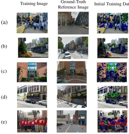
Figure 3.4: Initial training data generation. Positive and negative training examples are depicted in green and blue, respectively.
3.1.2 Predicting good features for geo-localization
In this section, we first outline our method for automatically generating the training examples. We then describe our classification model and the details of training procedure.
3.1.2.1 Automatic training data generation
λλ,,φφ
(d) Training features (b) Matching
⋮
⋮
Binary Classifier (Linear SVM) Retrieved Imagesλ ,φλ ,φ
⋮ (c) Retrieved images
λ�,φ�
(a) Training images (e) Bottom-up clustering (f) Bank of SVM classifiers
Green: Positive
Blue: Negative
False Positive Ground-Truth
⋮ ⋮
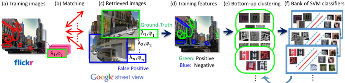
Figure 3.5: Overview of our training framework. For all training images that have GPS-tags (a), we retrieve top n images from the reference set (b-c). Positive labels are assigned to features that have higher matching score in the ground-truth reference image than in the falsely retrieved reference images, with a margin greater than thres. Negative labels are assigned in a similar manner (d). To handle noise and high intra-class variation, we use a bottom-up clustering technique, refining the positive set as well as training SVMs iteratively (e-f).
3.1.2.2 Closed-loop training of SVM classifiers
The automatic labeling approach above can sometimes generate contradictory labels for features with similar appearance. This commonly occurs in visual elements that appear on both transient and static objects. In Figure 3.4, for example, text on buses (b) and t-shirts (e) is assigned a negative label, while text on buildings and store signs (d) belongs to the positive set. A limited field-of-view overlap between a training image and a ground truth image can also lead to such contradictory labeling. Windows on the same building, for instance, can be assigned to different labels due to their visibility in the ground-truth reference image IGT. Such contradictory labeling on similar features limits the prediction accuracy.
On the other hand, there exists high intra-class variation in both the positive and negative classes: Windows have different appearances from text, for example, yet features from both appear in the same class. Training a single classifier over the entire data may be negatively affected by such intra-class variation.
To solve the problems of contradictory labeling and intra-class variation, we perform bottom-up clustering (Doersch et al., 2012) on the initial training feature set. By doing so, we obtain clusters of training examples whose appearances and labels are most consistent, as well as a bank of linear SVM classifiers that are trained within each cluster. Each training example constructs a cluster by finding k nearest neighbors in the training set. Redundant sets whose top ranked elements overlap with existing sets are eliminated. If a cluster has a high ratio of negative labels, the negative examples in that cluster are assigned to the final negative set N and the positive ones are discarded.
Figure 3.6: Top elements in the final clusters with a high ratio of positive labels. Each half row corresponds to different clusters.
classifiers whose weight vectors have a high cosine similarity with that of other classifiers as in (Juneja et al., 2013). Examples of top elements in Ci are shown in Figure 3.6. Figure 3.7 shows elements inN, which are aligned according to their initial clusters. Interestingly, although our approach makes no assumption on features that are useful for geo-localization, we can observe semantic relationships emerge through the learning process. Namely, windows, characteristic wall patterns, and letters on signage are detected as positive elements, while features from trees, people, car wheels, pavements, and edges are considered as negative elements.
Figure 3.7: Final negative set elements aligned according to their initial clusters. Each half row corresponds to different clusters.
Implementation details. Before comparing f(pt, IGT) and f(pt, IF P), we normalize the matching scores by multiplying max(1f) to compensate for a non-uniform distribution of features. For training and prediction, we separated features into three scale levels based on the size of the MSER, as we observed that the distribution of positive and negative PBVLAD features varies in different scales. The number of SVM classifiers used in each level were 35, 150, and 25, in an ascending order of the MSER size.
3.2 Experiments
We first evaluate our proposed pipeline with feature selection based on PBVLAD for image geo-localization. We quantitatively compare it with various baselines to demonstrate its efficacy. We also show qualitative results and failure cases to illustrate the performance of our method. Then, to further assess the benefit of our proposed PBVLAD, we evaluated it on a standard image retrieval benchmark.
3.2.1 Image Geo-localization
images that is used for the Pittsburgh portion of the reference set in the work of Zamir and Shah (2010). These images contain 8 overlapping perspective views extracted from the spherical panoramas in two different pitch directions, to capture both eye-level street views and the higher parts of the building in urban environments. This setting is similar to those used in (Doersch et al., 2012; Gronat et al., 2013; Torii et al., 2015b). The test image setIq was formed by 145 Internet collection images from the query set of Zamir and Shah (2010) with manually verified GPS-tags that are taken in Pittsburgh. The co-located GPS-tagged training image set It, comprising positive and negative training dataCi’s and N for learning, was downloaded from Flickr and consisted of 850 images that were successfully registered to the geographically nearby images in Ir through geometric verification.
Results. We compare the proportion of correctly localized images among a ranked list of the top n candidates. All of our results are without post-processing such as geometric re-ranking (Philbin et al., 2007). We consider an image to be localized if it is within 35m from the ground truth location. For a baseline, we compare with our implemented version of (Zamir and Shah, 2010). We also compare a variant of (Zamir and Shah, 2010) with SIFT feature selection by pre-trained linear SVM in a procedure similar to our selection of PBVLAD features (SIFT Select).
Figure 3.8 depicts how our systems with selected PBVLAD (PBVLAD Select) and all PBVLAD (PBVLAD All) consistently outperform the baseline methods. Feature selection is more successful in PBVLAD than SIFT. The performance of using selected features is consistently better than using all features in PBVLAD, whereas this behavior alternates when considering SIFT features.
Table 3.1: Proportion of correctly localized images at top 1
Method % Correct
PBVLAD All 64.83
PBVLAD Select 68.28
PBVLAD Random 33.38
PBVLAD Select{ 19.31
SIFT All (Zamir and Shah, 2010) 49.66
SIFT Select 46.90
Chance 0.20
5 10 15 20 25 30 35 40 45 50
40 50 60 70 80 90 100
Number of Candidates
Fraction of Correctly Localized Images (%)
PBVLAD Select PBVLAD All SIFT Select SIFT All
Figure 3.8: Geo-localization performance
of our selection mechanism, illustrating how simply selecting fewer features does not generally improve the performance. Moreover, we also tested with the features that are not selected by our framework (PBVLAD Select{) to illustrate how discarded features are in general detrimental to the geo-localization. The random chance of retrieving correct images is 0.2 %, which reflects difficulty posed by the dataset.
(a) (b) (c) (d) (e)
Figure 3.10: Qualitative comparison of retrieved image using selected PBVLAD and using all of the features. (a) Query image. (b) Heat map representation of the confidence of being a good feature. (c) Selected features (green:selected,blue:discarded). (c) The top retrieved image using selected
(a) (b) (c)
Figure 3.11: (a) Query image. (b) Heat map of maximum matching scores maxIr(f(pq, Ir)) of all features pq. (c) Confidence scores.
images despite partial occlusions and changes in viewpoint, illumination, and scale. Figure 3.10 depicts other examples where PBVLAD Select outperforms PBVLAD All.
We attribute the enhanced performance of PBVLAD-based retrieval to the increased discrimination power provided by aggregated features. Figure 3.11 (b) illustrates the maximum obtained feature similarity score for the features within a query image (a) w.r.t. the entire reference dataset. We can observe that PBVLAD features in foliage image regions are not highly matched to the reference set. Where individual SIFT features may have many similar features in the dataset, the analysis of their local ensembles is more discriminative. Moreover, our final predicted feature scores (c) illustrate how our framework discriminates good features prior to matching.
3.2.1.1 Failure cases
Query image Ground-truth Retrieved image
Figure 3.12: Failure cases. Retrieved images are more than 100m away from the ground-truth locations.
group members are missing. This could be alleviated by using spectral SIFT (Koutaki and Uchimura, 2014), or by only including keypoints detected within some scale range from the MSER region similar to (Chum et al., 2009).
3.2.2 PBVLAD for general image retrieval
Table 3.2: Comparative image retrieval performance of PBVLAD on the Oxford 5k dataset. The accuracy is measured by the mean Average Precision (mAP). All descriptors are uncom-pressed.
Descriptor # Vocabulary mAP
BoW (J´egou et al., 2012) 200,000 0.364 BoW (J´egou et al., 2012) 20,000 0.319 Fisher (J´egou et al., 2012) 64 0.317 VLAD (Eggert et al., 2014) 128 0.339
PBVLAD 128 0.369
Table 3.3: Retrieval performance of PBVLAD on Oxford 5k dataset, before and after the dimensionality reduction using PCA. The accuracy is measured by the mean Average Precision (mAP).
Full Dim Reduced
Dim 16384 8192 4096 2048 1024 mAP 0.369 0.364 0.334 0.264 0.210
3.3 Conclusion
CHAPTER 4: LEARNED CONTEXTUAL FEATURE REWEIGHTING FOR IMAGE GEO-LOCALIZATION
Visual image geo-localization has been an active research area for the past decade (Arandjelovi´c et al., 2016; Kim et al., 2015; Saurer et al., 2016; Taneja et al., 2014), owing to its wide range of applications including augmented reality (Middelberg et al., 2014), autonomous driving (Lim et al., 2012), adding and refining geo-tags in image collections (Hays and Efros, 2015; Zamir et al., 2014), large-scale 3D reconstruction (Crandall et al.,
2011), and photo editing (Zhang et al., 2014).
Finding regions of interest has long been of great interest in computer vision. Much research has been done in the areas of feature selection, attention, and saliency (Hou and Zhang, 2007; Yoo et al., 2015; Mnih et al., 2014). Because task-relevant information is not generally uniformly distributed throughout an image (Almahairi et al., 2015), focusing on “interesting” areas, as opposed to “irrelevant” or even “distracting” areas, can often achieve better performance (Shrivastava et al., 2011; Kim et al., 2015; Girshick et al., 2016). This is especially true for image geo-localization, where challenges come not only from photometric and geometric changes between the query and the database images, but also from confusing visual elements (Knopp et al., 2010). For instance, features extracted from transient objects such as pedestrians and trees, or ubiquitous objects, like vehicles and fences, can introduce misleading cues into the geo-localization process.
feature map
conv layers
input image
Contextual Reweighting
Network
(a) (c)
(b)
reweighted features
CRN
image representation
Figure 4.1: Image representation with contextual feature reweighting. (a) A contextual reweighting network takes convolutional features of a deep CNN as input to produce a spatial weighting mask (b) based on the learned contexts. The mask is used for weighted aggregation of input features to produce the representation of the input image (c).
a data-driven notion of “good” features as features that offer relatively high matching score to correct locations.
However, these approaches focus their analysis on individual local features in general. What is often overlooked is that a feature’s usefulness depends largely on the context in the scene. For example, signage on buildings is useful for geo-localization, while signage on buses and t-shirts is misleading. There have been attempts to use top-down information such as semantic segmentation to restrict features to man-made structures (Mousavian and Koˇsecka, 2015), or repetitive structure detection to avoid over-counting of visual words in the bag-of-words representation (Torii et al., 2015b). We point out that such supervised priors are limited and do not capture all relevant context about which regions to focus on for image geo-localization.
(Fig. 4.1 (a)). The CRN takes the feature maps of the base convolutional layers and estimates a weight for each feature based on its surrounding region (Fig. 4.1 (b)). By feature, we mean a column of activations at each spatial location of the feature maps. These weights are then applied to each feature as they are aggregated to produce an overall image representation.
We cast the image geo-localization problem as an image retrieval task and optimize the network with a triplet ranking loss based on the generated image representations. As a result, task-relevant contexts are discovered in an unsupervised manner, as the network learns in which context certain features should be emphasized or suppressed to better produce the spatial weighting, even though no ground-truth for the weighting nor the context information is provided. Visualizations of these learned contexts illustrate that the discovered contextual information contains rich high-level information that is not restricted to semantic cues, such as different types of buildings, vehicles, vegetation, and ground, but includes structural cues like lattice structure, different perspectives of buildings, and architectural styles.
Our training pipeline requires no training labels other than image geo-tags, which are commonly available on Internet photo collections such as Flickr. We use geometric verification to confirm the relationship between two views, then take the convex hull of matched inlier points to generate positive image pairs for training. In addition, we introduce efficient hard negative mining for image geo-localization, which can be seen as mimicking the image geo-localization process within a training batch.
To summarize, the innovations of this work are as follows: (1) We propose a novel end-to-end, fully-convolutional CNN for learning image representations that integrates context-aware feature reweighting. In particular, we introduce a contextual reweighting network that predicts weights for each region in the feature map based on its context. We experimentally validate that our pipeline significantly boosts the performance of the state-of-the-art methods. (2) We also show that unsupervised context discovery is achieved as a byproduct of training
Feature Map ( W x H x D )
Context Filter Output ( W x H x P ) Contextual Reweighting Mask
( W x H )
Weighted Sum
Multiscale Context Filters
( npx npx D )
Figure 4.2: Contextual Reweighting Network. For each 1×1×D convolutional feature, multi-scale contextual information is captured by P context filters with different window sizes (np×np×D). The filter output is then accumulated with learned weights to produce a reweighting value for the feature in question.
image geo-tags are required to automatically generate training data, with an efficient hard negative mining solution for image geo-localization.
4.1 Method
In this section, we first describe our model for learning image representations that integrate contextual reweighting of features (Sec. 4.1.1). We then illustrate our learning objective and the overall training process (Sec. 4.1.2).
4.1.1 The Contextual Reweighting Network