Education Corner
An introduction to g methods
Ashley I Naimi
1*, Stephen R Cole
2and Edward H Kennedy
31
Department of Epidemiology, University of Pittsburgh,
2Department of Epidemiology, University of
North Carolina at Chapel Hill and
3Department of Statistics, Carnegie Mellon University
*Corresponding author. Department of Epidemiology University of Pittsburgh 130 DeSoto Street 503 Parran Hall Pittsburgh, PA 15261 [email protected]
Accepted 17 October 2016
Abstract
Robins’ generalized methods (g methods) provide consistent estimates of contrasts (e.g.
differences, ratios) of potential outcomes under a less restrictive set of identification
con-ditions than do standard regression methods (e.g. linear, logistic, Cox regression).
Uptake of g methods by epidemiologists has been hampered by limitations in
under-standing both conceptual and technical details. We present a simple worked example
that illustrates basic concepts, while minimizing technical complications.
Key words: G Methods; Marginal Structural Model; Structural Nested Model; G Formula; Inverse Probability Weighting; G Estimation; Monte Carlo Estimation
Robins’ g methods enable the identification and estimation of the effects of generalized treatment, exposure, or inter-vention plans. G methods are a family of methods that include the g formula, marginal structural models, and structural nested models. They provide consistent estimates of contrasts (e.g. differences, ratios) of average potential
outcomes under a less restrictive set of identification condi-tions than standard regression methods (e.g. linear, logis-tic, Cox regression).1 Specifically, standard regression
requires no feedback between time-varying treatments and time-varying confounders, while g methods do not. Robins and Hernan1 have provided a technically comprehensive
Key Messages
• G methods include inverse probability weighted marginal structural models, g estimation of a structural nested
model, and the g formula.
• G methods estimate contrasts of potential outcomes under a less restrictive set of assumptions than standard
regres-sion methods.
• Inverse probability weighting generates a pseudo-population in which exposures are independent of confounders,
enabling estimation of marginal structural model parameters.
• G estimation exploits the conditional independence between the exposure and potential outcomes to estimate
struc-tural nested model parameters.
• The g formula models the joint density of the observed data to generate potential outcomes under different exposure
scenarios.
VCThe Author 2016; all rights reserved. Published by Oxford University Press on behalf of the International Epidemiological Association 756
doi: 10.1093/ije/dyw323 Advance Access Publication Date: 30 December 2016 Education Corner
worked example of each of the three g methods. Here, we present a corresponding worked example that illustrates the need for and use of g methods, while minimizing tech-nical details.
Example
Our research question concerns the effect of treatment for HIV on CD4 count.Table 1presents data from a hypothet-ical observational cohort study (A¼1 for treated, A¼0 otherwise). Treatment is measured at baseline (A0) and once during follow up (A1). The sole covariate is elevated HIV viral load (Z¼1 for those with > 200 copies/ml,
Z¼0 otherwise), which is constant by design at baseline (Z0¼1) and measured once during follow up just prior to the second treatment (Z1). The outcome is CD4 count measured at the end of follow up in units of cells/mm3. The
CD4 outcome in Table 1 is summarized (averaged) over the participants at each level of the treatments and covari-ate. The number of participants is provided in the right-most column ofTable 1. In this hypothetical study of one million participants we ignore random error and focus on identifying the parameters defining our causal effect of interest, which we describe next.
Based onFigure 1, the average outcome in our simple data generating structure may be composed of several parts: the effects ofA0,Z1, andA1; the two-way interac-tions betweenA0andZ1,A0andA1, andA1andZ1; and the three-way interaction betweenA0,Z1, andA1. These components (some whose magnitudes may be zero) can be used to “build up” a contrast of substantive interest. Here, we focus on the average causal effect of always taking treatment (a0¼1;a1¼1) compared to never taking treat-ment (a0¼0;a1¼0),
w¼EðYa0¼1;a1¼1Þ EðYa0¼0;a1¼0Þ ¼EðYa0¼1;a1¼1Ya0¼0;a1¼0Þ;
where expectationsEðÞare taken with respect to the target population from which our sample is a random draw. This average causal effect consists of the joint effect ofA0and
A1onY.2Here,Ya0;a1represents a potential outcome value that would have been observed had the exposures been set to specific levelsa0anda1. This potential outcome is dis-tinct from the observed (or actual) outcome.
This average causal effectw¼EðYa0;a1Y0;0Þis a
mar-ginal effect because it averages (or marginalizes) over all individual-level effects in the population. We can write this effect as EðYa0;a1Y0;0Þ ¼w
0a0þw1a1þw2a0a1, which states that our average causal effectwmay be composed of two exposure main effects (e.g.,w0andw1) and their two-way interaction (w2). This marginal effectwis indifferent to whether theA1component (w1þw2) is modified byZ1: whether such effect modification is present or absent, the marginal effect represents a meaningful answer to the ques-tion: what is the effect of A0 and A1 in the entire population?
Alternatively, we may wish to estimate this effect condi-tionalon certain values of another covariate. A conditional effect would arise if, for example, one was specifically interested in effect measure modification by Z1. When properly modeled, this conditional effect represents a meaningful answer to the question: what is the effect ofA0 and A1 in those who receive Z1¼1 versus those who receive Z1¼0? Modeling such effect measure modifica-tion by time-varying covariates is the fundamental issue that distinguishes marginal structural from structural nested models. We thus return to this issue later. For sim-plicity, we define our effect of interest as w¼w0þw1þw2, and we explore a data example with no effect modification by time-varying confounders.
Assumptions
Our average causal effect is defined as a function of two averages that would be observed if everybody in the popu-lation were exposed (or unexposed) at both time points. Table 1. Prospective study data illustrating the number of
subjects (N) within each possible combination of treatment at
time 0 (A0), HIV viral load just prior to the second round of
treatment (Z1), and treatment status for the 2nd round of
treatment (A1). The outcome column (Y) corresponds to the
mean ofYwithin levels ofA0,Z1,A1. Note that HIV viral load
at baseline is high (Z0¼1) for everyone by design
A0 Z1 A1 Y N
0 0 0 87.29 209,271
0 0 1 112.11 93,779
0 1 0 119.65 60,654
0 1 1 144.84 136,293
1 0 0 105.28 134,781
1 0 1 130.18 60,789
1 1 0 137.72 93,903
1 1 1 162.83 210,527
Figure 1. Causal diagram representing the relation between anti-retro-viral treatment at time 0 (A0), HIV viral load just prior to the second
round of treatment (Z1), anti-retroviral treatment status at time 1 (A1),
the CD4 count measured at the end of follow-up (Y), and an unmeas-ured common cause (U) of HIV viral load and CD4.
Yet we cannot directly acquire information on these aver-ages because in any given sample, some individuals will be unexposed (or exposed). Part of our task therefore involves justifying use of averages among subsets of the population as what would be observed in the whole population. This is accomplished by making three main assumptions.
Counterfactual consistency3 allows us to equate
observed outcomes among those who received a certain exposure value to the potential outcomes that would be observed under the same exposure value:
EðYjA0¼a0;A1¼a1Þ ¼EðYa0;a1jA0¼a0;A1¼a1Þ
The status of this assumption remains unaffected by the choice of analytic method (e.g., standard regression versus g methods). Rather, this assumption’s validity depends on the nature of the exposure assignment mechanism.4Under counterfactual consistency, we partially identify our aver-age causal effect.
Next, we assume exchangeability.5 Exchangeability implies that the potential outcomes under exposuresa0and
a1 (denoted Ya0;a1) are independent of the actual (or observed) exposuresA0and A1. We make this exchange-ability assumption within levels of past covariate values (conditional) and at each time point separately (sequential):
EðYa0;a1jA
1;Z1;A0Þ ¼EðYa0;a1jZ1;A0Þ; and (1)
EðYa0;a1jA
0Þ ¼EðYa0;a1Þ: (2) This sequential conditional exchangeability assumption would hold if there were no uncontrolled confounding and no selection bias. Equation 1 says that, within levels of prior viral load (Z1) and a given treatment levelA0,Ya0;a1 does not depend on the assigned values ofA1.Equation 2 says thatYa0;a1 does not depend on the assigned values of
A0. Note the correspondence between these two equations and the causal diagram: because inFigure 1,Z1is a com-mon cause ofA1andY, the assumption inequation 1must be made conditional onZ1. Failing to condition forZ1will result in uncontrolled confounding of the effect ofA1, and thus a dependence between the actual A1 value and the potential outcome. However, adjusting forZ1using stand-ard methods (restriction, stratification, matching, or condi-tioning in a linear regression model) would block part of the effect fromA0 throughZ1, and potentially lead to a collider bias of the effect ofA0throughU.6This is the cen-tral challenge that g methods were developed to address.
The third assumption, known as positivity,7requires 0 < P
ðA1¼1jZ1¼z1;A0¼a0Þ < 1 and 0 < PðA0¼1Þ < 1. Furthermore, this assumption must hold for all values ofa0 and z1 where PðA0¼a0;Z1¼z1Þ>0. This latter condi-tion is required so that effects are not defined in strata ofa0
andz1 that do not exist. Positivity is met when there are exposed and unexposed individuals within all confounder and prior exposure levels, which can be evaluated empirically.
Under these three assumptions, our hypothetical obser-vational study can be likened to a sequentially randomized trial in which the exposure was randomized at baseline, and randomized again at time 1 with a probability that depends on Z1. Under these assumptions, g methods can be used to estimate counterfactual quantities with observa-tional data. In the Supplementary Material, we provide SAS code (SAS Institue, Cary, NC) in which standard regression and all three g methods are fit to the hypotheti-cal data inTable 1.
Results
Standard Methods
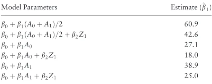
Table 2presents results from fitting a number of standard linear regression models to the data inTable 1. In the first model,^b¼60:9 cells/mm3is the crude difference in mean CD4 count for the always treated compared to the never treated. In model two, b^¼42:6 cells/mm3 is the Z1 -adjusted difference in mean CD4 count for the same con-trast. Other model results are provided in Table 2, and more could be entertained.
Table 3presents the results from fitting all three g meth-ods to the data inTable 1. The marginal structural model resulted inw^ ¼50:0 cells/mm3. The g formula resulted in ^
w¼50:0 cells/mm3. Finally, the structural nested model
resulted inw^ ¼50:0 cells/mm3. Next we discuss how we obtained these results.
G Methods
The g formula can be used to estimate the average CD4 level that would be observed in the population under a given treatment plan. To implement the approach, we start with a mathematical representation of the data generating
Table 2. A selection of regression models fit to the data in
Table 1, and parameter estimates for various exposure
contrasts
Model Parameters Estimate (^b1)
b0þb1ðA0þA1Þ=2 60.9
b0þb1ðA0þA1Þ=2þb2Z1 42.6
b0þb1A0 27.1
b0þb1A0þb2Z1 18.0
b0þb1A1 38.9
b0þb1A1þb2Z1 25.0
mechanism for all variables inTable 1. We refer to this as the joint density of the observed data. We factor the joint density in a way that respects the temporal ordering of the data by conditioning each variable on its history. For example, iffðÞrepresents the probability density function, then by the definition of conditional probabilities8ðp36Þwe
can factor this joint density as
fðy;a1;z1;a0Þ ¼fðyja1;z1;a0ÞPðA1 ¼a1jZ1¼z1;A0¼a0Þ
PðZ1¼z1jA0¼a0ÞPðA0¼a0Þ:
Our interest lies in the marginal mean ofYthat would be observed ifA0andA1were set to some valuesa0anda1, respectively. To obtain this expectation, we perform two mathematical operations on the factored joint density. The first is the well-known expectation operator,8ðp47Þ which
allows us to write the conditional mean ofYin terms of its conditional density. The second is the law of total proba-bility,8ðp12Þwhich allows us to marginalize over the
distri-bution ofA1,Z1andA0, yielding the marginal mean ofY:
EðYÞ ¼ X
a1;z1;a0
EðYjA1¼a1; Z1¼z1;A0¼a0Þ
PðA1¼a1jZ1¼z1;A0¼a0Þ
PðZ1¼z1jA0¼a0ÞPðA0¼a0Þ:
We can now modify this equation to yield the average of potential outcomes that would be observed after inter-vening on the exposure [enabling us to drop out the terms forPðA1¼a1jZ1¼z1;A0¼a0ÞandPðA0¼a0Þ], yielding
EðYa0;a1Þ ¼X
z1
EðYjA1¼a1;Z1¼z1;A0¼a0Þ
PðZ1¼z1jA0¼a0Þ:
This equation is the g formula; its proof, given in the Supplementary Material, follows from the three identify-ing assumptions. In our simple scenario, the expectation
EðY0;0Þ can be calculated by summing the mean CD4 count in the never treated withZ1¼1 (weighted by the proportion of people withZ1¼1 in theA0¼0 stratum)
and the mean CD4 count in the never treated withZ1¼0 (weighted by the proportion of people withZ1¼0 in the
A0¼0 stratum). Weighting the observed outcome’s con-ditional expectation by the concon-ditional probability that
Z1¼z1 enables us to account for the fact that Z1 is affected byA0, but also confounds the effect ofA1onY. Computing this expectation’s value yields a result of
^
EðY0;0Þ ¼100:0, where we use E^ to denote a sample, rather than a population average, and with the under-standing thatE^ðY0;0Þ is equal to the g formula with A
0
¼A1¼0 (since the potential outcomes Y0;0 are not directly observed). We repeat the process to obtain the corresponding value for treated at time 0 only:
^
EðY1;0Þ ¼125:0; treated at time 1 only:E^ðY0;1Þ ¼125:0; and always treated:E^ðY1;1Þ ¼150:0. Thus,w^
GF¼150:0
100:0¼50:0, which is the average causal effect of treat-ment on CD4 cell count.
This approach to computing the value of the g formula is referred to as nonparametric maximum likelihood esti-mation. Several authors9–13 demonstrate how simulation from parametric regression models can yield a g formula estimator, which is often required in typical population-health studies with many covariates.
Modeling each component of the joint density of the observed data (including the probability thatZ1¼z1) can lead to bias if any of these models are mis-specified. To compute the expectations of interest, we can instead spec-ify a single model that targets our average causal effect, and avoid unnecessary modeling. Marginal structural mod-els map a marginal summary(e.g., average) of potential outcomes to the treatment and parameter of interest w.
Unlike the g formula, they do not require a model for
PðZ1¼z1jA0¼a0Þ. Additionally, as we show in the Supplementary Material, while they cannot model it directly, they are indifferent to whether time-varying effect modification is present or absent. Because our interest lies in the marginal contrast of outcomes under always versus never treated conditions, our marginal structural model for the effect of A can be written as EðYa0;a1Þ ¼b
0þw0a0
þw1a1þw2a0a1, whereb0¼EðY0;0Þis a (nuisance) inter-cept parameter, andw¼EðY1;1Y0;0Þ ¼ ðw
0þw1þw2Þ is the effect of interest.
Inverse probability weighting can be used estimate mar-ginal structural model parameters (proofs are provided in theSupplementary Material). To estimatewusing inverse probability weighted regression, we first obtain the pre-dicted probabilities of the observed treatments. In our example data, there are two possibleA1values (exposed, unexposed) for each of the four levels in Z1 and A0. Additionally, there are two possible A0 values (exposed, unexposed) overall. This leads to four possible exposure regimes: never treat, treat early only, treat late only, and Table 3. G methods and corresponding estimates comparing
contrasts quantifying always exposed versus never exposed
scenarios fit to data inTable 1
G Method w^a
G Formula 50.0
IP-weighted marginal structural model 50.0
G Estimated Structural Nested Model 50.0
aw¼EðY1;1Y0;0Þ
always treat. For eachZ1value, we require the predicted probability of the exposure that was actually received. These probabilities are computed by calculating the appro-priate proportions of subjects inTable 1. Because there are no variables that affectA0, this probability is 0.5 for all individuals in the sample. Furthermore, in our exampleA1 is not affected byA0(Figure 1). Thus, theZ1specific prob-abilities ofA1are constant across levels ofA0. In settings where A0 affects A1, the Z1 specific probabilities of A1 would vary across levels ofA0.
In the stratum defined byZ1¼1, the predicted proba-bilities ofA1¼0 andA1¼1 are 0.308 and 0.692, respec-tively. For example, ð210;527þ136;293Þ=ð210;527 þ136;293þ93;903þ60;654Þ ¼0:692. Thus, the prob-abilities for each treatment combination are: 0:50:308 ¼0:155 (never treated), 0:50:308¼0:155 (treated early only), 0:50:692¼0:346 (treated late only), and 0:50:692¼0:346 (always treated). Dividing the mar-ginal probability of each exposure category (not stratified byZ1) by these stratum specific probabilities gives stabi-lized weights of 1.617, 1.617, 0.725, and 0.725, respec-tively. For example, the never treated weight is ð0:50:501Þ=ð0:50:308Þ ¼1:617. The same approach is taken to obtain predicted probabilities and stabilized weights in the stratum defined byZ1¼0. The weights and weighted data are provided inTable 4.
Fitting this model in the weighted data given inTable 4 provides the inverse-probability weighted estimates ½w^0IP¼25:0;w^1IP¼25:0;w^2IP¼0:0, thus yielding ^
wIP¼50:0.
Weighting the observed data by the inverse of the prob-ability of the observed exposure yields a “pseudo-pop-ulation” (Table 4) in which treatment at the second time point (A1) is no longer related to (and is thus no longer confounded by) viral load just prior to the second time point (Z1). Thus, weighting a conditional regression model for the outcome by the inverse probability of treatment enables us to account for the fact thatZ1both confounds
A1and is affected byA0.
Structural nested models map a conditional contrast of potential outcomes to the treatment, within nested sub-groups of individuals defined by levels ofA1,Z1, andA0. Our struc-tural nested model can be written with two equations as
EðYa0;a1Ya0;0jA
0¼a0;Z1¼z1;A1¼a1Þ
¼a1ðw1þw2a0þw3z1þw4a0z1Þ
EðYa0;0Y0;0jA
0¼a0Þ ¼w0a0
Note this model introduces two additional parameters:w3 for the two-way interaction betweena1andz1, andw4for the three-way interaction betweena1,z1, and a0. Indeed, the ability to explicitly quantify interactions between time-varying exposures and time-time-varying covariates (which can-not be modeled via standard marginal structural models) is a major strength of structural nested models when effect modification is of interest.1To simplify our exposition, we
set ðw3;w4Þ ¼ ð0;0Þ in our data example, allowing us to
drop thew3z1andw4a0z1terms from the model. In effect, this renders our structural nested mean model equivalent to a semi-parametric marginal structural model. In the Supplementary Material, we explain how marginal struc-tural and strucstruc-tural nested models each relate to time-varying interactions in more detail.
We can now use gestimation to estimateðw0;w1;w2Þin the above structural nested model. Gestimation is based on solving equations that directly result from the sequential conditional exchangeability assumptions in (1) and (2), combined with assumptions implied by the structural nested model. If, at each time point, the exposure is condi-tionally independent of the potential outcomes (sequential exchangeability) then the conditional covariance between the exposure and potential outcomes is zero.14 Formally, these conditional independence relations can be written as:
0¼CovðYa0;0;A
1jZ1;A0Þ
¼CovðY0;0;A 0Þ
where CovðÞis the well-known covariance formula.8ðp52Þ
These equalities are of little direct use for estimation, though, as they contain unobserved potential outcomes and are not yet functions of the parameters of interest. However, by counterfactual consistency and the structural nested model, we can replace these unknowns with quanti-ties estimable from the data.
Specifically, as we prove in the Supplementary Material, the structural nested model, together with exchangeability and counterfactual consistency imply that we can replace the potential outcomesYa0;0andY0;0in the above covariance formulas with their values derived from the structural nested model, yielding:
Table 4. Stabilized inverse probability weights and
Pseudo-population obtained by using inverse probability weights
A0 Z1 A1 Y sw PseudoN
0 0 0 87.23 0.72 151222.84
0 0 1 112.23 1.62 151680.46
0 1 0 119.79 1.62 98110.06
0 1 1 144.78 0.72 98789.40
1 0 0 105.25 0.72 97395.08
1 0 1 130.25 1.62 98321.62
1 1 0 137.80 1.62 151884.02
1 1 1 162.80 0.72 152596.51
0¼CovfYA1ðw1þw2A0Þ;A1jZ1;A0g
¼CovfYA1ðw1þw2A0Þ w0A0;A0g:
We provide an intuitive explanation for this substitu-tion in the Supplementary Material. We also show how these covariance relations yield three equations that can be used to solve each of the unknowns in the above structural nested model (w0;w1;w2). Two of the three equations yield the following g estimators:
^ w1GE ¼
^
E½ð1A0ÞYfA1E^ðA1jZ1;A0Þg
^
E½ð1A0ÞA1fA1E^ðA1jZ1;A0Þg
^ w1GEþ
^ w2GE ¼
^
E½A0YfA1E^ðA1jZ1;A0Þg
^
E½A0A1fA1E^ðA1jZ1;A0Þg
Note that to solve these equations we need to model
EðA1jZ1;A0Þ, which in practice we might assume can be correctly specified as the predicted values from a logistic model forA1. In our simple setting, the correctness of this model is guaranteed by saturating it (i.e., conditioning the model onZ1,A0and their interaction).
As we show in theSupplementary Material, implement-ing these equations in software can be easily done usimplement-ing either an instrumental variables (i.e., two-stage least squares) estimator, or ordinary least squares.
Once the above parameters are estimated, the next step is to subtract the effect ofA1andA1A0 fromYto obtain
~
Y¼Yw^1GEA1
^
w2GEA1A0. We can then solve for the
last parameter using a sample version of the third g estima-tion equality, yielding our final estimator and completing the procedure:
^
w0GE ¼ E^½Y~fA0E^ðA0Þg ^
E½A0fA0E^ðA0Þg :
Again the above estimator can be implemented using an instrumental variable or ordinary least squares estimator. Implementing this procedure in our example data, we obtain ½w0GE ¼25:0;w1GE ¼25:0;w2GE¼0:0, thus yield-ingwGE¼50:0.
The potential outcome under no treatment can be thought of as a given subject’s baseline prognosis: in our setting, individuals with poor baseline prognosis will have low CD4 levels, no matter what their treatment status may be. In the absence of confounding or selection bias, one expects this baseline prognosis to be independent of treatment status. G estimation exploits this independence by assuming no uncontrolled confounding (conditional on measured confounders), and assigning values tow^GE that render the potential outcomes independent of the
exposure. However, assigning the correct values tow^
GE
depends on there being no confounding or selection bias.
Discussion
Having constructed these data using the causal diagram shown inFigure 1, we know the true effect of combined treatment is indeed 50 cells/mm3 (25 cells/mm3 for each exposure main effect) as well approximated by all three g methods, but not by any of the standard regression models we fit, with one exception. The final standard result pre-sented inTable 2correctly estimates the effect of the sec-ond treatment (an effect of 25 cells/mm3), as would be expected from the causal diagram.
For the past several years, we have used the foregoing simple example to initiate epidemiologists to g methods with some success. Once having studied this simple exam-ple in detail, we recommend working through more com-prehensive examples by Robins and Hernan1and Hernan
and Robins.16 A recent tutorial2 may then be of further use. G methods are becoming more common in epidemio-logic research.17We hope this commentary facilitates the process of better understanding these useful methods.
Funding
Stephen Cole was supported in part by NIH grants R01AI100654, R24AI067039, U01AI103390, and P30AI50410.
Acknowledgements
The authors thank Miguel A. Hernan, Jessica R. Young, Ian Shrier and an anonymous reviewer for expert advice.
Conflicts of interest:None declared.
References
1. Robins J and Hernan M. Estimation of the causal effects of time-varying exposures. In: Fitzmaurice G, Davidian M, Verbeke G, and Molenberghs G (Eds.) Advances in Longitudinal Data Analysis. Boca Raton, FL: Chapman & Hall. 2009; 553–599. 2. Daniel R, Cousens S, De Stavola B, Kenward MG, and Sterne
JAC. Methods for dealing with time-dependent confounding.
Stat Med2013;32:1584–618.
3. Cole SR and Frangakis CE. The consistency statement in causal inference: a definition or an assumption?Epidemiol2009;20:3–5. 4. VanderWeele TJ and Hernan MA. Causal inference under multiple
versions of treatment.Journal of Causal Inference2013;1:1–20. 5. Greenland S and Robins JM. Identifiability, exchangeability, and
epidemiological confounding. Int J Epidemiol 1986;
15(3):413–19.
6. Cole SR, Platt RW, Schisterman EFet al. Illustrating bias due to conditioning on a collider.Int J Epidemiol2010;39:417–420. 7. Westreich D and Cole SR. Invited commentary: Positivity in
practice.Am J Epidemiol2010;171:674–677.
8. Wasserman L.All of Statistics: A Concise Course in Statistical Inference. New York, NY: Springer, 2005.
9. Taubman SL, Robins JM, Mittleman MA, and Hernan MA. Intervening on risk factors for coronary heart disease: an applica-tion of the parametric g-formula. Int J Epidemiol 2009;
38:1599–611.
10. Westreich D, Cole SR, Young JGet al. The parametric g-formula to estimate the effect of highly active antiretroviral therapy on in-cident aids or death.Stat Med2012;31:2000–2009.
11. Cole SR, Richardson DB, Chu H, and Naimi AI. Analysis of oc-cupational asbestos exposure and lung cancer mortality using the g formula.Am J Epidemiol2013;177:989–996.
12. Keil A, Edwards JK, Richardson DB, Naimi AI, and Cole SR. The parametric g-formula for time-to-event data: to-wards intuition with a worked example. Epidemiol 2014;
25:889–97.
13. Edwards JK, McGrath L, Buckley JP and Schubauer-Berigan, MKet al. Occupational radon exposure and lung cancer mortal-ity: Estimating intervention effects using the parametric g-for-mula.Epidemiol2014;25:829–34.
14. Vansteelandt S and Joffe M. Structural nested models and g-esti-mation: The partially realized promise. Statist Sci 2014;
29:707–731.
15. Robins JM, Mark SD, and Newey WK. Estimating exposure ef-fects by modelling the expectation of exposure conditional on confounders.Biometrics1992;48:479–95.
16. Hernan MA and Robins J. Causal Inference. Forthcoming. Chapman/Hall, http://www.hsph.harvard.edu/miguel-hernan/ causal-inference-book/, accessed 14 Oct 2016.
17. Suarez D, Borras R, and Basagana X. Differences between marginal structural models and conventional models in their exposure effect estimates: a systematic review.Epidemiol2011;22:586–588.