(will be inserted by the editor)
Relational Data Factorization
Sergey Paramonov · Matthijs van Leeuwen ·
Luc De Raedt
Received: date / Accepted: date
Abstract Motivated by an analogy with matrix factorization, we introduce the prob-lem of factorizing relational data. In matrix factorization, one is given a matrix and has to factorize it as a product of other matrices. In relational data factorization (ReDF), the task is to factorize a given relation as a conjunctive query over other relations, i.e., as a combination of natural join operations. Given a conjunctive query and the input relation, the problem is to compute theextensionsof the relations used in the query. Thus, relational data factorization is a relational analog of matrix fac-torization; it is also a forminversequerying as one has to compute the relations in the query from the result of the query. The result of relational data factorization is neither necessarily unique nor required to be a lossless decomposition of the origi-nal relation. Therefore, constraints can be imposed on the desired factorization and a scoring function is used to determine its quality (often similarity to the original data). Relational data factorization is thus a constraint satisfaction and optimization prob-lem. We show how answer set programming can be used for solving relational data factorization problems.
Keywords Answer Set Programming·Inductive Logic Programming·Pattern Mining·Relational Data·Factorization·Data Mining·Declarative Modeling
Sergey Paramonov
Machine Learning, Department of Computer Science, KU Leuven, Leuven, Belgium E-mail: [email protected]
Matthijs van Leeuwen
Machine Learning, Department of Computer Science, KU Leuven, Leuven, Belgium and Leiden Institute of Advanced Computer Science, Leiden University, Leiden, the Netherlands E-mail: [email protected]
Luc De Raedt
1 Introduction
The fields of data mining and machine learning have contributed numerous effective and highly optimized algorithms for analyzing data. However, this focus on efficiency and scalability has come at the cost of generality. Indeed, while the algorithms are highly effective, their application range is often very restricted, and the algorithms are typically hard to change and adapt even to small variations on the problem definition. This observation has led to an interest in declarative methods for data mining and machine learning in which the focus lies on the use of expressive models that can capture a wide range of different problem settings and that can then be solved using off-the-shelf constraint solving technology; see Guns et al (2013a); De Raedt (2012); Arimura et al (2012); De Raedt (2015).
Motivated by this quest for more general and generic data analysis approaches, the present paper introduces the problem of relational data factorization (ReDF). ReDF is inspired by matrix factorization, one of the most popular techniques in ma-chine learning and data mining for which many variants have been studied, such as non-negative, singular value and Boolean matrix factorization. In matrix factoriza-tion, one is given ann×mmatrixA, and the problem is to rewrite it as the product of some other matrices, e.g., the product of ann×kmatrixBandk×mmatrixC such thatAi,j=PkBi,k·Ck,j. In relational data factorization, one is given a
rela-tion (i.e., a set of tuples over the same attributes) and asked to to rewrite it in terms of other relations. Consider, for instance, a relationsells(Company, Part, Project), stat-ing that companies sell particular parts to particular projects. While it is well-known that ternary relations, in general, can not be rewritten as the join of three binary rela-tions (Heath, 1971; Jones et al, 1996)1, we might be interested in an approximation of the ternary relation. That is, we might approximatesells(Company, Part, Project)by the queryoffers(Company,Part), needs(Project, Part), deliversto(Company, Project)
(we follow logic programming notation, where the same variable name denotes a nat-ural join). The question is then how to determine the extensions for the relations of-fers,needs, anddelivers. The found solution will generally be imperfect, so in ReDF we want to find the best approximation w.r.t. a scoring function and we allow the user to specify hard constraints. In the example these might specify, e.g., that only tuples in the target relationsellsmay be derivable from the query.
In this paper, we develop a modeling and solving approach for ReDF using an-swer set programming (ASP) (Brewka et al, 2011). This is realized by showing for a number of ReDF problems how they can be tackled with ASP. This leads to the identification of constraints and scoring functions, which we then abstract to an even higher-level declarative language. We show that the resulting ReDF framework is general and generic and is in line with the declarative modeling approach to ma-chine learning and data mining as 1) it allows one to easily specify and solve a wide range of well-known data analysis problems (such as tiling, Boolean matrix factor-ization, discriminative pattern mining, matrix block diagonalfactor-ization, etcetera), 2) it is effective for prototyping such tasks (as we show in our experiments), even though it
1Heath Theorem: a relationR(x, y, z)satisfying a functional dependencyx → ycan always be
cannot yet compete with optimized special purpose algorithms in terms of efficiency, and 3) the constraints and optimization criteria are specified in a declarative and flex-ible manner. Translating problem definitions in the ReDF framework to ASP models is straightforward, and small changes in the problem definitions generally result in small changes in the model.
Relational data factorization is a form of relational learning. That is, it is a re-lational analog of matrix factorization and is therefore relevant to inductive logic programming (Muggleton and De Raedt, 1994; De Raedt, 2008) and can also be seen as a form of large-scale abduction (Denecker and Kakas, 2002). Moreover, the solu-tion techniques that we adopt are based on answer set programming, which has also been adopted in some recent works and methods on inductive logic programming (Paramonov et al, 2015; J¨arvisalo, 2011). The implementation techniques we employ may also be used in more traditional inductive logic programming settings.
This paper is structured as follows. Section 2 introduces the formal ReDF frame-work. Section 3 introduces ASP. Section 4 shows how a wide range of data mining problems can be expressed as ReDF problems. Section 5 introduces some novel lems that the framework can express. Section 6 discusses the encoding of the prob-lems into ASP, while Section 7 reports on the experimental evaluation. In Section 8 we discuss related work, and we formulate some conclusions and directions for future work in Section 9.
2 Relational Data Factorization
Before we formalize the ReDF problem and approach in its full generality, we il-lustrate Relational Data Factorization on thesells(Company, Part, Project)example from the Introduction.
2.1 An example
Assume we are given 1) a set of tuples for the database relationsells(Company, Part, Project), 2) a definite shapeclause defining the predicate approx(Company, Part, Project), e.g.,
approx (Com, Pa, Proj)←offers(Com, Pa), needs(Proj, Pa), deliversto(Com, Proj),
which should approximate the database relation sells(Company, Part, Project) in terms of the (unknown) relations offers(Company, Part), needs(Project, Part) and
deliversto(Com, Project), and 3) anerrorfunctionerror(approx,sells)that measures how different the database predicate and its approximation are, e.g., the number of tuples that is one in relation but not in the other. Then, the goal is to find sets of tuples for the unknown relations that minimize theerror.
2.2 Problem statement
Using a logic programming formalism, we generalize the above example into the following ReDF problem statement.
Given:
• a datasetD: a set of ground facts for target predicatedb;
• a factorization shapeQ:approx( ¯T)←q1( ¯T1), . . . , qk( ¯Tk), where theqiare
fac-tors and theT¯idenote tuples of variables;
• a set of constraintsC;
• anerrorfunction measuring difference between two predicates (i.e., between the corresponding sets of ground facts);
Find: the set of ground factsF for the factorsqi that minimizeserror(approx,db)
and for whichQ∪F∪Dsatisfies all constraints inC.
The factorization shape is a single non-recursive rule definingapprox, the approx-imation of the target predicatedb, where the predicates in the body are the factors. If a variable occurs in a body atomT¯iand not inT¯(the head), then it is calledlatent.
The task is to find a setF of ground facts defining the factorsqi. Furthermore, each
such setFuniquely determines a set of facts forapprox. Notice that if a predicateqi
is already known and defined, then the task simplifies.
As in matrix factorization, it is quite likely that a perfect solution, witherror= 0, cannot be obtained. Consider the following example:db(X, Y)← p(X), q(Y)and datasetD = {db(a, c),db(b, d)}. Then it is impossible to perfectly reconstruct the targetD. IfF ={p(a), p(b), q(c), q(d)}, the resulting program overgeneralizes as it entails facts not inD:db(a, d) ∈ approxanddb(a, d) 6∈ D; if, on the other hand, there are facts inDthat are not entailed inapprox, one undergeneralizes (e.g., when F =∅).
The scoring function in relational factorization measures theerrorbetween the predicatesapproxanddb. Instead of minimizingerror, however, in some cases it is more convenient to maximizesimilarity. Since these two perspectives can be trivially transformed from one to the other, we will use both without loss of generality.
2.3 Approach
To make this setup operational, we represent ReDF problems at two different lev-els. First, at the high level, we characterize typical constraints of interest that are employed across different models. Further, all problems are formulated using the template shown in Listing 1. Second, at the low level, the high-level constraints and encodings are formulated in ASP. The high-level constraints can in principle be au-tomatically transformed into low-level ones.
Listing 1:Prototypical template of a high level problem encoding
Input:a set of factsDfor thedbpredicate
Satisfying:C1(approx,db)∧. . .∧Cn(approx,db) Minimizing:error(approx,db)
We next illustrate this on thesellsexample. The high-level description from which we start is given in Listing 2.
Listing 2:Sells example encoding
Input:sells(c1,pa1,proj1), sells(c2,pa1,proj2)
Shape:approx(C,Pa,Prj)←offers(C,Pa), needs(Prj,Pa), deliversto(C,Prj). Find:offers(·), needs(·), deliversto(·)
Minimizing:error(approx,sells)
Next, this high-level formulation can be encoded in and solved using the ASP program given in Listing 3 (here, an ASP program can be thought as a conjunction of logical rules, where implication is denoted by “:-”).
Listing 3:Factorization of a ternary relation into three binary relations
1 %factorization shape
2 approx(Com,Pa,Proj) :−offers(Com,Pa), needs(Proj,Pa), deliversto(Com,Proj). 3 %relation generators
4 0{offers(Com,Pa) }1 :−sells(Com,Pa,Proj). 5 0{needs(Proj,Pa) }1 :−sells(Com,Pa,Proj). 6 0{deliversto(Com,Proj)}1 :−sells(Com,Pa,Proj). 7 %optimization function
8 overcoverage(Com,Pa,Proj) :− approx(Com,Pa,Proj),notsells(Com,Pa,Proj). 9 undercoverage(Com,Pa,Proj) :−notapprox(Com,Pa,Proj), sells(Com,Pa,Proj). 10 error(Com,Pa,Proj) :−undercoverage(Com,Pa,Proj).
11 error(Com,Pa,Proj) :−overcoverage(Com,Pa,Proj). 12 #minimize[error(Com,Pa,Proj)].
We introduce ASP in more detail below, but this model is easy to understand if one is familiar with the basics of logic programming. The ASP model basically defines the necessary predicates in ASP using a set of clauses. In addition, the rule in Line 4 encodes the constraint that whenever a tuple holds forsells(Com, Pa, Proj)there should be 0 or 1 corresponding tuples for the predicateoffers(Com, Pa).Furthermore, the minimize statement specifies that we are looking for a model (a set of ground facts or tuples) that minimizes the error. The encoding in Listing 3 together with a set of facts forsellscan be given to an ASP solver such as clasp (Gebser et al, 2011b).
Observe that the relational data factorization approach we propose perfectly fits within the declarative modeling paradigm for machine learning and data mining (De Raedt, 2012). Indeed, the next sections will show that it naturally supports a wide range of popular and well-known factorization problems. Modeling different prob-lems corresponds to specifying different constraints, shapes and optimization func-tions. By doing so, one obtains a deep understanding of the relationships among the many variations of factorization, and one can easily design, prototype and experiment with new variations of factorization problems. Furthermore, the models of factoriza-tion are in principle solver-independent and do not depend on a particular ASP solver implementation.
and has the right expressiveness for the class of problems that we will study, many of which are NP-complete such as BMF; see Subsection 4.2.
Finally, let us mention that there are many factorization approaches in both lin-ear algebra, databases, and even in logic. We provide a detailed discussion of their relationship to ReDF in Section 8.
3 Preliminaries: ASP essentials
We use the answer set programming (ASP) paradigm for solving relational data fac-torization problems. Contrary to the programming language Prolog, which is based on a proof-theoretic approach to answer queries, ASP follows a model generation approach. It has been shown to be effective for a wide range of constraint satisfaction problems (Gebser et al, 2012).
The remainder of this subsection introduces the essentials of ASP in a rather informal way. ASP is a rich (and technical) research area, so we do not focus on tech-nical issues as these would complicate the presentation, but rather refer the interested reader to Gebser et al (2012); Eiter et al (2009); Leone et al (2002); Lifschitz (2008) for more details on this. For the actual implementation, we will use the clasp system (Gebser et al, 2012; Brewka et al, 2011).
Definition 1 (Disjunctive datalog program)A disjunctive datalog program is a fi-nite set of rules of the form:
a1∨a2∨ · · · ∨an←b1, . . . , bk, notc1, . . . , notch
wherea1, . . . , an, b1, . . . , bk, c1, . . . ch are atoms of a function-free first order
lan-guageL. Each atom is an expression of the formp(t1, . . . , tn), where pis a
pred-icate name and ti is either a constant or a variable. We refer to the head of rule
r as H(r) = {a1, . . . , an} and to the body as B(r) = B+(r)∪B−(r), where B+(r) ={b1, . . . , bk}is the positive part of the body andB−(r) ={c1, . . . , ch}the negative.
If a disjunctive datalog programPhas variables, then its semantics are considered to be the same as that of its grounded version, written asground(P), i.e. all variables are substituted with constants from the Herbrand UniverseHP (the constants
occur-ring in the program). The semantics of a program with variables is defined by the semantics of the corresponding grounded version.
An interpretationIw.r.t. to a programP is a set of ground atoms ofP. LetP be a positive disjunctive datalog program (i.e. without negation), then an interpretation Iis called closed underP, if for everyr ∈ ground(P)it holds thatH(r)∩I 6= ∅
wheneverB(r)⊆I.
Definition 2 (Answer set of a positive program (Eiter et al, 2009))An answer set of a positive programP is a minimal (under set inclusion) interpretation among all interpretations that are closed underP.
• removing all rulesr∈P for whichB−(r)∩I6=∅; • removing the literals “nota” from all remaining rules.
Intuitively, the reduct of a program is a program where all rules with bodies contra-dictingIare removed and in all non-contradicting all negative ones are ignored. The interpretationIis a guess as to what is true and what is false.
Definition 4 (An answer set of a disjunctive program)An answer set of a disjunc-tive programP is an interpretationIsuch thatIis an answer set of positive ground programground(P)I.
Example 1 Consider the following disjunctive datalog programP.
a∨c←b. b←a, notc. a.
If we take the interpretationI={a, b}ofP as candidate answer set, then the reduct PIis
a∨c←b. b←a. a.
and it is easily seen thatIis a minimal interpretation closed underPI, and therefore an answer set.
We also use a special form of disjunctive rules calledchoice rules Gebser et al (2012):
v1{a1, a2, . . . an}v2←b1, . . . , bk, notc1, . . . , notch
wherev1andv2are integer constants. The semantics are as follows: if the body is satisfied, then the number of true atoms in{a1, a2. . . an}is fromv1tov2.
An aggregate atom is an atom that has the following form: l#{a1, . . . , an}u wherelanduare constant numbers, eachaiis a literal. The atom is true in an answer
setAiff there are fromltouliteralsaithat are true inA.
Another construct ismaximization(Gebser et al, 2012; Leone et al, 2002) ( min-imizationis defined analogously) stated as#maximize{a1 = k1, . . . , an = kn},
wherea1, . . . , an are classic literals andk1, . . . , kn are integer constants (possibly
negative). The semantics of this constraint are as follows: a modelIis selected if the weighted sum of[ai]∗ki is maximal inI, where[·]are Iverson brackets, i.e.[a]is
equal to1iffais true inIand0otherwise.
4 Application to Data Mining Problems
4.1 Tiling
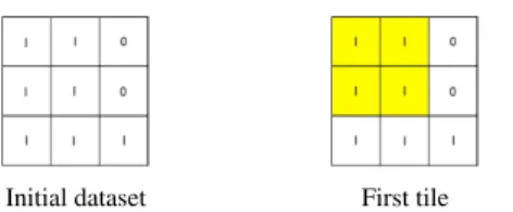
Data mining has contributed numerous techniques for finding patterns in (Boolean) matrices. One fundamental approach is that oftiling(Geerts et al, 2004). A tile is a rectangular area in a Boolean matrix represented by set of rows and columns such that all values on the corresponding rows and columns in the matrix are equal to 1.
One is typically not interested in any tile, but in maximal tiles, i.e., tiles that cannot be extended. For instance, Figure 1 shows a binary dataset and two tiles. The first tile consists of the first and second column together with the first and second row. All entries for these rows and columns are 1s. Furthermore, it cannot be expanded as adding the third column or row would also include 0 values. The second tile consists of all three columns and the third row. Together these two tiles “cover” the whole dataset, that is, all cells with value 1 in the matrix belong to one of the tiles. The area of a set of tiles, denoted asarea(T, D), is the number of cells (7 in our example) in the (union of the) tilesT occurring in the datasetD
Initial dataset First tile Second tile
Fig. 1:Example of Boolean tiles and their coverage
Definition 5 (Maximumk-Tiling)Given a binary datasetD and a positive integer k, find a tilingT consisting of at mostktiles and maximizingarea(T, D).
We now formalize tiling as a relational data factorization problem and then solve it using ASP. Rather than restricting ourselves to Boolean values as in the traditional formulation, we consider the relational case. The standard way of dealing with tables in attribute-value datasets was to expand them into a sparse Boolean matrix (with one Boolean for every value). In contrast, our formulation employs the attribute-value format directly.
Given a relation db(Value,Attr,Transct), denoting that transaction Transcthas
ValueforAttr, the task is to find a set of tiles that can be applied to the transactions to summarize the datasetdb. Here, a tile is a set of attribute-value pairs.
Fig. 2:Relational tiling: two relational tiles (right) in a toy dataset (left) concerning cars.
The two example tiles can be expressed as
tile(i1,fair,state).tile(i1,old,age).in(i1, t1).in(i1, t3).
tile(i2,gas,fuel).tile(i2,sport,type).in(i2, t1).in(i2, t2).
where the first argument of eachtileis the index of the tile, the second is the value of the attribute, and the third argument is the name of the attribute. When tileIis applied to a transactionT (i.e., it occurs in the transaction), this is denoted byin(I, T). We call a set of tiles atiling.
We would like to factorize the initial dataset, represented as a set of db(fair,
state, t1),db(old,age, t1),. . ., using the followingshapequery:
approx(Attr,Value,Transct)←tile(Indx,Value,Attr),in(Indx,Transct). (1)
To reason about the coverage of the shape, i.e., which transactions and attributes are covered in the dataset (indicated by color in Figure 2), we use the following definition:
covered(Transct,Attr)←approx(Attr,Value,Transct).
For instance,covered(t1,age)holds becausetile(i1,old,age)andin(i1, t1)hold. To specify the maximum k-tiling problem, we need the following constraints.
one-value-attribute: for every attribute of a tile there is at most one value:
←tile(Indx,Val1,Attr),tile(Indx,Val2,Attr),Val16=Val2. (2)
no-tile-intersection: tiles do not overlap in the same transaction
←in(I1, T),in(I2, T),tile(I1, V, A),tile(I2, V, A), I16=I2. (3)
no-overcoverage: tiles cannot “overcover” the transaction, that is, they are only
allowed to cover tuples that are in the dataset;
←tile(Indx,Value,Attr),in(Indx,Transct),not db(Value,Attr,Transct). (4)
number-of-patterns(K): there are at mostk-tiles (numbered from 1 tok):
Indx= 1∨Indx= 2∨. . .Indx=k←tile(Indx,Value,Attr).
Furthermore, the maximum k-tiling problem searches for the k tiles that maximize the area. This leads to an instance of thesimilarityscore defined by
coverage: #{(T, A) :covered(T, A)}. (5)
The statement above correspond to the standard mathematical function optimization notation, that reads as follows: count (#) the cardinality of the set ({·}) of tuples
(T, A)such that (:)covered(T, A)holds. When we translate this statements into ASP formulation we have to use special syntax of ASP (#maximize) to capture this math-ematical formulation.
Listing 4:Maximumk-Tiling ReDF Model
Input:datasetdband constantK
Shape:approx(Attr,Value,Transct)←tile(Indx,Value,Attr),in(Indx,Transct)
Find: the set of ground factstile(·),in(·)
Satisfying:no-tile-intersection∧no-overcoverage
∧number-of-patterns(K)∧one-value-attribute
Maximizing:coverage
To illustrate the advantages of our declarative and modular approach, let us consider a small variation of the tiling task, in which tiles may overlap.
Fig. 3:Example of a 0/1 database with a tiling consisting of two overlapping tiles
(darkest shaded area corresponds to the intersection of the two tiles), due to Geerts et al (2004)
Overlapping tiling Figure 3, taken from Geerts et al (2004), illustrates a Boolean dataset with two overlapping tiles. We investigate and present two new variations of maximumk-tiling: overlapping and noisy tiling. The first investigates the global pat-tern mining task, when the overall coverage is optimized, allowing overlaps between tiles. The second investigates the task when, ink-maximum tiling, a tile can have a number of mismatches as covering a transaction. It is straightforward to change the assumption in our ReDF framework (and the corresponding ASP implementation). For the first task, it only involves replacing the constraintno-tile-intersection
by the following constraint.
overlapping-tiles(N): two tiles in one transaction can intersect only on at
mostN attributes:
←in(I1, T),in(I2, T),tile(I1, V, A1),tile(I2, V, A2), I16=I2,#{A1=A2}> N.
To model the variation that tolerates some noise in the data, we can replace constraint
no-overcoverageby
noisy-overcoverage(N): every tileI can overcover at mostN attributes in
every transactionT where it occurs:
←tile(I, V, A),in(I, T),not db(V, A, T),#{A}>N.
4.2 The Discrete Basis Problem (DBP) and Boolean Matrix Factorization (BMF)
BMF has been extensively studied by Miettinen (2012), resulting in the well-known ASSO algorithm. Let us now show how it can be expressed as ReDF problem. As a starting point we take the same shape (Eq. 1) as in the tiling example in Subsec-tion 4.1. However, we need to change the constraints to reflect the different prop-erties of the desired solutions: tiles may now overlap, since one is not interested in tiles per se, but in good coverage of the dataset. That is why we remove the
no-tile-intersectionandno-overcoverageconstraints, and introduce
a notion of ‘overcoverage’ instead, by means of the following definition:
overcovered(T, A)←approx(V, A, T),not db(V, A, T).
In the Discrete Basis Problem, the scoring function maximizes the number of covered elements, while minimizing the overcovered ones. The latter term can be simply defined as:
overcoverage: #{(T, A) :overcovered(T, A)}.
We specify the high-level DBP model in Listing 5.
Listing 5:ReDF Model for the Discrete Basis Problem
Input:datasetdband constantsK, α
Shape:approx(Attr,Transct)←tile(Indx,Attr),in(Indx,Transct)
Find: the set of ground factstile(·),in(·)
Satisfying:number-of-patterns(K)
Maximizing:coverage−α×overcoverage
This formulation mimicsThe Discrete Basis Problem(Miettinen et al, 2008). That is, Kplays the role of the basis size andαmimics the bias towards rewarding covering and penalizing overcovering (the flags--bonus-coveredand
--penalty-overcoveredin ASSO).
It is well-known that tiling andBoolean matrix factorization(BMF) are closely related (Miettinen, 2012). Hence, let us also briefly show how BMF can be realized in our framework. It corresponds to an instance of DBP where only binary values (true and false) are possible and theno-overcoverageconstraint applies. Hence, it is required that the factorization undercovers the initial dataset, i.e., if there is a 0 in a position in the original dataset, then there cannot be a 1 in the approximation. Therefore, the optimization criterion of DBP is further simplified and we obtain the following BMF model, without overcovering, in Listing 6.
Listing 6:BMF without overcovering
Input:datasetdband constantK
Shape:approx(Attr,Transct)←tile(Indx,Attr),in(Indx,Transct)
Find: the set of ground factstile(·),in(·)
Satisfying:number-of-patterns(K)∧no-overcoverage
Column
Ro
w
20 40 60
40
30
20
10
(a)Regular Column
Ro
w
20 40 60 80
50
40
30
20
10
(b)With penalties Column
Ro
w
20 40 60 80
50
40
30
20
10
(c)With penalties and noise
Fig. 4:Re-arranging a matrix in block-diagonal form (Animals dataset): (a) regular, (b) with penalties,
(c) with noisy blocks and penalties
4.3 Discriminative k-pattern set mining
A common supervised data mining task is that of discriminative pattern set min-ing (Knobbe and Ho, 2006). Let db(Value,Attr,Transct) be a categorical dataset,
positive(T) (negative(T)) be the set of positive (negative) transactions, and k the number of tiles. Then, the task is to find extensions of the relationstile(Indx,Value,Attr) andin(Indx,Transct) such that positive and negative transactions are discriminated. A standard interpretation is to find tiles that cover as many positive and as few negative ones as possible (Liu et al, 1998). The only required change in the model concerns the scoring function (and assigning some weight to the errors):
#{T :covered(T),positive(T)} −α#{T :covered(T),negative(T)}, (6) whereαis a constant that represents the weights for the errors made. It is typically a domain specific parameter (the cost of covering a negative example by a rule, i.e., the false positive cost or a weight of a negative example). Let us denote the coverage of the positive transactions ascoverage+(left set term in Eq. 6) and the coverage of negative ascoverage−(right set term in Eq. 6).
Given that we have nono-overcoverageconstraint and negative transactions can be covered, the optimization criterion is given by
similarity(T) =coverage+−α×coverage−. This corresponds to the high-level model in Listing 7.
Listing 7:ReDF Discriminative Patter Set Mining Model
Input:datasetdband constantsK, α
Shape:approx(Attr,Value,Transct)←tile(Indx,Value,Attr),in(Indx,Transct)
Find: the set of ground factstile(·),in(·)
Satisfying:number-of-patterns(K)∧no-overcoverage∧one-value-attribute
Maximizing:coverage+−α×coverage−
4.4 Block-diagonal matrix form
block-diagonal structure of a matrix can be used to parallelize certain matrix com-putations. An illustration of block-diagonalization (several variants) of the Animals dataset is depicted in Figure 4.
We reduce it to a form of tiling. The shape query is the same as in tiling but the constraints are different: if a tileI1has an attributeA, then a tileI2cannot use the same attribute. A similar constraint is imposed on theinpredicate and transactions stating that each itemAcan belong to only one tile
item-blocking: ←tile(I1, A),tile(I2, A), I16=I2. Only one tile can occur in a transactionT.
transaction-blocking: ←in(I1, T),in(I2, T), I16=I2.
We also modify the optimization criterion to take into account elements not cov-ered by a tile but blocked by this tile. Every tile that selects attributes and transac-tions prohibits other tiles to use these attributes and transactransac-tions by means of the
item-blockingandtransaction-blocking constraints. We penalize
ex-cessive usage of attributes and transactions by a single tile. We do this to improve the block form of the matrix, since in this task we are not just interested in a tiling with maximal coverage, but in a tiling that maximizes the number of elements on the diagonal and minimizes the number of elements everywhere else. To enforce this we introduce two functions:
item-penalty: #{(T, A) :approx(T, A0), not covered(T, A)}
transt-penalty: #{(T, A) :approx(T0, A), not covered(T, A)}
Then, the whole problem is formulated in Listing 8.
Listing 8:ReDF Block-Diagonal Model
Input:datasetdband constantsN, α, β
Shape:approx(Attr,Value,Transct)←tile(Indx,Value,Attr),in(Indx,Transct)
Find: the set of ground factstile(·),in(·)
Satisfying:transaction-blocking∧item-blocking
one-value-attribute∧noisy-overcoverage(N)∧no-tile-intersection
Maximizing:coverage−α×transt-penalty−β×item-penalty
If we omititem-penaltyandtranst-penalty, we obtain the standard optimization function for tiling. In the experimental section we evaluate the effect of the presence of this penalty.
5 Beyond Classic Problems
Section 2 already provided thesellsexample for decomposing a ternary relation into three binary ones. In the shape for thesellsexample in Listing 3 there is no latent variable: there are only attributes from the original dataset. Since there is no latent variable, there is no “pattern” to be found for which the optimization criterion needs to be optimized, which allowed us to use a simple error function using only one type of atom.
However, latent variables can also be useful in a purely relational setting. Let us illustrate this on an example inspired by the ArXiv community analysis example of Gopalan and Blei (2013). Assume we are given a relationpublishedInwith attributes
Author,University, andVenue, specifying that an author belonging to a particular uni-versity publishes in a particular venue. Furthermore, assume we want to factorize this relation into the relationapprox (A,U,V) by introducing a latent attributeTopic, de-noted asT. The latent topic variable clusters authors, universities and venues together in such a way that their join results in publications.
We obtain the following high-level model in Listing 9, whereαis the constant that indicates the relative cost of overcovering an element and the integer constantk is the number of value that the latent variable (T) can take:
approx(A, U, V)←interestedIn(A,T),specializedIn(U,T),inField(V,T).
Listing 9:ReDF Purely Relational
Input:datasetdband constantsK, α
Shape:approx(A, U, V)←interestedIn(A,T),specializedIn(U,T),inField(V,T).
Find: the set of ground factsinterestedIn(·),specializedIn(·),inField(·)
Satisfying:number-of-patterns(K)
Maximize:coverage−α×overcoverage
The corresponding model without latent variables would be different only in the de-composition shape, i.e., it would look like
approx(A, U, V)←worksAt(A,U), publishesAt(A,V), knownAt(U,V).
Discriminative relational learning In the spirit of discriminative pattern mining, de-scribed in Subsection 4.3, we can also do discriminative learning in the purely rela-tional setting. To do so, we assume that the relation has an extra argument Co-Author and we would like to discriminate the dataset by a particular Co-Authorc+, i.e.,
coverage+(A, U, V)←approx(A, U, V),publishedIn(A, U, V, c+).
coverage−(A, U, V)←approx(A, U, V),publishedIn(A, U, V, C), C 6=c+. (7)
6 Implementation
This section describes how ReDF models can be implemented in ASP. We do this for the basic problem of tiling, as well as for the purely relational data factorization presented before. Implementations of the other variations are included in Appendix C. Our primary implementation is written in clasp, can be used with the clasp system (Gebser et al, 2012; Brewka et al, 2011) and will be made available online upon acceptance of this manuscript.
6.1 General computation methods: greedy and sampling approaches.
In all described problems, the goal is to findk patterns or tiles, where a pattern is interpreted as a set of facts corresponding to a particular value of the latent variable. We will follow an iterative approach to finding these patterns, in which the discovery of the next pattern or tile will be encoded in ASP. We will consider both agreedyand asamplingalgorithm for realizing this. The sampling approach is intended for better scalability and will be evaluated in Section 7.1.
Greedy model. The greedy approach is described in Algorithm 1. Essentially, when the next bestpatternhas been computed (wherepatternis a set of facts asso-ciated with thepatternidentifier, e.g., in tiling a pattern is a set of transactions and attributes), it is added to the current set ofpatterns. The specific part for each tile is represented byexecuteProgramand is encoded separately in ASP. Note that this greedy, iterative approach to findingkpatterns is very common in pattern mining. Theoretical bounds on the solution quality of the greedy approach have been stud-ied in the context of the maximumk-set coverage problem (Hochbaum and Pathria, 1998; Feige, 1996); more details can be found in Appendix F.
Algorithm 1:Greedy execution model
input :datais the dataset
output:patternsis the set of patterns
patterns← ∅;
fori∈[1, k]do
pattern←executeProgram(data,patterns, i);
patterns← {pattern} ∪patterns;
Column sampling execution model.To improve scalability, we employ a sampling approach. Interestingly, our approach is different from most existing sampling tech-niques in data mining: instead of sampling a rows or patterns, we sample columns. Algorithm 2 presents the column sampling approach we propose. The key difference with the greedy approach is that instead of determining the next best pattern on the
Algorithm 2:Column sampling execution model
input :datais the dataset
input :Nis the number of samples
input :αis the relative size of a sample
output:patternsis the set of patterns
patterns← ∅;
fori∈[1, k]do
maxPattern← ∅;
forj∈[1, N]do
sample←getColumnSample(data, α);
pattern←executeProgram(sample,patterns, i);
ifscore(pattern)>score(maxPattern)then
maxPattern←pattern;
patterns← {maxPattern} ∪patterns;
Listing 10:Greedy maximumk-tiling formalization in answer set programming
1 %one-value-attribute; it generates at most one value per attribute
2 0{tile(currentI, Value, Attribute) : valid(Attribute, Value)}1 :−col(Attribute). 3 %no-overcoverage
4 over covered(currentI,T) :−notdb(Value, Attribute, T), tile(currentI, Value, Attribute), transaction(T). 5 %no-tile-intersection
6 intersect(T) :−currentI != Index, tile(currentI, Value, Attribute), tile(Index, Value, Attribute), in(Index,T). 7 %defines presence of tiles in transactions
8 in(currentI,Transct) :−transaction(Transct),notover covered(currentI, Transct),notintersect(Transct). 9 %definescoveragefunction
10 covered(Transct, Attribute) :−in(Index,Transct), tile(Index, Value, Attribute). 11 #maximize[covered(Transct, Attribute)].
6.2 Data mining problems expressed in the framework
The maximumk-tiling problem can be encoded in answer set programming as in-dicated in Listing 10. The code implements the greedy model, i.e., Algorithm 1, for the maximumk-tiling problem with a fixed number of tiles (Geerts et al, 2004). It assumes we have already found an optimal tiling forn−1tiles, and indicates how to find then-th tile to cover the largest area. Then-th tile is calledcurrentIin the list-ing. Further, we have information about the names of the attributes and the possible values for each attribute through predicatescol(Attr)andvalid(Attr,Value). That is,
col(A)is an unary predicate that encodes possible column indices, andvalid(A, V)
Theorem 1 (Correctness of the greedy ASP tiling encoding) The ASP program P defined by the Listing 10 computes thek-th largest tile w.r.t. the scoring function
coverage(5) as extensions of the predicates tile(k,·,·)and in(k,·)in its answer setA, provided that the dataset is represented extensionally through the predicates db, valid, and col and the k−1 already found tiles are represented extensionally through the predicates tile(I,·,·)and in(I,·)forI∈[1, k−1].
For the proof, see Appendix B. The clasp encodings for the other models are sketched in Appendix C.
6.3 Purely relational data factorization
In Section 5 we presented a factorization of the publishedInrelation into three bi-nary relations. It constitutes a proof-of-concept prototype model in ASP and could be improved by, e.g., incorporating heuristics.
The general structure of the ASP encoding is similar to thesellsexample in List-ing 3: we indicate here only a possible optimization for the relation generators. We use the left-to-right order of the atoms in the schema (replicated below) while gener-ating candidates for the factorization.
Listing 11:Generators for the model without a latent variable into three binary relations
1 0{works at(A,U) }1 :−published in(A,U,V).
2 0{publishes at(A,V)}1 :−published in(A,U,V), works at(A,U).
3 0{known at(U,V) }1 :−published in(A,U,V), works at(A,U), publishes at(A,V).
Implementation differences.When we generalize the factorization encoding with two relations to three relations, we observe a slight implementation difference be-tween them. Factorization with the two relation shapes can be naturally implemented using the core ASP generate-and-test paradigm. Once we have guessed an extension for a certain value of the latent variable, we propagate it to the second relation and test against the constraints. This strategy is often deployed in specialized algorithms (Geerts et al, 2004; Miettinen et al, 2008). For a multiple relation shape we guess an extension of one relation, then we constrain the possible values we generate for the second value (e.g., see Line 2 in Listing 11). In general, we can search for one at a time using a greedy strategy (as in tiling). Theoretically, we can simultaneously search for values of a latent variable by replacing the fixed latent parameter by a vari-able and searching over the latent parameter as well. The work of Guns et al (2013b) provides evidence that this approach does not scale well, unless special propagators are introduced into the solver. This technique would allow extending the method to other shapes with more than three relations.
7 Experiments
a number of tasks compare the results and runtimes to those obtained by specialized algorithms. Since we here use generic problem formulations and generic solvers that have neither been designed nor optimized for the tasks under consideration, we can-not expect the approach to be as efficient as specialized algorithms. However, what is more important is that we demonstrate that all tasks formalized and prototyped using the ReDF framework can be solved using a unified approach.
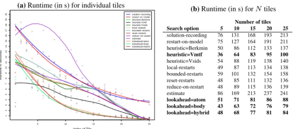
Experimental setup and datasets.The ASP engine we use is 64-bit clingo (clasp with the gringo grounder) version 3.0.5 with the parameter--heuristic=Vmtf
(see Appendix A for details on the parameters) and all experiments are executed on a 64-bit Ubuntu machine with Intel Core i5-3570 CPU @ 3.40GHz x 4 and 8GB memory, except for Maximumk-tiling on Chess and Mushrooms datasets where In-tel Xeon CPU with 128GB of memory (all single-threaded) has been used due to high memory requirements. For most experiments we use the datasets summarized in Ta-ble 1, which all but one originate from the UCI Machine Learning repository (Bache and Lichman, 2013). TheAnimals (with Attributes) dataset was taken from Osher-son et al (1991). For the purely relational factorization task, the data and experiment results are described separately in the corresponding subsection.
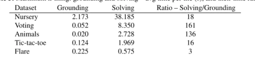
In Subsection 7.1 we show how ReDF formulations of existing data mining tasks (from Section 4) can be solved using the implementation presented in Section 6, afterwards in Subsection 7.2 we show the results of the purely relational data factor-ization task. The ASP solver parameters used in the experiments and a breakdown of individual solving steps and their runtimes determined by the meta-experiment are presented in Appendix A.
7.1 Solving existing tasks
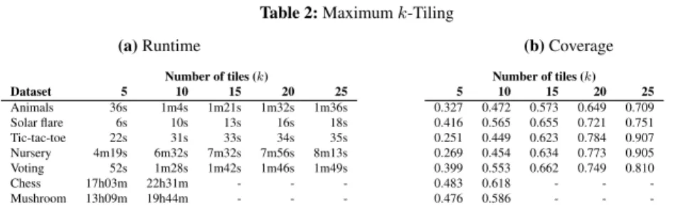
Maximum k-Tiling in Categorical Data We first consider the Maximum k-Tiling problem from Section 4.1 and present timing and coverage results in Table 2 obtained on all datasets from Table 1.
In all cases the problem specification given in Listing 10 was used to greedily minek = 25tiles. Since the problem becomes more constrained as the number of tiles increases, runtime decreases for each additional tile mined. We therefore report total runtime and coverage for different values ofk, i.e., for different total numbers of tiles. Onlyk= 10tiles were mined on Chess and Mushroom due to long runtimes.
Effect of sampling As we can see from Table 2a, runtimes are quite long on datasets like Mushroom. To address this issue, we use the sampling procedure of
Table 1:Dataset properties. For each dataset, we specify whether the attributes have Boolean or
categor-ical domains, the number of tuples and attributes, and the average number of distinct values per attribute
Dataset Attributes # tuples # attributes Avg # values per attribute
Animals Boolean 50 85 2
Solar flare categorical 1 389 11 3.3
Tic-tac-toe categorical 958 10 2.9
Nursery categorical 12 960 8 3.4
Voting categorical 435 17 3.0
Chess (Kr-vs-Kp) categorical 3 196 36 2.1
Table 2:Maximumk-Tiling
(a)Runtime
Number of tiles (k)
Dataset 5 10 15 20 25 Animals 36s 1m4s 1m21s 1m32s 1m36s Solar flare 6s 10s 13s 16s 18s Tic-tac-toe 22s 31s 33s 34s 35s Nursery 4m19s 6m32s 7m32s 7m56s 8m13s Voting 52s 1m28s 1m42s 1m46s 1m49s
Chess 17h03m 22h31m - -
-Mushroom 13h09m 19h44m - -
-(b)Coverage
Number of tiles (k) 5 10 15 20 25 0.327 0.472 0.573 0.649 0.709 0.416 0.565 0.655 0.721 0.751 0.251 0.449 0.623 0.784 0.907 0.269 0.454 0.634 0.773 0.905 0.399 0.553 0.662 0.749 0.810
0.483 0.618 - -
-0.476 0.586 - -
-Algorithm 2 with the following parameters:α = 0.4andN = 20, i.e., 40% of all attributes were selected uniformly at random for each sample and 20 samples were used. Intuitively, the larger the sample size and the more samples, the better we ap-proximate the exact result.
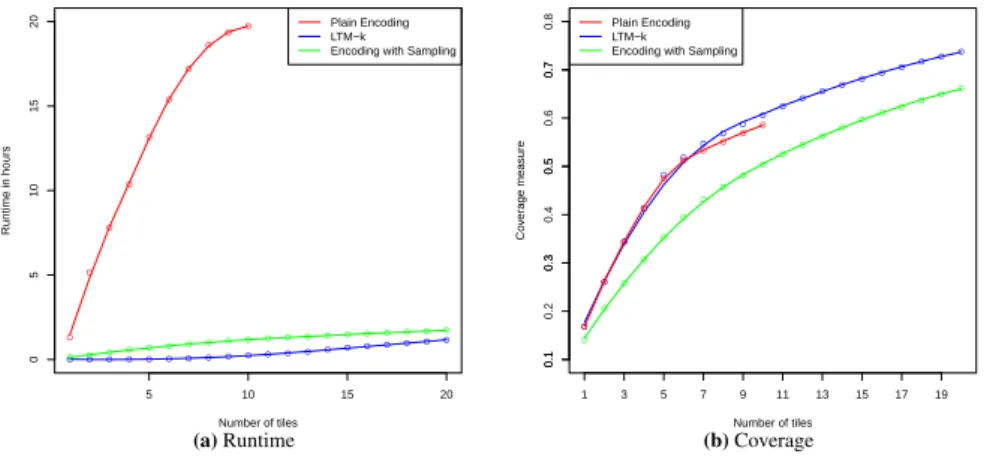
With the given parameters, we attain an order of magnitude improvement in run-time: instead of 19 hours with the regular algorithm, using sampling it takes only one hour to compute 10 tiles as indicated in Figure 5a. The effect of using sampling on coverage can be seen in Figure 5b: the first tiles that are mined have lower cov-erage than when sampling is not used, but after a while the difference in covcov-erage with LTM-k remains more or less constant and even slightly decreases. LTM-k is the original, specialized tiling algorithm, to which we compare next.
Comparison to a specialized algorithmWe now compare the performance of the ASP-based implementation of LTM-k greedy strategy to that of a specialized im-plementation2. Figures 5a and 5b present both runtime and coverage comparisons obtained on Mushroom, both for our approach (with and without sampling) and the specialized miner.
Without sampling, we can see that our approach gives the same results in terms of the coverage as the LTM-k algorithm. This is as expected though, since both LTM-k and our approach guarantee to find an optimal solution in each iteration. The slight difference between the two coverage curves in Figure 5b is caused by the fact that multiple tiles can have the same (maximum) area, and some choice between those has to be made. Although these choices are typically made deterministically, the differ-ent implemdiffer-entations make decisions based on differdiffer-ent criteria, resulting in slightly different tilings.
Unfortunately, the ASP solver is not as efficient as the specialized miner as can be seen in Figure 5a, and the generality of the approach comes at the cost of longer runtimes. However, as already discussed, using a sampling approach can substantially decrease the runtime. Experiments on other datasets showed similar behavior to that depicted here.
Overlapping tiling To evaluate the overlapping tiling task from Subsection 4.1, we apply the model in Listing 12 (ASP encoding in Appendix C) to the five smaller datasets from Table 1. We experiment with two levels of overlap, i.e., parameterNis set to either 1 or 2: tiles can intersect on at most one or two attribute(s). As the results
2
● ● ● ● ● ● ● ● ● ●
5 10 15 20
0
5
10
15
20
Number of tiles
Runtime in hours
Plain Encoding LTM−k Encoding with Sampling
● ● ● ● ● ● ● ● ● ● ● ● ● ● ● ● ● ● ● ● ● ● ● ● ● ● ● ● ● ● ● ● ● ● ● ● ● ● ● ● (a)Runtime ● ● ● ● ● ● ● ● ● ● ● ● ● ● ● ● ● ● ● ● 0.1 0.2 0.3 0.4 0.5 0.6 0.7 0.8
Number of tiles
Co v er age measure Plain Encoding LTM−k Encoding with Sampling
0.1
0.3
0.5
0.7
1 3 5 7 9 11 13 15 17 19
● ● ● ● ● ● ● ● ● ● ● ● ● ● ● ● ● ● ● ● ● ● ● ● ● ● ● ● ● ● (b)Coverage
Fig. 5:Tiling comparison (runtime, coverage) with LTM-k (Mushroom dataset)
Table 3:Maximumk-Tiling with overlap. The maximal allowed overlap is limited by parameterN
(a)Runtime
Number of tiles (k)
Dataset N 5 10 15 20 25 Animals 1 1m10s 2m28s 3m46s 4m24s 4m47 2 1m39s 4m10s 6m26s 7m40s 8m10s
Solar flare 1 8s 13s 17s 21s 24s
2 8s 15s 20s 25s 29s
Tic-tac-toe 1 24s 41s 49s 52s 53s
2 23s 43s 51s 55s 56s
Nursery 1 5m00s 8m19s 10m10s 10m48s 11m12s 2 5m43s 9m32s 11m9s 11m50s 12m12s Voting 1 1m10s 2m19s 2m53s 3m8s 3m15s 2 1m39s 3m34s 4m35s 5m9s 5m33s
(b)Coverage
Number of tiles (k) 5 10 15 20 25 0.327 0.475 0.583 0.663 0.722 0.332 0.482 0.592 0.675 0.742 0.433 0.595 0.684 0.734 0.756 0.452 0.602 0.685 0.731 0.755 0.253 0.451 0.626 0.781 0.898 0.253 0.451 0.626 0.781 0.898 0.268 0.454 0.633 0.772 0.905 0.268 0.454 0.633 0.772 0.905 0.403 0.558 0.675 0.765 0.828 0.409 0.571 0.683 0.762 0.819
in Table 3 show, allowing limited overlap can lead to a small increase in coverage, but runtimes also increase due to the costly aggregate operation in Line 1 of Listing 12.
However, what is important to emphasize here is that only a small change in the problem formalization is sufficient to allow for overlap in the tilings, while the solver can still solve the problem without any further changes. And although the runtimes are longer when more overlap is allowed, the difference with the basic, non-overlapping setting is moderate.
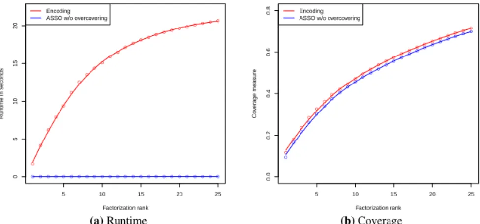
Boolean matrix factorization (BMF) We perform Boolean matrix factorization (Sec-tion 4.2) by applying the formaliza(Sec-tion of Listing 13 and compare the results to those obtained by ASSO3(Miettinen, 2012) with the no-overcoverage flag (-P1000). The factorization rankkis incremented by one in each iteration, and meanwhile coverage gain and runtime are measured. The results for Animals are presented in Figure 6 and show that coverage is almost identical to that obtained by ASSO. Again, this is unsurprising, as our implementation follows the same solving strategy. However, runtimes are several times higher, which is due to the usage of a general solver that is not optimized for this type of task. Results obtained on other datasets are very similar and are therefore not presented here.
3
● ● ● ● ● ● ● ● ● ● ● ●● ●● ●●● ●●●●●●●
5 10 15 20 25
0 5 10 15 20 Factorization rank
Runtime in seconds
●●●●●●●●●●●●●●●●●●●●●●●●● Encoding
ASSO w/o overcovering
(a)Runtime ● ● ● ● ● ● ● ● ● ●● ● ●● ●● ●● ●● ●● ●●●
5 10 15 20 25
0.0 0.2 0.4 0.6 0.8 Factorization rank Co v er age measure Encoding ASSO w/o overcovering
● ● ● ● ● ● ● ● ● ● ●● ●● ●● ●● ●● ●● ●● ● (b)Coverage
Fig. 6:Boolean matrix factorization on datasets Animals. Runtime and coverage are depicted for different
factorization ranks.
(a)Runtime (in s) to minek-th discriminative pattern on Chess dataset (α= 1, i.e., positive and negative tuples are weighted equally)
(b)Discriminative mining coverage on Chess and Tic-tac-toe datasets (α= 1, i.e., positive and negative tuples are weighted equally)
Tic-tac-toe (k= 5) Chess (k= 10) Covered− 92 (27.7%) 160 (7%) Covered+ 626 (100%) 864 (95.5%) Difference 534 704 Runtime 0.52s 18m48s
Fig. 7:Discriminative pattern set mining summary: runtime (left) and coverage (right)
Discriminative pattern set mining Here we demonstrate how the discriminative k-pattern mining model from Section 4.3 can be solved. For this we use Chess and Tic-tac-toe from Table 1, each of which has a binary class label indicating whether a game was won or not and can therefore be naturally used for this task.
● ● ● ● ● ● ● ●
1 2 3 4 5 6 7 8
0.70
0.75
0.80
0.85
0.90
0.95
1.00
Number of rules
Precision
● ●
● ●
● ● ● ●
α=5
α=1
(a)Precision
● ●
● ●
● ●
● ●
1 2 3 4 5 6 7 8
0.2
0.4
0.6
0.8
1.0
Number of rules
Recall
● ●
● ●
● ● ● ●
0.3
0.5
0.7
0.9
α=5
α=1
(b)Recall
Fig. 8:Discriminative pattern set mining (Tic-tac-toe dataset): precision (left) and recall (right) for
dif-ferentα, i.e., for varying weights of covering negative transactions
drops heavily. This confirms that the search space shrinks when the problem becomes more constrained, i.e., the number of answer sets decreases with the addition of more constraints.
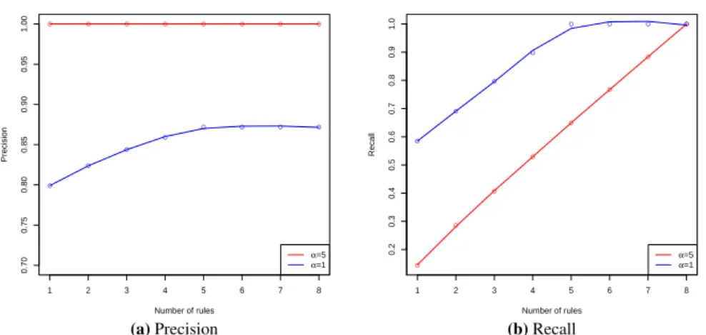
We next show the influence of the αparameter, i.e., the relative weight of cov-ering positive and negative tuples in the optimization criterion. By increasingα, the ‘penalty’ for covering a negative tuple is increased and the algorithm can be forced to select more conservative rules. We investigate the effect of this parameter by mea-suring and comparing precision and recall of the obtained pattern sets forα= 1and α= 5. Figure 8 shows that precision goes to1whenαis increased, while recall is decreased but this can be compensated by mining a larger number of patterns4.
This task differs from the previous one in its optimization criterion: positive cov-erage penalized by negative covcov-erage allows for fast inference and discovery of the optimal solution, which results in shorter runtimes than for tiling.
Matrix block-diagonal form We apply three versions of the encoding to the Animals dataset (Osherson et al, 1991). The results presented in Figure 4 demonstrate that the Animals dataset can be re-arranged into block-diagonal form using our proposed framework. The runtime in all experiments are on the order of seconds. Parameters used in the experiments wereα= 3
20andβ= 1
20. Figure 4c demonstrates the model from Section 4.4, with the same α,β andN = 1. The low-level encoding of this model is given in Listing 15.
7.2 Purely relational data factorization
In Section 5 we described how to model the factorization ofpublishedIn(Author, Uni-versity, Venue)into three binary relations with a latent variableTopic. We now eval-uate whether the standard ASP solver can solve this task. Unfortunately, we cannot
Fig. 9:Clustering in topics by ReDF. Red nodes represent co-authors, blue their university cities, white nodes venues and green topics that bind them together. If there is an edge between a topic and a node, then there is a corresponding element in the relation (i.e.,interestedIn,specializedInorinField)
expect a generic solver to handle enormous datasets such as the one from ArXiv as described by Gopalan and Blei (2013). Instead, we demonstrate a proof-of-concept of solving the model in Listing 16 on a moderate dataset.
We constructed a dataset for a well-known colleague from the data mining com-munity: Bart Goethals (Antwerp University). We collected his publication list from Microsoft Academic Search5and extracted for each paper the publication venue, and all co-authors together with their corresponding affiliations (i.e., the last known af-filiation for each author in this list of papers). Each unique combination of venue, co-author, and affiliation resulted in a tuple in thepublishedInrelation. The complete dataset contains 57 tuples over 19 universities, 38 authors, and 15 venues.
Intuitively, if a set ofauthorsfrom a set ofuniversitiespublish in a set ofvenues, then there must be an underlying researchtopicthat unites them. Hence, by factoriz-ing the relation into three separate relations, we cluster each of the entity types into a (fixed) number of topics, as indicated by the value of the latentTopicvariable.
The results for factorization using K = 12topics andα = 12 are presented in Figure 9, including co-authors (red), universities (blue), publication venues (purple),
and topics (green). To determine the number of topicsK, we tracked the optimization criterion while increasingKand stopped when this no longer improved.
Since the task is of an exploratory character, we can only qualitatively evaluate the results. We observe that all data mining venues are located together in the center, connected to the same topics. SEBD, an Italian database conference, stands apart, and there is also a separate block for database and computing venues DaWaK and SAC. Manual inspection of the results indicates the topics (or clusters) to be coherent and meaningful: they represent different affiliations and groups of co-authors that Bart Goethals has collaborated with. For example, topic5contains the SDM conference, the University of Helsinki, and three co-authors specialized in Data Mining. Hence, this topic could be described as “Data mining collaboration with the University of Helsinki”, which makes perfect sense as Bart Goethals was previously a researcher in Helsinki.
Not all authors are represented in the factorization. How much of thepublishedIn
dataset is covered depends on the number of topicsK(which was chosen as described before). The higher the cardinality of the pattern set, the larger the total coverage. Thecoveredelements positively contribute to coverage, whereas theovercovered el-ements contribute negatively. This implies that each pattern is chosen such that the number ofcoveredandovercoveredelements are balanced and the optimization cri-terion is maximized. In general, covering all authors with few patterns would lead to significant overcovering of the original dataset, while introducing too many patterns would create clusters with only one author (which is clearly undesirable, since these clusters would not be meaningful).
The decompositions, as the one depicted in Figure 9, could serve as a basis for new analyses. For example, we might visualize the intersection of common (latent) topics shared by two researchers. We outline possible examples in Appendix E.
Relational factorization without a latent variable. In Section 5, we also described a factorization that does not use any latent variables (analog to thesellsexample in Listing 3 from the introduction section). We evaluate this model using Listing 11 on the same dataset as used in the previous experiment, i.e., the co-author relation
publishedIn(Author, Uni, Venue)for Bart Goethals.
In general, factorizations do not perfectly match the original relation (i.e.,error6= 0), but in this particular case the system found a lossless solution. It is easy to see that this will not always be possible though. For instance, let us assume we keep multiple affiliations per author in the dataset. For example, apart from a fact
p(bonchi,barcelona,pakdd), there may be another factp(bonchi, pisa, pakdd)in pub-lishedIn. Although the same factorization would be found by the solver, the found solution would be imperfect as the latter fact is not represented in the factorized rela-tion.
Solving this task was computationally easy, since there is no latent variable to iterate over: the runtime was only0.01s. Table 4 presents a summary.
Table 4:Experimental summary for pure relational factorizations from Subsection 5
With a latent variable #Transactions58 Overall runtime14s Avg runtime1.1s #Topics12 Avg atoms per topic5.4
Without a latent variable #Transactions Overall runtime Correct #Incorrect Avg factor size
58 0.01s 58 0 45
researchers in the field of data mining: Jiawei Han and Philip S. Yu. In this example all publications belonging to either researcher are considered a class. Since DBLP data does not have authors affiliations, we replace this attribute with the publication date converted to a categorical variableM ∈ {old,recent,new}, using the following rule: if the date is later than 2010, it is represented as “new”; if it is between 2005 and 2010, then it is “recent”; otherwise it is “old”. The complete dataset contains around 6000 ground atoms of the following form:paper(Author,Age,Venue,Han\Yu). The goal is to predict whether the paper is co-authored by Han or Yu based on author, venue and age using discriminative rules as defined in Eq. 7. In this experiment the shape is
approx(A, M, V)←author(A, T),paperAge(M, T),venue(V, M),
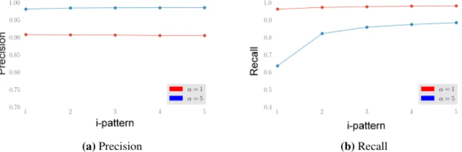
whereT is a latent variable. As for the previous discriminative experiment, in Figure 10 we present an overview of the dependency of precision and recall on the number of patterns andα, the penalty for covering the incorrect class. Runtimes are similar as in Figure 7a. ASP finds an optimal solution in half an hour and then spends a substantial amount of time to prove it is indeed the best solution. We therefore used a time limit of one hour per pattern speedup the computation. This limit was only reached in the computation of the first pattern, for both values ofα.
In Figure 10 we see that, depending on the number of patterns and penalty for covering the wrong class (α), we can obtain a classifier with different precision and recall6.
(a)Precision (b)Recall
Fig. 10:Discriminative learning in the purely relational setting; precision (left) and recall (right) for
differentα, i.e., for two weights of covering negative atoms.
7.3 Runtime discussion
In this section we have seen a number of experiments that solve ReDF problems using generic solving technology, i.e., answer set programming. As we can see in Figures
5a and 6, specialized algorithms are substantially faster than ASP. On datasets of moderate size, however, generic solvers obtain reasonable runtimes, as indicated by the results in Tables 2a, 3a, and 7b, and Figures 6 and 7a. For the purely relational data factorization task from Section 5 we present a summary of the experiments in Table 4. In these experiments, computation time ranged from several seconds to few minutes.
8 Related Work
Our work is related to 1) previous work on generalizing problem definitions and solutions in factorization, 2) existing forms of relational decomposition, and 3) ap-proaches in inductive and abductive logic programming, and 4) the use of declarative languages and solvers for data mining.
8.1 General models for pattern mining
Our work can be related to a number of approaches that have generalized some of the tasks addressed in Section 5. Lu et al (2008) used BMF as a basis for defining sev-eral data mining tasks and modeled them using integer linear programming. While Lu et al (2008) also used a general purpose solver, it is restricted to Boolean matrix products involving only two Boolean matrices. In a similar manner Li (2005) defined aGeneral Model for Clustering Binary Data, using matrix factorization to model several well-known clustering methods. The framework supports only one possible factorization shape, a lower-level modeling language, and requires complete parti-tions as well as specialized algorithms for different problems. In our approach, the shape of the factorization is separated from the constraints and optimization criterion. Biskup et al (2004); Fan et al (2012) investigated inverse querying and the prob-lem of solving relational equationse1(D) = e2(D)exactly under several assump-tions, that could be used to compute exact solutions to a restricted form of ReDF. However, this approach does not seem to allow for approximations and the use of loss functions.
8.2 Decomposition of databases, tensors, and real-valued matrices
ReDF is related to several forms ofrelational decomposition, a term that has been heavily overloaded in the literature. Hence, it is imperative that we present an overview and contrast existing paradigms to our own work. Moreover, ReDF is also related to decomposition methods for real-valued matrices.
never based on the data (extension), but only on the schema (intension); 3) decompo-sition is always lossless, i.e., factorization is always exact for any possible extension, and never an approximation. An interesting exception isRelational Decomposition via Partial Relations(Berzal et al, 2002), where one is looking for partially satisfied dependencies in the data and then uses these partial dependencies to derive a normal form. It does take into account data, but only to mine additional schema constraints in the decomposition.
Relational decomposition in tensor calculus.Kim and Candan (2011) extend clas-sical tensor factorization, CP decomposition, to deal with datasets composed of sev-eral relations, i.e., CP is gensev-eralized to multi-relational datasets. This requires adding relational algebra operations to CP. Key differences are: the data consists of several tables, with a schema to join them at the end; the shape is always the same and a tensor is decomposed into a sum of terms having the same structure; the optimization function is fixed; no user constraints are supported.
Decomposition of real-valued matrices. Let us start with SVD (Singular Value Decomposition) (Golub and Van Loan, 1996), the best-known method in this area, which gives an optimal rank-kdecomposition of a real-valued matrixAinto a com-position of three matricesU ΣVT, whereU andV are orthogonal real-valued matri-ces andΣ is a diagonal non-negative matrix with singular values ofA. One of the key problems with SVD in the context of relational and Boolean factorization is that U andV may contain negative values, which make interpretation in the relational setting problematic. To overcome this issue NNMF (Non-Negative Matrix Factoriza-tion) has been introduced (Paatero and Tapper, 1994). Still, there are two key issues with the usage of NNMF and SVD for relational and Boolean data.
First of all, for a Boolean matrixAthere is no clear relation between its real value rank, denoted rankR(A), and its Boolean rank, denoted rankB(A), (rankR≥0(A) de-notes the non-negative rank). We know that the following inequalities hold (Mietti-nen, 2009):
rankR(A)≤rankR≥0(A)
rankB(A)≤rankR≥0(A) (8)
Furthermore, there are examples where rankR(A) = n and rankB(A) = log(n) (where A isn×n matrix) (Miettinen, 2009), which implies that there are cases where Boolean factorization could be preferable over real-valued matrix factoriza-tion, i.e., there are cases where we can obtain a smaller decomposition if we use dis-crete rather than real-valued methods. Also, if we look at approximate ranks (when the approximation is set within), Equation 8 above does not hold, i.e., there is no clear connection between NNMF and Boolean ranks in the approximate case.
Finally, as ReDF is defined over discrete values in the presence of the hard con-straints, all the problems described above (rank inequalities, optimization over reals, uninterpretable values, etc) apply to the comparison of ReDF with real-valued matrix factorizations as well.
8.3 Relational learning
ReDF is also related to some well known techniques in inductive logic programming and statistical relational learning and even to abductive reasoning.
Several frameworks forabductionhave been introduced over the years (Denecker and Kakas, 2002; Flach and Kakas, 2000). In abduction, the goal is to find a (minimal) hypothesis in the form of a set of ground facts that explains an observation. Abductive reasoning uses a rich background theory as well as integrity constraints; it also uses a set of clauses defining the predicate in the observation. The differences with ReDF are that ReDF uses a much simpler shape definition and no real background theory. On the other hand, abductive reasoning proceeds in a purely logical manner, and typically does neither take into account multiple facts in the observation nor does it use complex optimization functions. There also exist similarities between ReDF and fuzzy abduction (Vojt´as, 1999; Miyata et al, 1995), but we differ in the core assumptions we make: all rules and constraints in our setting are deterministic, as well as the evidence that needs to be derived. Also, ReDF has the shape constraint, which allows to derive only specific explanations in a form of a factorization.
Meta-interpretive learning (Muggleton et al, 2015) uses templates together with a kind of abductive reasoning to find a set of rules and facts in a typical inductive logic programming setting. While it can use much richer templates and background theory, it uses neither constraints nor optimisation functions like ReDF does.
Kok and Domingos (2007) introduced a probabilistic framework based on Markov logic together with the EM principle to realize statistical predicate invention. This captures what the authors callmultiple relational clusteringand addresses essentially the same task as theinfinite relational modelof Kemp et al (2006). Statistical predi-cate invention shares several ideas with our approach: it employs a kind of query or schema to denote the kind of factorization one wants and also imposes some hard constraints on the possible solutions. On the other hand, its optimization criterion is built-in and based on the maximum likelihood principle, the framework seems re-stricted to a kind of block modeling approach, essentially clustering the different rows and columns into different blocks, and the approach is inherently probabilistic.
8.4 Declarative data mining
of integer linear programming is quite popular in data mining and machine learning; e.g., Chang et al (2008). While the choice of a particular framework for modeling and solving may lead to both different models and performances, it should be possible to use alternative frameworks, such as constraint programming or integer programming, for modeling and solving ReDF problems.
Aftrati et al (2012) extended the typical structure of the mining problem using three-level graphs that represent a chain of relations in the multi-relational setting: authors writing papers, and papers being about certain topics. The goal is to find the subgraphs that satisfy particular constraints and optimization criteria. E.g., an author is an authority if the number of topics he has written papers on is maximal. They pro-vide various interesting discovery tasks and solve them using integer programming.
9 Conclusions
The key contribution of this paper is the introduction of the framework of relational data factorization, which was shown to be relevant for modeling, prototyping, and experimentation purposes.
On the modeling side, we have formulated several well-known data mining tasks in terms of ReDF, which allowed us to identify commonalities and differences be-tween these data mining tasks. One advantage of the framework is that small changes in the problem definition typically lead to small changes in the model. Furthermore, ReDF allowed us to model new types of relational data mining problems.
We have not only modeled problems, but also demonstrated that these models can be easily translated into concrete executable ASP encodings. The experiments have shown the feasibility of the approach, especially for prototyping, and especially with the sampling technique. The runtimes were typically not comparable with highly op-timized and much more specific implementations that are typically used in data min-ing. Still they could be run on reasonable datasets of modest size (e.g., Mushroom and Chess have approximately185 000and115 000non-empty elements respectively).
Directions for future research include investigating the use of alternative solvers (such as constraint or integer programming), the study of heuristics and local search, and the expansion of the range of tasks to which ReDF can be applied. For example, a general ReDF framework is needed to factorize evidence for probabilistic lifted in-ference, where the shape of the factorization crucially affects the overall performance of the algorithm (Van den Broeck and Darwiche, 2013).
Acknowledgments.We would like to thank Marc Denecker, Tias Guns, Benjamin Negrevergne, Siegfried Nijssen, and Behrouz Babaki for their help and assistance, and last but not least the ICON project (FP7-ICT-2011-C) and FWO for funding this work.
References