MacMullin_unc_0153D_15737.pdf

(1)

VALIDATION OF THE BACKGROUND MODEL FOR THE M_AJORANA DEMONSTRATOR

Jacqueline MacMullin

A dissertation submitted to the faculty of the University of North Carolina at Chapel Hill in partial fulfillment of the requirements for the degree of Doctor of Philosophy in

the Department of Physics and Astronomy.

Chapel Hill 2015

(2)

c

○ 2015

(3)

ABSTRACT

Jacqueline MacMullin: Validation of the Background Model for the Majorana Demonstrator.

(Under the direction of John Wilkerson.)

The observation of neutrinoless double-beta decay would confirm the Majorana na-ture of the neutrino and would allow one to potentially determine the mass of neutrinos. The goal of the Majoranacollaboration is to develop a tonne-scale Ge-76-based neu-trinoless double-beta decay experiment. Currently, efforts are underway to construct the Majorana Demonstrator, a 44.8-kg array of germanium crystals, located at the 48500 level of the Sanford Underground Research Facility (SURF) in Lead, SD. The goal of the Demonstrator is to demonstrate the ability to construct a detector composed of an array of germanium crystals while maintaining an unprecedented low background that is essential for the observation of neutrinoless double-beta decay.

Before the assembly and operation of the Demonstrator, a single test cryostat was built. This cryostat, referred to as the Prototype Cryostat, was built to test the clean assembly procedures that are to be used for the Demonstrator. Understanding the backgrounds of the Majorana Demonstratoris of the upmost importance and for this reason, much effort has been put into creating an accurate background model. While achieving the lowest possible background is the goal of the D_emonstrator, this is not necessarily true of the Prototype Cryostat, whose main purpose is to improve on cryostat assembly procedures, analysis routines and the like. Nevertheless, understand-ing the backgrounds of the Prototype Cryostat can help to verify the background model of the Demonstrator. Thus a background model of the Prototype Cryostat has been developed using the same techniques that are being used to develop the background

(4)

(5)

To Mom and Dad. Thank you for your endless love and support.

(6)

TABLE OF CONTENTS

LIST OF FIGURES . . . xiii

LIST OF TABLES . . . xxi

LIST OF ABBREVIATIONS . . . xxv

1 INTRODUCTION . . . 1

1.1 Neutrino Oscillation and Mass . . . 1

1.1.1 Neutrinoless Double-Beta Decay . . . 3

1.2 The MajoranaDemonstrator . . . 6

1.2.1 Low-Mass Design and Shielding . . . 11

1.2.2 Assay and Material Preparation . . . 15

1.2.3 Detector Technology . . . 17

1.3 Prototype Cryostat . . . 19

2 DATA ACQUISITION, PROCESSING AND SELECTION . . . 25

2.1 Overview . . . 25

2.1.1 Detector Readout and Data Acquisition . . . 25

2.1.2 Data Processing . . . 27

2.1.3 The GRETINA Digitizer Cards . . . 27

2.2 Data Selection . . . 28

(7)

2.2.2 Bad Timestamp . . . 34

2.2.3 High Rate . . . 35

2.2.4 Digitizer Board and/or Channel Outage . . . 36

2.2.5 Change in Detector Gain . . . 39

2.2.6 Shift in Onboard Energy Determination . . . 44

2.2.7 Incorrect Onboard Energy Assignment . . . 45

3 GAMMA-PEAK CHARACTERIZATION . . . 54

3.1 An Introduction to the Peak-Fitting Function . . . 54

3.2 Minimization Techniques and Parameter Errors . . . 58

3.3 Single Peak-Fitting Function Parameter Correlations . . . 61

3.4 Multiple Peak-Fitting Function . . . 63

3.4.1 Parameter Correlations . . . 65

3.5 Conclusions and Future Work . . . 66

4 GAMMA-PEAK CHARACTERIZATION FOR THE DETECTORS OF THE PROTOTYPE CRYOSTAT . . . 71

4.1 Multi-Peak Fitting Routine . . . 71

4.1.1 Fitting Algorithm I . . . 72

4.1.2 Fitting Algorithm II . . . 73

4.1.3 Fitting Algorithm III . . . 74

4.2 Results . . . 75

4.3 Peak Shape Issues . . . 79

4.3.1 Double Peaking in S1D4 of the PC . . . 80

4.4 Future Work . . . 80

(8)

5 PROTOTYPE CRYOSTAT BACKGROUND MODEL . . . 85

5.1 Introduction . . . 85

5.2 MaGe: The Majorana and GerdaSimulation Toolkit . . . 86

5.3 Modeling the Prototype Cryostat Geometry . . . 87

5.3.1 Inaccuracies in the PC Geometry . . . 93

5.4 Component Grouping in the Prototype Cryostat Background Model . . 97

5.5 Energy Resolution for MC-Generated Energy Spectra . . . 102

5.6 Inaccuracies in the PC Background Model . . . 103

5.6.1 The Decay of Protactinium-234m in Geant4 . . . 103

5.6.2 Excluding the Upper Uranium-238 Decay Chain from Simulations 108 5.6.3 Disequilibrium in the Uranium-238 and Thorium-232 Decay Chains110 5.6.4 Excluding Alphas from Simulations . . . 112

5.6.5 Other Possible Sources of Background . . . 114

6 COMPARING THE PROTOTYPE CRYOSTAT BACKGROUND MODEL TO DATA . . . 116

6.1 Introduction . . . 116

6.2 Low-Background Data Used . . . 116

6.3 Component Grouping for the Monte Carlo Fit to Data . . . 117

6.3.1 The Effective Number of Events Simulated for a Group . . . 122

6.4 Simultaneous Multi-Detector Fit . . . 124

6.4.1 Minimization Function . . . 127

6.5 Low-Background Data Fit Results . . . 129

6.6 A Systematics Test . . . 139

(9)

6.7 Discussion of Results and Future Work . . . 147

7 CONCLUSIONS . . . 163

A RELEVANT CALCULATIONS . . . 165

A.1 For the case of Fitting a Single Peak . . . 165

A.1.1 Peak Centroid . . . 165

A.1.2 Peak Variance . . . 166

A.1.3 Uncertainty of Peak Centroid . . . 168

A.1.4 Uncertainty of Peak Variance . . . 169

A.2 For the case of Fitting Muliple Peaks . . . 169

A.2.1 Uncertainty of Peak Centroid . . . 169

A.2.2 Uncertainty of Peak Variance . . . 171

A.2.3 Uncertainty of Sigma . . . 173

A.2.4 Uncertainty of Tau . . . 174

A.2.5 Uncertainty of Htail . . . 174

A.3 Estimation of the Contribution from Missing Components in the PC Background Model . . . 174

A.3.1 Gasket . . . 174

A.3.2 Outer Copper Shield . . . 175

A.3.3 Cables . . . 176

A.4 Technique Used to Simulate Radioactivity in a Group of Components in MaGe . . . 177

B DETECTOR PEAK SHAPE CHARACTERIZATION . . . 181

B.1 S1D2 of the PC (Detector B8717) . . . 183

(10)

B.1.1 Summary of Fit Results . . . 183

B.1.2 Individual Peak Fits . . . 194

B.2 S1D3 of the PC (Detector Ponama II) . . . 200

C MAGE MASSES AND MATERIALS OF PROTOTYPE CRYOSTAT COMPONENTS . . . 272

C.1 Overview . . . 272

C.2 Detector Masses . . . 276

C.3 String 1 Copper Components: OFHC versus EFCu . . . 277

C.4 String 2 Copper Components: OFHC versus EFCu . . . 279

(11)

D MONTE CARLO FIT RESULTS . . . 283

D.1 MC-Generated Energy Spectra . . . 283

D.2 Low-Background Data with 83 Fit Parameters . . . 292

D.2.1 S1D2 of the PC (Detector B8717) . . . 292

D.2.2 S1D3 of the PC (Detector Ponama II) . . . 295

D.2.7 Histogram of Pulls . . . 310

D.3 High-Radon Data with 1 Fit Parameter . . . 312

D.3.7 Histogram of Pulls . . . 324

D.4 High-Radon Data with 83 Fit Parameters . . . 327

(12)

D.4.6 S3D5 of the PC (Detector B8473) . . . 342 D.4.7 Histogram of Pulls . . . 345

(13)

LIST OF FIGURES

1.1 The Sensitivity of a Tonne-Scale 76Ge 0νββ Experiment . . . 7

1.2 The Uranium-238 Decay Chain . . . 8

1.3 The Thorium-232 Decay Chain . . . 9

1.4 The Detector Unit of the M_ajorana D_emonstrator . . . 12

1.5 A Detector Unit of the Majorana Demonstrator . . . 13

1.6 The String Design for the Majorana Demonstrator . . . 13

1.7 A String of the M_ajorana D_emonstrator . . . 14

1.8 The Compact Shield Design for the MajoranaDemonstrator . . . 16

1.9 The Three Strings of the PC . . . 21

2.1 An overview of the PC DAQ system. . . 26

2.2 Overview of Background and Calibration Data Taken with the Prototype Cryostat . . . 30

2.3 Digitizer Rates for a Subset of Background Data. . . 38

2.4 Pulser Centroid for a Subset of Background Data. . . 42

2.5 Detector Rates for a Subset of Background Data. . . 43

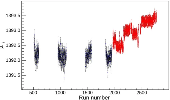
2.6 Pulser Centroid for S1D4 for a Subset of Background Data. . . 44

2.7 Onboard versus Offline Energy for a Subset of the Background Data for S3D5. 46 2.8 Onboard versus Offline Energy for All of the Background Data for S3D5. . 47

2.9 Onboard versus Offline Energy for a 228_{Th Calibration Run for S3D5. . . .} ₄₉

2.10 Linear Fit to Figure 2.9. . . 49

2.11 Linear Fit to Figure 2.9 with the±5-sigma Band. . . 50

2.12 Data from Fig. 2.9 with Omissions. . . 50

(14)

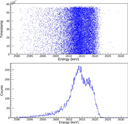
2.13 Energy Spectrum of Calibration Events Cut from Data Selection in

Sec-tion 2.2.7. . . 52

2.14 Energy Spectrum of Background Events Cut from Data Selection in Sec-tion 2.2.7. . . 53

3.1 Example of a Fit to a Single Gamma Peak. . . 59

3.2 Sigma Contours for µ and Hstep, Htail, σ and τ . . . 64

3.3 Sigma Contours for Select Parameters of the Multi-Peak Fitting Function . 68 4.1 Result from Fitting S3D2 During a Calibration Run Using the Multi-Peak Fitting Routine . . . 76

4.2 Parameter σ0 for S3D2 for Five Calibration Runs . . . 77

4.3 S1D4’s Peak Shape Behavior Over a Broad Range of Energy. . . 81

4.4 Timestamps of the Events in One of S1D4’s Double Peaks. . . 82

4.5 Parameters bτ for S1D3 . . . 83

4.6 Parameters mτ for S1D3 . . . 84

5.1 The PC String Arrays as Modeled in M_aG_e . . . 90

5.2 The PC Thermal Shield as Modeled in MaGe . . . 91

5.3 The PC Cryostat Lids as Modeled in MaGe . . . 92

5.4 The Uranium-238 Decay Chain . . . 105

5.5 Gamma Peaks in MC-Generated Energy Spectrum from the Decay of 234Pa 106 5.6 Histogram of TrackIDs for 234_{Pa and} 214_{Bi Gamma Peaks . . . .} ₁₁₀

5.7 CDF of TrackID Histograms for 234_{Pa and} 214_{Bi . . . .} ₁₁₁

(15)

6.1 A Toy Drawing Demonstrating the Need for Detector-Dependent Parameters 125 6.2 Count Rates from the Components of the MC-Fit to the Low-Background

Data . . . 135

6.3 The Best Fit to the Low-Background Data for S3D2 . . . 136

6.4 The Best Fit to the Low-Background Data for S3D2 and the Pull . . . 138

6.5 Histogram of the Pull from the MC-Fit to the Low-Background Data for S3D2139 6.6 Count Rates from the Components of the MC-Fit to the Low-Background Data for S3D2 . . . 140

6.7 Measured 222_{Rn Inside the Shielding of the PC over Three Days . . . .} ₁₄₁

6.8 Count Rates from the Components of the 83-Parameter MC-Fit to the High-Rn Data . . . 148

6.9 Location of the Temperature Sensor Assemblies in MaGe. . . 154

B.1 Parameters σi for S1D2 . . . 184

B.2 Parameters bτ and mτ for S1D2 . . . 185

B.3 Parameters bH and mH for S1D2 . . . 186

B.4 The Centroid of Peak#1 for S1D2 . . . 188

B.9 Fits and Residuals for the Five Gamma Peaks of S1D2 in Calibration Data Set A . . . 195

B.10 Fits and Residuals for the Five Gamma Peaks of S1D2 in Calibration Data Set B . . . 196

B.11 Fits and Residuals for the Five Gamma Peaks of S1D2 in Calibration Data Set C . . . 197

(16)

B.12 Fits and Residuals for the Five Gamma Peaks of S1D2 in Calibration Data

Set D . . . 198

B.13 Fits and Residuals for the Five Gamma Peaks of S1D2 in Calibration Data Set E . . . 199

B.25 Fits and Residuals for the Five Gamma Peaks of S1D3 in Calibration Data Set D . . . 214

(17)

B.32 Fits and Residuals for the Five Gamma Peaks of S3D1 in Calibration Data

Set A . . . 225

(18)

B.66 Fits and Residuals for the Four Gamma Peaks of S3D5 in Calibration Data Set B . . . 268

(19)

D.1 Normalized MC-Generated Energy Spectra for S3D2 (1 of 8) . . . 284

D.9 The Best Fit to the Low-Background Data for S1D2 (1 of 2) . . . 293

D.21 Histograms of the Pulls from the Fit to the Low-Background Data for the Detectors in String One . . . 310

D.22 Histograms of the Pulls from the Fit to the Low-Background Data for the Detectors in String Three . . . 311

D.23 The Best 1-Parameter Fit to the High-Rn Data for S1D2 . . . 313

(20)

D.29 Histograms of the Pulls from the 1-Parameter Fit to the High-Rn Data for the Detectors in String One . . . 325

D.30 Histograms of the Pulls from the 1-Parameter Fit to the High-Rn Data for the Detectors in String Three . . . 326

D.31 The Best 83-Parameter Fit to the High-Rn Data for S1D2 (1 of 2) . . . 328

D.43 Histograms of the Pulls from the 83-Parameter Fit to the High-Rn Data for the Detectors in String One . . . 345

(21)

LIST OF TABLES

1.1 The Half-Life of 2νββ and 0νββ in76Ge, 136Xe and 130Te. . . 5

1.2 Assay Values for Materials in the D_emonstrator . . . 18

1.3 Measured Detector Masses of the PC . . . 20

2.1 Number of Calibration Runs Before and After Data Selection Cuts . . . . 32

2.2 Percentage of Calibration Runs Cut from Each Data Selection Cut . . . . 32

2.3 Number of Background Runs Before and After Data Selection Cuts . . . . 33

2.4 Percentage of Background Runs Cut from Each Data Selection Cut . . . . 33

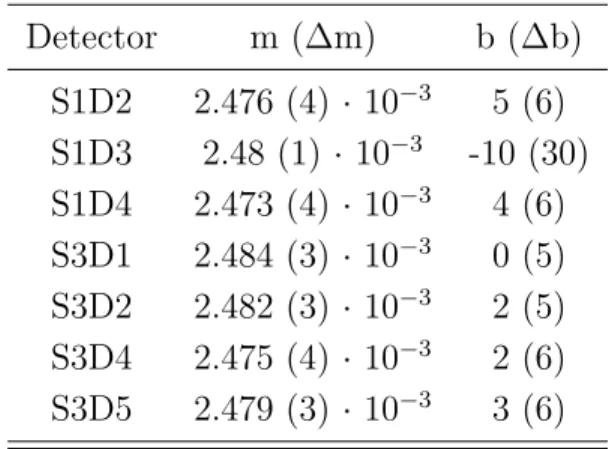
2.5 Results from Linear Fit to Onboard versus Offline Energy. . . 51

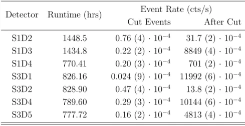
2.6 Performance of Event Cut in Section 2.2.7 on Calibration Data. . . 51

2.7 Performance of Event Cut in Section 2.2.7 on Background Data. . . 52

3.1 Best Fit Parameters from the Fit in Figure 3.1 . . . 58

3.2 Parameters in the Single Gamma-Ray Peak Simulations . . . 62

3.3 Parameters in the Multiple Gamma-Ray Peak Simulations . . . 67

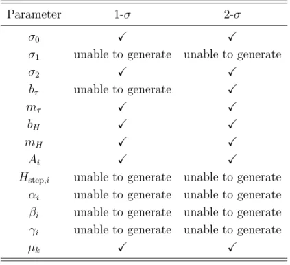
3.4 Status of Sigma Contours in the Multi-Peak Fitting Function . . . 67

4.1 Five Gamma Peaks Used in Multi-Peak Fitting Routine . . . 72

4.2 The Common Parameters Describing Each Detector’s Energy Response Func-tion . . . 77

4.3 Status of Multi-Peak Fitting Routine for All Calibration Data. . . 79

5.1 Groups Used in the PC Background Model Simulations . . . 99

5.2 Identified Gamma Peaks in Figure 5.5 . . . 107

5.3 Gamma Peaks from the Decay of 234Pa and 234mPa between 0.92 and 1.02 MeV . . . 107

(22)

6.1 Runtime of Low-Background Data Set for Each Detector . . . 117 6.2 Groups Used for Fitting the MC-Generated Energy Spectra to Data . . . . 120 6.3 Activities from MC Fit to Low-Background Data (1 of 3) . . . 131 6.4 Activities from MC Fit to Low-Background Data (2 of 3) . . . 132 6.5 Activities from MC Fit to Low-Background Data (3 of 3) . . . 133 6.6 Count Rate of the Low-Background Data and its MC Fit . . . 134 6.7 Activities from MC Fit to High-Rn Data (1 of 3) . . . 144 6.8 Activities from MC Fit to High-Rn Data (2 of 3) . . . 145 6.9 Activities from MC Fit to High-Rn Data (3 of 3) . . . 146 6.10 Count Rate of the High-Rn Data and its MC Fit . . . 147 6.11 Non-Zero, Detector-Independent Activities from MC Fit . . . 155 6.12 Non-Zero, Detector-Dependent Activities from MC Fit (1 of 2) . . . 156 6.13 Non-Zero, Detector-Dependent Activities from MC Fit (1 of 2) . . . 157

(23)

B.11 Peak #3 Parameters of S1D3 for All Calibration Data . . . 206 B.12 Peak #4 Parameters of S1D3 for All Calibration Data . . . 207 B.13 Peak #5 Parameters of S1D3 for All Calibration Data . . . 208 B.14 Peak Areas for S1D3 . . . 209 B.15 Common Parameters of S3D1 for All Calibration Data . . . 217 B.16 Peak #1 Parameters of S3D1 for All Calibration Data . . . 218 B.17 Peak #2 Parameters of S3D1 for All Calibration Data . . . 219 B.18 Peak #3 Parameters of S3D1 for All Calibration Data . . . 220 B.19 Peak #4 Parameters of S3D1 for All Calibration Data . . . 221 B.20 Peak #5 Parameters of S3D1 for All Calibration Data . . . 222 B.21 Peak Areas for S3D1 . . . 223 B.22 Common Parameters of S3D2 for All Calibration Data . . . 229 B.23 Peak #1 Parameters of S3D2 for All Calibration Data . . . 233 B.24 Peak #2 Parameters of S3D2 for All Calibration Data . . . 234 B.25 Peak #3 Parameters of S3D2 for All Calibration Data . . . 235 B.26 Peak #4 Parameters of S3D2 for All Calibration Data . . . 236 B.27 Peak #5 Parameters of S3D2 for All Calibration Data . . . 237 B.28 Peak Areas for S3D2 . . . 238 B.29 Common Parameters of S3D4 for All Calibration Data . . . 245 B.30 Peak #1 Parameters of S3D4 for All Calibration Data . . . 247 B.31 Peak #2 Parameters of S3D4 for All Calibration Data . . . 248 B.32 Peak #3 Parameters of S3D4 for All Calibration Data . . . 249 B.33 Peak #4 Parameters of S3D4 for All Calibration Data . . . 250 B.34 Peak #5 Parameters of S3D4 for All Calibration Data . . . 251

(24)

B.35 Peak Areas for S3D4 . . . 252 B.36 Common Parameters of S3D5 for All Calibration Data . . . 259 B.37 Peak #1 Parameters of S3D5 for All Calibration Data . . . 261 B.38 Peak #2 Parameters of S3D5 for All Calibration Data . . . 262 B.39 Peak #3 Parameters of S3D5 for All Calibration Data . . . 263 B.40 Peak #4 Parameters of S3D5 for All Calibration Data . . . 264 B.41 Peak #5 Parameters of S3D5 for All Calibration Data . . . 265 B.42 Peak Areas for S3D5 . . . 266

C.1 MaGe Masses and Materials of Prototype Cryostat Components: Cryostat and Surrounding Environment . . . 273 C.2 MaGe Masses and Materials of Prototype Cryostat Components: String

Arrays . . . 274 C.3 MaGe Masses and Materials of Prototype Cryostat Components: Detector

Mounts . . . 275 C.4 M_aG_e Masses and Materials of Prototype Cryostat Components:

(25)

LIST OF ABBREVIATIONS

0νββ neutrinoless double-beta decay 2νββ two-neutrino double-beta decay BEGe Broad Energy Germanium

CDF Cumulative Distribution Function

CP charge-parity

DAQ data acquistion

DQ data quality

GAT Germanium Analysis Toolkit GDMS Glow Discharge Mass Spectroscopy HPGe High-Purity Germanium

ICPMS Inductively-Coupled Plasma Mass Spectrometry JSON JavaScript Object Notation

KS test Kolmogorov-Smirnov test

KURF Kimballton Underground Research Facility LMFE Low Mass Front End

LNGS Laboratori Nazionali del Gran Sasso

MALBEK MajoranaLow-background BEGe at KURF

MC Monte Carlo

NAA Neutron Activation Analysis

NERSC National Energy Research Scientific Computing Center NLL Negative Log-Likelihood

NME Nuclear Matrix Elements

OFHC Oxygen-Free High thermal Conductivity

ORCA Object-oriented Real-time Control and Acquisition

PC Prototype Cryostat

PDF Probability Distribution Function

(26)

PDSF Parallel Distributed Systems Facility PEEK Polyether Ether Ketone

PMNS Pontecorvo-Maki-Nakagawa-Sakata P-PC p-type point contact

PSA pulse-shape analysis PTDB Parts Tracking Database PTFE Polytetrafluoroethylene

QRPA Quasiparticle Random Phase Approximation ROI region of interest

SBC Single Board Computer

SS Stainless Steel

STC String Test Cryostat

(27)

CHAPTER 1: INTRODUCTION

1.1 Neutrino Oscillation and Mass

In 1930 Pauli first proposed the existence of the neutrino to explain the continuous -rather than delta - energy distribution of the beta decay spectrum. Pauli proposed that the neutrino is a neutral particle that only interacts weakly. In 1956 the neutrino was first detected by Cowan and Reines [CC56]. In the following 60 years much progress has been made in understanding the properties of the neutrino. It is now known that there are three flavors of neutrinos – electron, muon and tau – with each flavor constituting a unique eigenstate. Furthermore there are three mass eigenstates and they can be written as a superposition of the flavor eigenstates and vice versa. The mixing of the flavor and mass eigenstates is described by Eq. 1.1, where the mixing matrix (with elements Uf i) is the Pontecorvo-Maki-Nakagawa-Sakata (PMNS) matrix

in Eq. 1.2 [Aal04, Ell02, LC08].

      νe νµ ντ       =      

Ue1 Ue2 Ue3

Uµ1 Uµ2 Uµ3

Uτ1 Uτ2 Uτ3             ν1 ν2 ν3       (1.1) U =      

c12c13 s12c13 s13e−iδ

−s12c23−c12s23s13eiδ c12c23−s12s23s13eiδ s23c13

s12s23−c12c23s13eiδ −c12s23−s12c23s13eiδ c23c13            

eiα1/2

0 0

0 eiα2/2 ₀

0 0 1

(28)

angles. Because the flavor and mass eigenstates are not the same, neutrinos oscillate between the three flavors as they propagate through space; hence the term “mixing”. The probability that a f-flavored neutrino will oscillate to a f0-flavored neutrino is given by Eq. 1.3 [Aal04].

P(νf →νf0₆₌_f) =

X i

Uf ie−i m2_{i L}

2E U∗ f0_i

2

P(νf →νf0₆₌_f) = sin22θsin2

1.27∆m2_ji

eV2

L(km)

Eν(GeV)

(1.3)

It can be seen from Eq. 1.3 that neutrino oscillation requires that neutrinos have a non-zero mass. Furthermore neutrino oscillation experiments are limited in that they can only determine the differences in the squares of the neutrino masses (i.e. ∆m2

ji;

Eq. 1.4).

∆m2_ji =m2_j −m2_i (1.4)

To measure the absolute differences in neutrino masses (∆m2

ji) and the mixing

angles (θij), neutrino oscillation experiments must optimize the distance between the

detector and the source of neutrinos (i.e. L of Eq. 1.3) relative to the energy of the neutrinos from the source (i.e. Eν of Eq. 1.3). Based on observations of solar neutrino

oscillations, it is known that ∆m2

21 > 0, however it is unknown if ∆m232 is positive

or negative. The unknown sign of ∆m2

32 presents two possible neutrino hierarchies: a

normal mass hierarchy if ∆m2

32 is positive and an inverted mass hierarchy if ∆m232 is

negative. The current values of ∆m2

32 and ∆m221 are in Eq. 1.5. Equation 1.6 gives the

current values of the neutrino mixing angles [Oli14].

(29)

however it is unknown if ∆m2

32 is positive or negative. The unknown sign of ∆m232

presents two possible neutrino hierarchies: a normal mass hierarchy if ∆m2₃₂ is positive and an inverted mass hierarchy if ∆m2₃₂ is negative. The current values of ∆m2₃₂ and ∆m2₂₁ are in Eq. 1.5 [Oli14]. Equation 1.6 gives the current values of the neutrino mixing angles.

∆m2₂₁= (7.53±0.18)·10−5eV2

∆m2₃₂=



  

  

(2.44±0.06)·10−3eV2 Normal Hierarchy (2.52±0.07)·10−3eV2 Inverted Hierarchy

(1.5)

sin2(θ12) =0.846±0.021 sin2(θ13) = (9.3±0.8)·10−2

sin2(θ23) = 

  

  

0.999+0−0..001018 Normal Hierarchy

1.000+0−0..000017 Inverted Hierarchy

(1.6)

The remaining three variables in the PMNS matrix (Eq. 1.2) are the phase factors:

α1, α2 and δ. If neutrino oscillation violates charge-parity (CP) symmetry the phase

factorδis non-zero. Given that the neutrino is a neutrally-charged particle, it is possible that the neutrino and anti-neutrino are the same particle that simply have a different chirality. If the neutrino is a Majorana particle (i.e. it is the same as its anti-particle), the phase factors α1 and α2 are required to fully describe the system.

1.1.1 Neutrinoless Double-Beta Decay

For some even-even nuclei, beta decay is energetically forbidden or strongly sup-pressed. It has been observed that these nuclei undergo two-neutrino double-beta

(30)

decay (2νββ) (Eq. 1.7).

(A, Z)→(A, Z+ 2) + 2e−+ 2 ¯νe (1.7)

If the neutrino is a Majorana particle, it is possible for such nuclei to decay via neutrinoless double-beta decay (0νββ) (Eq. 1.8).

(A, Z)→(A, Z + 2) + 2e− (1.8)

While 2νββ has been observed, 0νββ has not yet been observed. The observa-tion of this decay mode would confirm the Majorana nature of the neutrino [Sch82]. Furthermore, the observation of 0νββ would allow one to determine the mass of neutri-nos. Assuming light neutrino exchange moderates the neutrinoless double-beta decay process, the half-life is

h T10_/νββ2

i−1

=G0ν|M0ν|2m2ββ (1.9)

whereG0ν is the phase-space factor andM0ν is the Nuclear Matrix Elements (NME).

The effective Majorana mass, mββ, is expressed in Eq. 1.10 where mi are the mass

eigenstates andUei are the elements of the PMNS matrix (Eq. 1.2) that describe how

the electron flavor mixes with the neutrino masses.

mββ =

X

i

U_ei2 mi

(1.10)

(31)

Table 1.1: The half-life of 2νββ and 0νββ in76_Ge, 136_{Xe and} 130_Te.

Nuclide T12_/ν2 [10

21 _yr] _T0ν

1_/2 [10

25 _yr] 76_Ge ₁_.₈₄+0.14

−0.10 [Col13] >3.0 (90% C.L.) [Mac14] >1.9 (90% C.L.) [KK01]

136_Xe ₂_.₁₆₅_±₀_.₀₁₆

stat±0.059sys [Alb14] >1.9 (90% C.L.) [Gan13] >1.6 (90% C.L.) [Aug12]

130_Te ₀_.₇_±₀_.₀₉

stat±0.11sys [Arn11] ≥0.3 (90% C.L.) [Arn08]

disagree with one another up to a factor of two or three [Ber12]. Therefore it is impor-tant that if 0νββ is discovered it should be verified with another nuclide. This is true not only because of the uncertainty of the NME but also because of the rare nature of 0νββ. Even the most stringent upper limits on the half-life of 0νββ are no less than 1025 years, as seen in Table 1.1. There are about a dozen even-even nuclides that are candidates for 0νββ; the three nuclides listed in Table 1.1 were chosen because, to date, they place the best upper limit on the half-life of 0νββ. The best limit for130_Te

has been placed by the CUORICINO experiment [Arn08]. The best limit for136_{Xe has}

been placed by both the EXO-200 and KamLAND-Zen experiments [Aug12, Gan13]. And currently the best limit for 76_{Ge has been placed by the Heidelberg-Moscow and}

GERDA experiments [KK01, Mac14].

The nuclide76Ge is particularly interesting since, being a semiconductor, germanium has the advantage that it can serve as both the detector and source of 0νββ. The signature of 0νββ in 76_{Ge is a mono-energetic peak at 2039 keV; the endpoint of the}

2νββ continuous beta spectrum. Several experiments, past and present, are searching for 0νββ in 76_{Ge. While Table 1.1 states an upper limit on the half-life of 0}_νββ _in 76_{Ge, there has been a controversial claim of discovery. This claim was made by a}

subset of the Heidelberg-Moscow collaboration. Located at the Laboratori Nazionali

(32)

del Gran Sasso (LNGS) in Italy, the collaboration operated 11 kg of detectors enriched in76Ge and collected 71.7 kg-years of data. The collaboration did not claim discovery and put an upper limit on the half-life, as seen in Table 1.1. Later, a subset of the collaboration made a claim of discovery of 0νββ of 76Ge with a half-life of 1.19+2−0..9950·

1025 _{yrs [KK06, KK04]. As seen in Table 1.1, recent 0}_νββ _{experiments disagree with}

this claimed observation. This is particularly true of the GERDA experiment, which recently placed an upper limit (with the same nuclide,76_{Ge) at 3}_.₀_·₁₀25 _years.

1.2 The Majorana Demonstrator

Presently the Majorana collaboration is preparing to search for 0νββ in 76Ge. In order to fully probe the inverted hierarchy, a tonne-scale 76Ge 0νββ experiment is needed. The ultimate goal of the Majorana collaboration is to create a tonne-scale 76_{Ge 0}_νββ _{experiment that can probe the inverted hierarchy mass region with}

background rates not exceeding 1 cnts/ROI/ton/yr. (Where the region of interest (ROI) is 2037-2041 keV.)

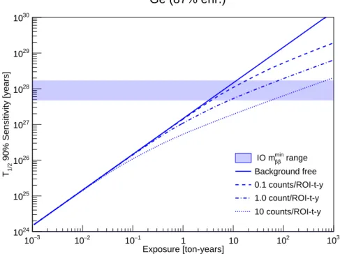
Figure 1.1 shows a tonne-scale Ge experiment’s sensitivity to 0νββ as a function of exposure and the background rate. From Fig. 1.1 it can be seen that with a background rate less than 3 cnts/ROI/ton/yr the Klapdor-Kleingrothaus claim can be fully tested after 0.03 tonne-years of exposure. Furthermore, with a background rate less than 1 cnts/ROI/ton/yr it would take roughly 10 tonne-years of exposure to fully probe the inverted hierarchy assuming the most optimistic NME.

This is an unprecedented low background for such an experiment and therefore great care is being taken to ensure such a background goal can be obtained. To achieve such a low background one must design an experiment that not only focuses on background reduction but background rejection. Backgrounds can generally be classified into two types: depth-dependent and depth-independent backgrounds.

(33)

Exposure [ton-years]

3 −

10 10−2 10−1 1 10 102 103

90% Sensitivity [years]

1/2

T

24

10

25

10

26

10

27

10

28

10

29

10

30

10

range min

β β IO m

Background free

0.1 counts/ROI-t-y

1.0 count/ROI-t-y

10 counts/ROI-t-y

Ge (87% enr.)

76

Figure 1.1: A tonne-scale 76_{Ge 0}_νββ _{experiment’s sensitivity as a function of exposure}

and the background rate. With a background rate less than 3 cnts/ROI/ton/yr the Klapdor-Kleingrothaus claim can be fully tested after 0.03 tonne-years of exposure. With a background rate less than 1 cnts/ROI/ton/yr it would take roughly 10 tonne-years of exposure to fully probe the inverted hierarchy [Det15].

(34)

Table of Contents Page -3-!decay !decay !decay !decay !decay 99.980%!decay

99.9%!decay

0.021%!decay

1.96x10 %-9 _!decay

0.020% - decay"

99.979% - decay" "- decay

"- decay

"- decay "- decay

"- decay

0.1% - decay" "-decay

!decay

"-decay 99.84%"-decay 0.16% IT decay

99.999 946%!decay 0.000 054% SF

1.7x10 % SF-9

Th 234 (24.10 day) Pa 234m (1.17 min.) Pa 234 (6.7 hr.) Th 230

(7.4x10 yr.)4

Ra 226 (1600 yr.) Rn 222 (3.8 day) Po 218 (3.1 min.) Po 218 (3.1 min.) Pb 214 (26 min.) Bi 214 (19 min.) Tl 210 (1.3 min.) Hg 206 (8.15 min.) Tl 206 (4.199 min.) Pb 206 (stable) Pb 210 (22 yr.) At 218 (1.5 sec.) Rn 218 (35 msec.) Po 214

(164 sec.)#

Bi 210 (5.0 day) Po 210 (138 day) U 238

(4.468x10 yr.)9

U

234

(2.4x10 yr.)5

Ne

24

(5.6x10-11%)

C

14

(3.2x10 %)-9

238_{U Decay Chain}

Figure 1.2: The 238U decay chain. Figure taken from [INL].

the detector or from surrounding materials; namely backgrounds from the decay of

238_U,232_{Th and} 40_{K. The radioactive nuclide} 40_{K predominantly (89%) beta-decays to}

the stable nuclide40_{Ca with the emission of a 1.3-MeV gamma. About 10% of the time}

it electron-captures to 40Ar with the emission of a 1.46-MeV gamma. The radioactive nuclides 238U and 232Th prove particularly troublesome since their daughter nuclides are not stable and therefore each nuclide has an associated decay chain, as pictured in Figs. 1.2 and 1.3. Considering the expected endpoint energy of the 0νββ, the main concern from the 232_{Th decay chain is the beta-decay of} 208_{Tl with the emission of a}

2.64-MeV gamma, and the main concern from the 238_{U decay chain is the beta-decay}

(35)

Table of Contents Page

-5-!-decay

!-decay

64.06%!-decay

!-decay

"decay

35.94%"decay

"decay

!-decay

Th

232

(1.405 x 1010yr.)

Ra 228 (5.75 yr.) Ac 228 (6.15 hr.) Tl 208 (3.053 min.) Ra 224 (3.66 day) Rn 220 (55.6 sec.) Po 216 (0.145 sec.) Pb 212 (10.64 hr.) Bi 212 (60.55 min.) Pb 208 (stable) Th 228 (1.9116 yr.) Po 212

(0.299µsec.)

232_{Th Decay Chain}

Figure 1.3: The 232_{Th decay chain. Figure taken from [INL].}

(36)

Another concern is 222_{Rn which is part of the} 238_{U decay chain. This nuclide is}

also present in the air. If present, 222Rn (or its daughter nuclides) can plate-out on exposed surfaces and then alpha decay. If any parts that have a direct line-of-sight to the detectors – or if the detectors themselves – are exposed to 222Rn, any emitted high-energy alphas could pose a threat to the ROI.

Depth-dependent backgrounds, as the name implies, reduces as the depth of the experiment’s location increases. This includes through-going and stopping muons and muon-induced fast neutrons [Mei06]. Also of concern are cosmogenically-induced back-grounds, such as the production of60Co in copper and 68Ge in the germanium crystals. Regardless of the depth, additional shielding is needed to reduce the backgrounds from natural radioactivity in the surrounding environment. In designing a tonne-scale exper-iment, one of the biggest questions is whether to use an active liquid shield or whether to use a passive compact shield. To help answer this question the Majorana and Gerda collaborations are working together to design a tonne-scale experiment while also operating differing – and yet complementary – experiments. The Majorana col-laboration is employing a compact shield design, while the Gerda collaboration is operating detectors inside of a liquid argon shield [Mac14]. By designing and operating complementary experiments, the Majorana and Gerdacollaborators are are able to combine their experiences to optimally design a tonne-scale experiment.

The M_ajoranacollaboration is building the M_ajoranaD_emonstrator: an ar-ray of High-Purity Germanium (HPGe) detectors inside of a compact shield located at the 48500level at Sanford Underground Research Facility (SURF). The Demonstrator consists of 44.8 kg of p-type point contact (P-PC) detectors with 29.7 kg enriched to 87%

76_{Ge and the remaining detectors fabricated from natural germanium (7.8%}76_{Ge). The}

(37)

also able to test the Klapdor-Kleingrothaus claim and search for physics beyond the Standard Model (e.g. light Weakly-Interacting Massive Particles (WIMPs) and ax-ions) [Fin13]. The Demonstrator will also play an important role in verifying sim-ulations of expected depth-dependent backgrounds. Previous studies have shown dis-agreement between muon-induced neutron production rates between different Monte Carlo (MC) codes. These neutrons do not pose a threat to the backgrounds of the Demonstrator but could pose a threat to a tonne-scale experiment. Therefore it is crucial that the Demonstrator help verify the muon-induced production rate by comparing simulations to data. Additionally, these simulations will help to verify the experiment’s overburden and rock composition that will be crucial to the success of a tonne-scale experiment if it is to be placed at the SURF facilities.

1.2.1 Low-Mass Design and Shielding

To reduce backgrounds the detectors of the Demonstrator are housed in low-mass assembly strings. Figures 1.4 and 1.6 are renderings of the low-low-mass detector unit and string respectively; Figs. 1.5 and 1.7 are photographs of a detector unit and string respectively. Nearly all the components of the detector and string parts are made from electroformed copper (shown in Figures 1.4 and 1.6 as the reddish-brown parts). This electroformed copper is grown at SURF, at the same depth as the location of the D_emonstratorand is referred to as Underground Electroformed Copper (UGEFCu). Any parts in the detector and string designs that are not made from UGEFCu are made from NXT-85. The Polytetrafluoroethylene (PTFE) NXT-85 is a Teflonr_manufactured

by DuPont and specially made in a clean-room environment.

The strings are arranged in arrays and positioned so to provide as much self-shielding as possible, while also giving shielding preference to the enriched detectors. The string arrays are attached to a coldplate and housed in vacuum-sealed cryostats. The

(38)

(39)

Figure 1.5: A photograph of a detector unit in the M_ajoranaD_emonstrator. Note, the detector unit is upside-down relative to Fig. 1.4.

Figure 1.6: The string design for the Majorana Demonstrator. Also included is the naming convention used for each part in the string.

(40)

(41)

Demonstrator will contain a total of two vacuum-sealed cryostats, with each cryo-stat mounted to its own vacuum system. Each cryocryo-stat also has its own thermosyphon and liquid nitrogen dewar. The dewars and vacuum systems for the cryostats sit out-side of the compact shield. Even at a depth of 48500, cosmogenic activity can be a concern and therefore additional shielding and vetoing capabilities are needed. The compact shield also provides the detectors protection from natural radioactivity in the surrounding environment (e.g. rock walls, concrete floor and lab furniture). Starting from the innermost cavity, the shielding consists of an inner layer of UGEFCu, an outer layer of Oxygen-Free High thermal Conductivity (OFHC) Cu, lead, an active muon veto, polyethylene and borated polyethylene. The cryostats, copper shields and lead shield are all enclosed in an air-tight Stainless Steel (SS) box that is purged with N2 gas that has been scrubbed free of 222Rn. The thermospyhon and all other copper

components that sit inside the inner Cu shield are made from UGEFCu. Figure 1.8 is a cross-sectional rendering of the two cryostats of the Demonstratorsituated inside the shielding. Each cryostat has its own thermosyphon, dewar and vacuum system but only one (of the two) is shown in the cross-sectional view. Further details on the vacuum, cryogenics and 222Rn-purge systems can be found in Ref. [Abg14].

1.2.2 Assay and Material Preparation

Nearly all the components inside the cryostats, the cryostats themselves and the innermost layer of the shielding are made form UGEFCu. That the experiment is built almost entirely from UGEFCu is a trait unique to the Majorana Demonstrator and should significantly contribute to the success of the Demonstratorachieving an ultra-low background. By electroforming its copper at the 48500 level of SURF, the Majoranacollaboration has been able to grow copper with low natural radioactivity and low cosmogenically-induced radioactivity. Furthermore the collaboration has been able to tightly control the machining process and surface exposure of the copper. After

(42)

Figure 1.8: A cross-sectional view of the compact shield design for the Majorana Demonstrator. The polyethylene and muon veto panels are colored purple for vi-sualization purposes. Each cryostat has its own vacuum system, thermosyphon and dewar but only one (of the two) is shown in the cross-sectional view.

(43)

air but also from possible 222_{Rn plate-out.}

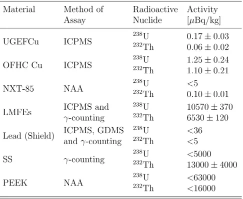
While most of the Demonstratorsupport structures and cryostats are made from UGEFCu there are other materials as well. All materials in the cryostat components and shielding have been carefully selected and then prepared for an ultra-clean envi-ronment. The M_ajoranacollaboration has conducted an extensive assay program to ensure all the materials used for the Demonstrator are of sufficient purity. Every material used in the Demonstratorhas been assayed by at least one of the following methods: gamma-ray spectroscopy, Neutron Activation Analysis (NAA) or mass spec-troscopy (in particular, Glow Discharge Mass Specspec-troscopy (GDMS) and Inductively-Coupled Plasma Mass Spectrometry (ICPMS)). Furthermore, just as the UGEFCu is handled in a cleanroom environment and cleaned with ultra-pure chemicals, so are all the materials in the D_emonstrator. Reference [Abgon] details each material that has been assayed by the Majorana collaboration, the method used, and the mate-rial’s radiopurity. Table 1.2 is a selected list of some of the materials, namely those that are present in the Demonstratorand the Prototype Cryostat (PC) (section 1.3) and frequently referenced throughout this thesis.

1.2.3 Detector Technology

To summarize thus far, the Majorana Demonstrator has been designed to reduce backgrounds by as much as possible using the following techniques.

• The Demonstrator is located deep underground to limit cosmogenic back-grounds.

• A majority of the Demonstrator parts are made from UGEFCu; the copper is grown underground to limit cosmogenically-induced backgrounds.

• The cryostats are surrounded by several layers of passive and active shielding to remove cosmogenic backgrounds and to reduce backgrounds from natural activity

(44)

Table 1.2: A selected list of materials used in the Demonstrator and PC and their assay values. For a complete list and further details see Ref [Abgon].

Material Method of Radioactive Activity

Assay Nuclide [µBq/kg]

UGEFCu ICPMS

238_U ₀_.₁₇_±₀_.₀₃ 232_Th ₀_.₀₆_±₀_.₀₂

OFHC Cu ICPMS

238_U ₁_.₂₅_±₀_.₂₄ 232_Th ₁_.₁₀_±₀_.₂₁

NXT-85 NAA

238_U _<₅

232_Th ₀_.₁₀_±₀_.₀₁

LMFEs ICPMS and

238_U ₁₀₅₇₀_±₃₇₀ γ-counting 232Th 6530±120 Lead (Shield) ICPMS, GDMS

238_U _<₃₆

and γ-counting 232Th <5

SS γ-counting

238_U _<₅₀₀₀

232_Th ₁₃₀₀₀_±₄₀₀₀

PEEK NAA

238_U _<₆₃₀₀₀ 232_Th _<₁₆₀₀₀

in the surrounding environment.

• Through an extensive assay campaign it has been confirmed that the bulk of the materials (used in the Demonstrator) are low in natural radioactivity. Fur-thermore every part is subjected to a through cleaning with ultra-pure chemicals to ensure little-to-no surface contamination.

• Following their manufacture, the detectors are never exposed to air and great efforts are made to ensure the string parts have limited air exposure; doing so limits the possibility of222_{Rn plate-out on surfaces.}

• A low-mass string design is used to hold the detectors.

(45)

cuts are being implemented on the detectors of the Demonstrator: a pulse-shape analysis (PSA) cut and a granularity cut. The Majoranacollaboration utilizes P-PC HPGe detectors. In a traditional coaxial detector the electrode is a well that extends from the bottom face of the cylindrical crystal, along the z-axis. On the other hand a P-PC detector has a point-like, shallow contact giving an extended range of drift times – the time it takes an electron-hole to drift to the point-contact. This allows one to better distinguish single-site events from multi-site events through PSA. A 0νββ

event would be a single-site event whereas many backgrounds (such as a gamma-ray interactions) are multi-site events. Thus the backgrounds of the Demonstrator can be further reduced by implementing a PSA cut. An additional benefit of using P-PC HPGe detectors is that they have a low intrinsic capacity, giving them great energy resolution.

The detectors of the Demonstrator are contained in strings and in turn, the strings are mounted to a coldplate in arrays. While the string-array configuration provides additional shielding to the inner-most detectors it also allows for an additional analysis cut: a granularity cut. Given that a 0νββ is an internal event in a detector, a granularity cut can be made to veto events that scatter in multiple detectors within a pre-determined time window. The granularity cut will reduce backgrounds from external gammas as well as cosmogenic backgrounds.

1.3 Prototype Cryostat

Before the assembly and operation of the Demonstrator, a single test cryostat was built. This cryostat, referred to as the PC, was built to test the clean assembly procedures and data acquistion (DAQ) that are to be used for the Demonstrator. The PC contained three strings with a total of ten natural germanium detectors. Of the ten detectors, eight were modified-Broad Energy Germanium (BEGe) detectors from CANBERRA; these are the same type of natural detectors used in the D_emonstrator.

(46)

The other two detectors were larger-mass ORTECr_{detectors. ORTEC}r _{has fabricated}

the enriched detectors for the Demonstrator and initially fabricated two detectors similar in size to the enriched detectors but made from natural germanium; these were the two ORTECr detectors in the PC.

The work in this thesis focuses primarily on the PC and therefore a naming con-vention is used to discuss the individual detectors and strings. The strings are referred to as Strings 1, 2 and 3. String 1 (S1) holds four detectors: two BEGes and the two ORTECr _{detectors. In Fig. 1.9 it is the string pictured in the background to the left.}

String 2 (S2) holds one BEGe detector and is in the background to the right in Fig. 1.9. String 3 (S3) holds five BEGe detectors and is in the foreground in Fig. 1.9. The de-tectors in the strings are numbered in increasing value as one moves away from the coldplate, with SxD1 being the detector closest to the coldplate. As an example, in Fig. 1.9, S3 is in the foreground and its top detector is S3D1 while its bottom detector is S3D5. Seven of the ten detectors are used in the analysis presented here. The status and mass of each detector of the PC can be found in Table 1.3.

Table 1.3: The masses of the PC detectors.

Detector Mass [g] Status

S1D1 631 NOT included; unstable gain S1D2 633 Included in analysis

S1D3 904 Included in analysis S1D4 1013.5 Included in analysis

S2D1 644 NOT included; unstable gain S3D1 622 Included in analysis

S3D2 646 Included in analysis

S3D3 630 NOT included; no HV connection S3D4 631 Included in analysis

S3D5 627 Included in analysis

(47)

Figure 1.9: The three strings of the PC. In the foreground is String 3 which holds five detectors. In the background to the left is String 1 which holds four detectors. In the background to the right is String 2 which holds one detector. The detectors in the strings are numbered in increasing value as one moves away from the coldplate, with SxD1 being the detector closest to the coldplate.

(48)

the PC is designed to mimic the Demonstrator as much as reasonably possible. However there are several differences between the PC and the Demonstrator. While achieving the lowest possible background is the goal of the Demonstrator this was not necessarily true of the PC. Therefore some modifications were made that sacrificed the ultra-low background for cost and scheduling purposes. For example, while the PC uses the same low-mass detector and string designs as the Demonstrator, many of the copper parts are made from OFHC Cu rather than the cleaner UGEFCu that are being used in the Demonstrator. As another example, the PC is located in the compact shield at the 48500 level at SURF that is to be used for the Demonstrator, however the shielding was not entirely complete during the time that the PC was being operated. The following is a complete list of the important differences between the PC and the D_emonstrator.

1. Temperature Sensor AssembliesFor testing purposes, five temperature sen-sors were installed in the PC (and are not installed in the Demonstrator). The temperature sensors were soldered to their cabling. A clamp made of Polyether Ether Ketone (PEEK) and a stainless steel screw were used to clamp the sen-sor to the string to monitor temperature stability and cooling. The temperature sensors, solder, cabling and SS screws were not assayed. The material PEEK – which is what the clamps were made of – has been assayed and is known to have a relatively high amount of natural radioactivity compared to the preferred polymer, NXT-85, that is being used in the Demonstrator.

2. OFHC CuSeveral parts in the PC were made of OFHC Cu, while their D_emonstrator counterparts are made of UGEFCu. Also, the time that the OFHC Cu parts spent

(49)

3. SS Several parts in the PC were made of SS, while their Demonstrator coun-terparts are made of UGEFCu. These SS parts include some of the cryostat clamping hardware and some of the outer copper shield fasteners.

4. Silicon BronzeSome parts of the PC cryostat clamping hardware were made of silicon bronze, while their Demonstrator counterparts are made of UGEFCu. 5. Metal Spinning The top and bottom cryostat lids of the PC were fabricated via metal spinning. The top and bottom cryostat lids of the Demonstrator were not fabricated this way as there is no known assay on the procedure. 6. Radon Purge The radon purge system was not in its final state and

there-fore higher levels of 222_{Rn were expected in the inner cavity volume during the}

operation of the PC (than for the Demonstrator).

7. Active and Passive Shielding The inner copper shield was not installed in the PC. The poly shield and muon veto were only partially installed. Additional shielding is required where the cross arm tube penetrates the passive shielding and was not installed in the PC. Additionally there was SS hardware in the outer copper shield of the PC.

8. Gasket The PC cryostat was vacuum-sealed with a Viton gasket rather than with a cleaner parylene film that is being used in the Demonstrator.

9. Cables The signal cables in the PC were known to be higher in radioactivity than the cables in the Demonstrator.

10. Thermosyphon Supports The thermosyphon supports were made of PEEK, while their Demonstrator counterparts are made of a cleaner polymer.

11. Detector CosmogenicsUnlike the detectors of the Demonstrator, the time that the detectors of the PC spent above ground was not tightly controlled.

(50)

Therefore the cosmogenically-induced radioactivity in the detectors was expected to be higher than for the detectors of the Demonstrator.

(51)

CHAPTER 2: DATA ACQUISITION, PROCESSING AND SELECTION

2.1 Overview

2.1.1 Detector Readout and Data Acquisition

(52)

S1

S2

S3

Veto Electronics

Digitizer

SBC ORCA

Veto

HV

Remote monitoring and

control ORCARoot AG data storage

UG raid array ORCA backup

= Preamp/Pulser

Figure 2.1: An overview of the PC DAQ system. The data collected from the veto system are not used in the work presented here. This figure is a modification of the figure in reference [Abg14] of the MajoranaDemonstratorDAQ. See text for more details.

Fig. 2.1 each file is saved in two separate locations; at SURF and on PDSF. In Fig. 2.1 the SURF location is referred to as the underground (UG) raid array, and the PDSF location is referred to as the above ground (AG) data storage.

(53)

For this reason, the borders of the veto components are dashed – rather than solid – in Fig. 2.1, and the clock synchronization is omitted. Also, in Fig. 2.1 it is clearly shown which detectors of the PC share a digitizer, as this information will be referred to later. Two GRETINA boards are used for the PC: one card reads out the five detectors from String 3, and the other card reads out the four detectors from String 1 and the one detector from String 2.

2.1.2 Data Processing

The raw ORCA files contain run-level information (e.g. the start and stop time of the run) and the digitized waveform data. Once the raw ORCA files are transferred to PDSF they undergo a first round of processing with OrcaROOT where they are con-verted to built ROOT files. (OrcaROOT is a C++ toolkit designed by the Majorana collaboration and is shown in Fig. 2.1.) In the built files the data are stored in a ROOT TTree, where each recorded event is an entry in the tree. Each entry in the built files

contains run-level information, the event’s waveform and certain information regarding the event (e.g. the ID of the detector in which the event occured). The built files then undergo one to two rounds of processing with the Germanium Analysis Toolkit (GAT), a software package developed by Majorana. Like the built files, in the GATified files the data are stored in a ROOT TTree, where each event is an entry in the tree. GAT contains a number of C++ classes that are able to extract needed information from the waveform of an event and further interpret register settings of the GRETINA boards. As an example, one class of GAT is designed to calibrate the energy spectrum of each detector, and then add a branch to the TTree with each event’s calibrated energy. 2.1.3 The GRETINA Digitizer Cards

The GRETINA cards digitize at a frequency of 100 MHz. Each card has a 14 bit ADC precision and ten input channels. The uncalibrated energy of an event can be obtained from two different sources. The first of these is obtained from the GRETINA

(54)

board itself; this is referred to as the onboard energy. The GRETINA boards have a built-in trapezoidal energy filter with a user-set integration time and gap time. Here, gap time refers to the width of the flat top of the trapezoid and the integration time refers to the time in which the leg of the trapezoid is increasing from the base of the trapezoid to the flat top. (Or similarly – since the trapezoid is symmetric – the integration time is the time in which the leg of the trapezoid is decreasing from the flat top to the base of the trapezoid.) For the data presented here, the internal GRETINA board filter is set to have a gap time between 1.5µs and 2.0µs and an integration time of 4µs. Secondly, the energy can be calculated offline from the digitized signal using a trapezoidal filter; this is referred to as the offline energy. The offline energy has been calculated for several different integration times: 500 ns, 1 µs, 2 µs, 4 µs and 8

µs. At the time that this analysis was being performed, the calculation of the offline energies was still under development. Therefore, for this work, the onboard energy (of each detector’s high-gain channel) is chosen. Analyses of the Demonstrator data are expected to use the calculated offline energies, as there are known issues with the onboard energy. These issues, among others, and the resulting data selection cuts are discussed later in this chapter. Some issues may be specific to the onboard energy, such as the issue discussed in Section 2.2.7. Others may point to issues with the DAQ system in general. One must remember that part of the purpose of the PC is to test things such as the DAQ system, and therefore part of the purpose of this work is to check the operation of the DAQ system and point out problems for the Majorana collaboration to address before 0νββ data are acquired with the Demonstrator. 2.2 Data Selection

(55)

Fig. 2.2, where the periods of data taking are represented in gray. Five times during this time period, data were acquired with a228Th line source. The228Th data are used to calibrate the spectra and for several other analyses that are discussed below. The times when calibration data were taken can be seen in Fig. 2.2, where the periods of data are represented in red. In this analysis, the first data are from the 228_{Th line}

source taken on July 22nd 2014; this is considered “Day 0” in Fig. 2.2.

The data cleaning tools that are being used for the Majorana Demonstrator are still under development. Some rudimentary cuts are used for looking at the data from the PC. All calibration and background data used in this work first undergo the data selection cuts presented in this chapter. All data quality (DQ) cuts presented here are done using the GATified files, which will not necessarily be true of the data cleaning tools developed for the M_ajoranaD_emonstrator. The primary goal of the PC data cleaning tools is to remove any data that might affect the gamma-peak shape in the energy spectra. During the time period when the background and calibration data were acquired the DAQ system was still being commissioned, and therefore some of the DQ cuts are designed to remove temporary bugs that should not be present with the Majorana Demonstrator DAQ.

The DQ cuts made on the PC data are as follows, and are performed in the order in which they are listed. Each DQ cut is discussed in detail in its associated section.

1. Omit runs with a corrupted raw data file. (Section 2.2.1)

2. Omit events with a bad timestamp and omit pulser events. (Section 2.2.2)

3. Find high-rate data by looking for runs with a run time that is too short. Omit any high-rate runs (for all detectors). (Section 2.2.3)

4. Look for channel and/or digitizer card outage. (i.e. Ensure that all the detectors and digitizers are operational for a given run.) Omit runs for affected detectors

(56)

(57)

accordingly. (Section 2.2.4)

5. Look for a shift in a detector’s gain. Omit runs for affected detectors accordingly. (Section 2.2.5)

6. Look for problems with the onboard energy determination. Omit runs for affected detectors accordingly. (Section 2.2.6)

7. Find high-rate data by monitoring the integrated count rate of each detector’s en-ergy spectrum on a run-by-run case. Omit runs for affected detectors accordingly. (Section 2.2.3)

8. Omit events that have an incorrect onboard energy assignment. (Section 2.2.7) The number of calibration (background) runs before and after the DQ cuts are per-formed on each detector can be found in Table 2.1 (2.3). Further details on exactly how many calibration (background) runs are excluded from each individual DQ cut can be found in Table 2.2 (2.4). Table 2.1 (2.3) also contains the total runtime of each detector’s calibration (background) data set after all DQ cuts are made. The effect that each DQ cut has on a detector’s total runtime is explored in the following sections of this chapter.

2.2.1 Corrupted Raw Data File

The first DQ cut performed removes runs with a corrupted raw file. One unre-solved problem is that occasionally the header data read out of the GRETINA board is corrupted. One way to pick these files out from a data set is by looking at the run’s start and stop times. In the corrupted headers, the start and stop times are incorrectly logged and after going through processing will both be interpreted as being equal to zero. Thus the first cut to the GATified data is to omit a run if either its start time or stop time is zero. This DQ cut is labeled as “Cut #1” in Tables 2.2 and 2.4, and only

(58)

Table 2.1: Number of calibration runs before and after DQ cuts. See Table 2.2 for a breakdown on the percentage of runs that are omitted after each cut.

Detector Number of Runs Overall Percentage Runtime Before Cuts After Cuts of Runs Cut After Cuts (hrs)

S1D2 125 116 7% 17.92

S1D3 125 115 8% 17.76

S1D4 125 117 6% 18.07

S3D1 125 117 6% 18.07

S3D2 125 118 6% 18.24

S3D4 125 117 6% 18.09

S3D5 125 88 30% 13.46

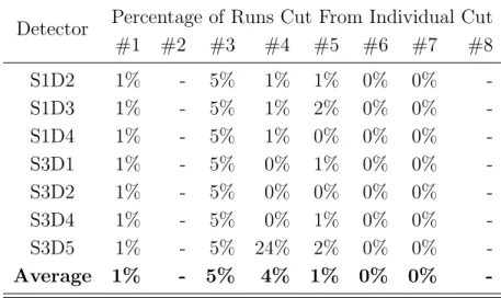
Table 2.2: Percentage of calibration runs cut from each detector after an individual DQ cut is performed. Each cut’s identifying number corresponds to the enumerated cuts described in Section 2.2. Cuts #2 and #8 remove individual events rather than an entire run and are therefore not considered in this table.

Detector Percentage of Runs Cut From Individual Cut

#1 #2 #3 #4 #5 #6 #7 #8

S1D2 1% - 5% 1% 1% 0% 0%

-S1D3 1% - 5% 1% 2% 0% 0%

-S1D4 1% - 5% 1% 0% 0% 0%

-S3D1 1% - 5% 0% 1% 0% 0%

-S3D2 1% - 5% 0% 0% 0% 0%

-S3D4 1% - 5% 0% 1% 0% 0%

-S3D5 1% - 5% 24% 2% 0% 0%

(59)

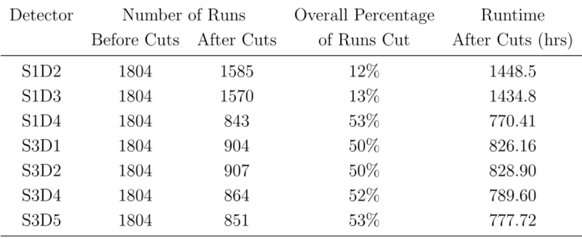
-Table 2.3: Number of background runs before and after DQ cuts. See -Table 2.4 for a breakdown on the percentage of runs that are omitted after each cut.

Detector Number of Runs Overall Percentage Runtime Before Cuts After Cuts of Runs Cut After Cuts (hrs)

S1D2 1804 1585 12% 1448.5

S1D3 1804 1570 13% 1434.8

S1D4 1804 843 53% 770.41

S3D1 1804 904 50% 826.16

S3D2 1804 907 50% 828.90

S3D4 1804 864 52% 789.60

S3D5 1804 851 53% 777.72

Table 2.4: Percentage of background runs cut from each detector after an individual DQ cut is performed. Each cut’s identifying number corresponds to the enumerated cuts described in Section 2.2. Cuts #2 and #8 remove individual events rather than an entire run and are therefore not considered in this table.

Detector Percentage of Runs Cut From Individual Cut

#1 #2 #3 #4 #5 #6 #7 #8

S1D2 1% - 5% 1% 5% 0% 1%

-S1D3 1% - 5% 1% 4% 0% 3%

-S1D4 1% - 5% 1% 47% 0% 5%

-S3D1 1% - 5% 15% - 34% 5%

-S3D2 1% - 5% 15% 1% 34% 2%

-S3D4 1% - 5% 15% 0% 34% 9%

-S3D5 1% - 5% 15% 0% 37% 6%

-Average 1% - 5% 9% 9% 19% 4%